Abstract
With the increasing demand for efficient and accurate numerical simulations of spray combustion in jet engines, the necessity for robust models to enhance the capabilities of spray models has become imperative. Existing approaches often rely on ad hoc determinations or simplifications, resulting in information loss and potentially inaccurate predictions for critical spray characteristics, such as droplet diameters, velocities, and positions, especially under extreme operating conditions or temporal fluctuations. In this study, we introduce a novel approach to modeling multivariate spray characteristics using Gaussian mixture models (GMM). By applying this approach to spray data obtained from numerical simulations of the primary atomization in air-blast atomizers, we demonstrate that GMMs effectively capture the spray characteristics across a wide range of operating conditions. Importantly, our investigation reveals that GMMs can handle complex non-linear dependencies by increasing the number of components, thereby enabling the modeling of more complex spray statistics. This adaptability makes GMMs a versatile tool for accurately representing spray characteristics even under extreme operating conditions. The presented approach holds promise for enhancing the accuracy of spray combustion modeling, offering an improved injection model that accurately captures the underlying droplet distribution. Additionally, GMMs can serve as a foundation for constructing meta models, striking a balance between the efficiency of low-order approaches and the accuracy of high-fidelity simulations.
1. Introduction
The spray combustion process in jet engines consists of complex conjugated physical and chemical processes with multiple time and length scales, making numerical modeling extraordinarily challenging. A computationally effective way to combat these challenges is coupled simulations in which the gaseous phase is modeled in an Eulerian frame of reference and the disperse phase is tracked in a Lagrangian frame of reference. As the physical process is severely influenced by the initial spray characteristics [1], Lagrangian particle tracking (LPT) is also reliant on accurate initial conditions [2,3]. The atomization process responsible for the spray formation is, however, not yet fully understood and difficult to analyze, both experimentally and numerically. Recently, there have been some studies that aim to reduce the computational cost of injector simulations through the use of machine learning techniques and thusly obtained predictions to initialize Euler–Lagrange simulations [4,5,6]. However, these approaches, though promising, are far from mature. Therefore, most Euler–Lagrange spray simulations rely on simplistic injection models that emulate the primary atomization results. In most cases, a droplet diameter distribution based on a characteristic mean diameter is prescribed that is determined either ad hoc through experimental or numerical investigations [7,8,9,10,11], empirical correlations [12,13], or through low-order models [14,15,16,17]. Some authors employ deterministic approaches to determine droplet velocities based on the droplet diameter [9,16], others employ some stochastic methods [18], and in some cases, the droplet velocities are either constant [7,15] or neglected [14]. The spray is usually injected at discrete points distributed evenly around the rotation axis at one or more specified radial distances [7,16]. Some authors employ more sophisticated approaches that incorporate some multivariate stochastic dependencies of the droplet features [19,20]. One approach that should be highlighted is the multivariate injection model by Coblenz et al. [20], which employs vine copulas to accurately reproduce the multivariate dependencies of the individual droplet diameters, velocities, and positions determined through 2D numerical simulation of the primary atomization process [21] and allows for the sampling from these determined statistical distributions. As Coblenz et al. [20] infer, their model also enables the prediction of the spray characteristics for operating conditions that were not part of the preceding numerical study through interpolation of the model parameters.
While these approaches are widely employed and have been demonstrated to be suitable for Euler–Lagrange simulations of spray combustion, they are not without drawbacks. The ad hoc determination or tuning of spray characteristics through either experiment or comprehensive numerical simulation is both exceedingly expensive and difficult. Most more affordable approaches usually necessitate some kind of simplification and thereby inherently exhibit some information loss. The injection model by Coblenz et al. [20] is very appealing due to the possibility of predicting the multivariate dependencies of unknown sprays. However, it is based on parametric ansatz functions that are selected to be suitable for the spray characteristics for their considered geometry of a simplified planar atomizer [13] over their considered operating range. In primary atomization models, the challenges lie in capturing the complex dependencies and interactions of various spray characteristics, such as droplet diameters, velocities, and positions. The parametric ansatz functions used in some models, while suitable for specific geometries and operating ranges, may fail to accurately represent spray behavior under varying conditions, limiting their applicability in critical situations for combustion behavior and the design of atomizers. Of special interest are situations in which the spray characteristics deviate from the optimum, such as extreme operating conditions [22], or through temporal fluctuations induced by thermoacoustic instabilities [23,24], both of which have a significant impact on flame stability and emission characteristics. Another aspect that has to be considered is that a sufficiently sophisticated spray model might feasibly be employed to aid in the design process of atomizers. If a model were able to capture how geometry changes affect spray characteristics, it could possibly be used to markedly shorten design cycles. Similar methods using simplified models are already in use [15]. Beyond primary atomization, a sophisticated spray model may also be used to model other aspects of the spray combustion process, like secondary breakup or evaporation, in the future. This aspiration also necessitates a high level of flexibility that cannot be provided by a model that is inherently dependent on ansatz functions. Therefore, a new approach is required to develop robust models capable of handling complex multivariate dependencies and extending spray modeling capabilities.
To address these limitations, we propose exploring the Gaussian mixture model (GMM) as a new avenue for modeling multivariate spray characteristics. The GMM offers a data-driven technique to model probability distributions through a weighted summation of multiple multivariate normal distributions. Unlike traditional approaches, the GMM does not require ad hoc assumptions about the underlying multivariate dependencies, allowing for a more flexible and accurate representation of spray behavior. By adopting the GMM, we aim to develop a robust spray model that can easily capture intricate dependencies, facilitate straightforward coupling with other models, and seamlessly accommodate additional spray features and mechanisms. Through this approach, we strive to provide a comprehensive and adaptable framework that can significantly enhance the predictive capabilities of spray models and aid in the design process of atomizers, ultimately advancing the understanding and optimization of spray combustion processes in jet engines.
2. Materials and Methods
2.1. Description of the Training Data
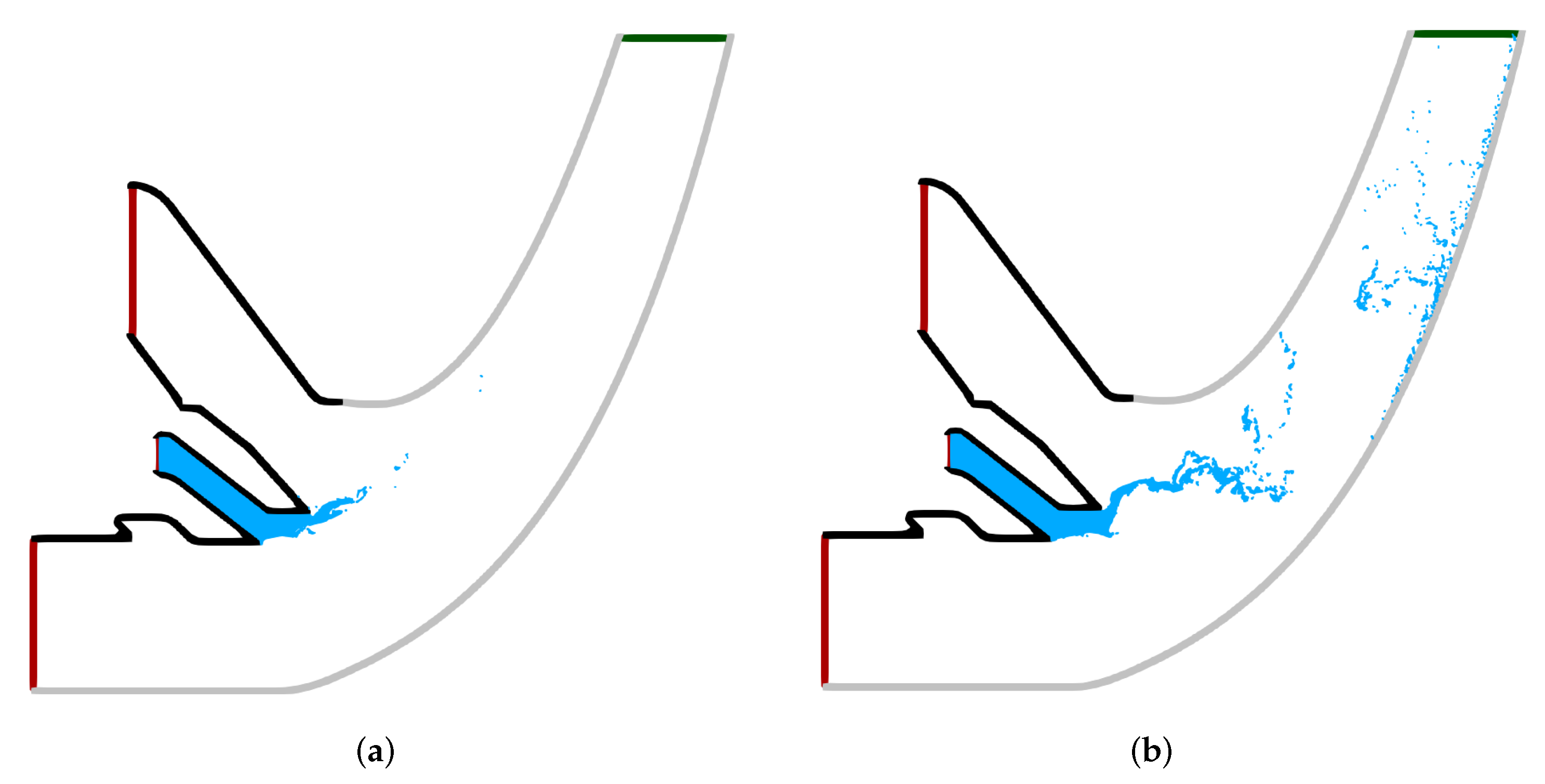
The training data were generated through 2D numerical simulations of the primary atomization process in an air-blast atomizer of a jet engine combustor. These simulations cover four operating points, denoted as , each corresponding to increasing engine load. To perform these simulations, we utilized the smoothed particle hydrodynamics (SPH) method, which was extensively employed in this context. The specific setup for these simulations follows the methodology outlined by Okraschevski et al. [22]. In this setup, the primary atomization process is reduced to two dimensions in a necessary compromise between physical fidelity and computational cost. Despite its simplified two-dimensional approach, the SPH method has demonstrated its capability to accurately capture the spray characteristics [10,11,21,22,25,26]. Figure 1 displays two snapshots from the primary atomization process, one at and the other at , clearly illustrating how the emerging ligament structures and, subsequently, the downstream droplet characteristics are impacted by the change in operating conditions with the decreasing air–fuel ratio. Note that while the gas phase was considered during the simulation, it was excluded from the snapshots to increase visibility of the atomization process and the difference in between the operating points.
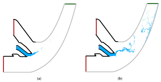
Figure 1.
Impact of operating conditions (OP) on the primary atomization process and the formed droplet size distributions. Inlet and outlet boundary conditions are denoted as red and green, respectively. (a) , (b) .
From these simulations, the spray data are extracted in post-processing at a measurement plane a short distance downstream of the atomization edge. For each droplet, four features are extracted: the equivalent diameter D, the radial distance to the rotation axis r, and axial and radial velocities and . Only liquid fragments consisting of at least four particles or an equivalent diameter of are considered as droplets, and smaller fragments are discarded as numerical artefacts. Each feature is subsequently linearly scaled to the range [0,1] over all operating points. The number of samples N in each data set is shown in Table 1.

Table 1.
Number of droplets N sampled at each operating point .
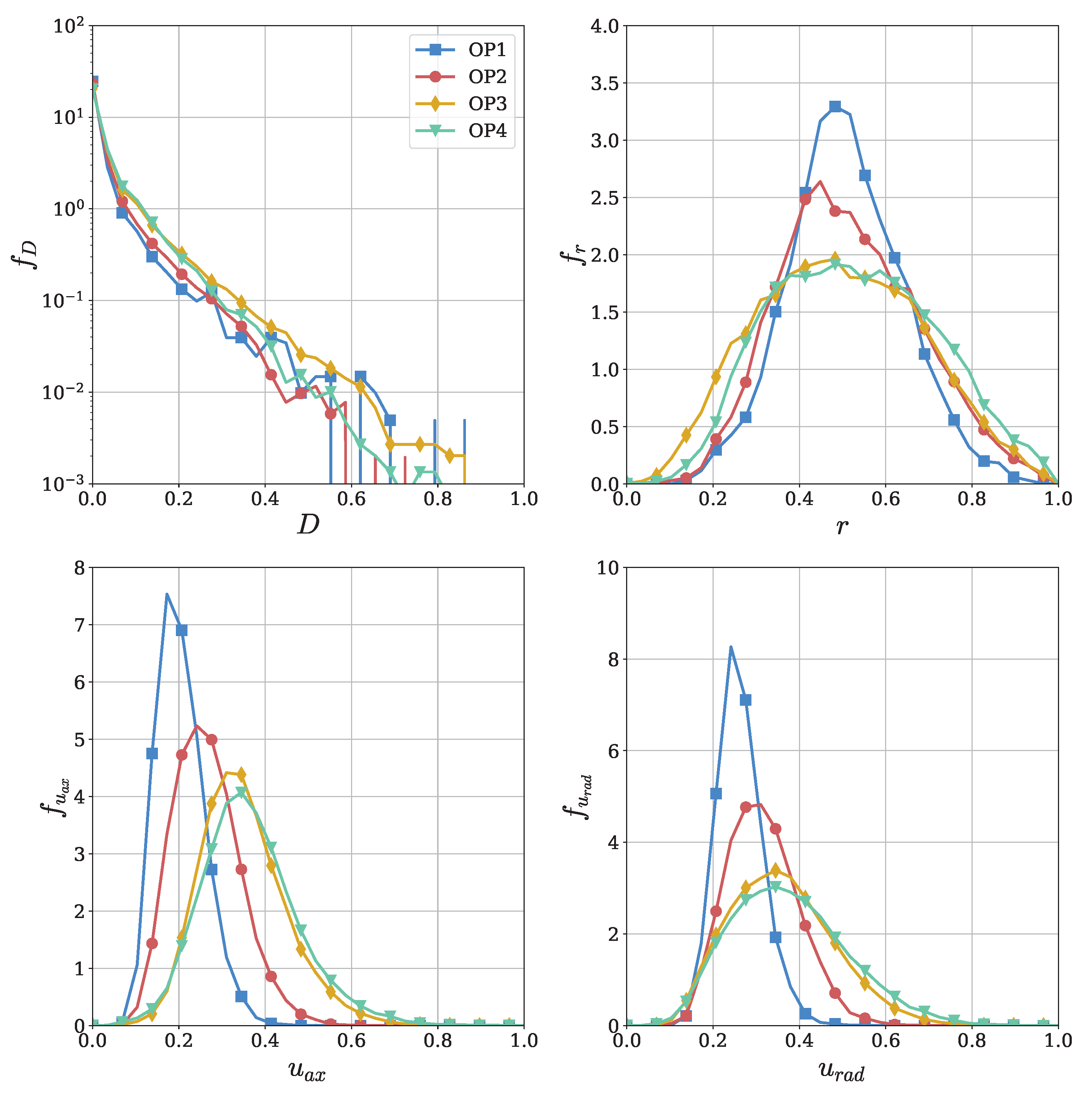
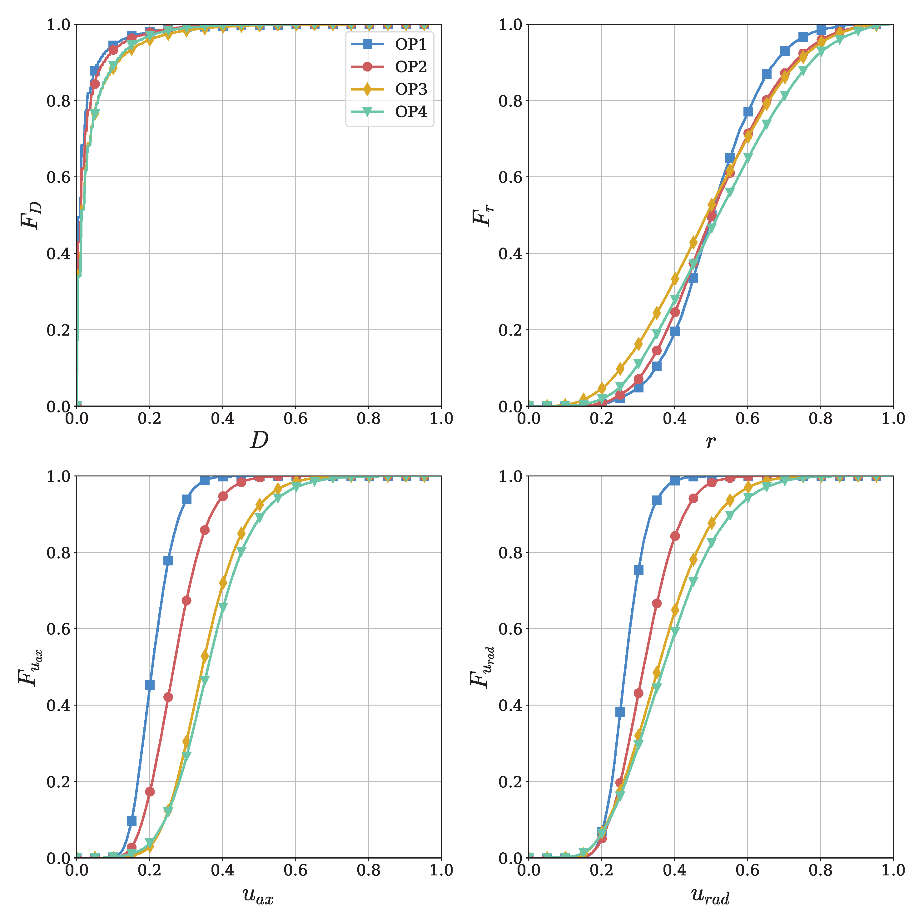
Figure 2 and Figure 3 present the empirical probability density functions (PDFs) f and cumulative distribution functions (CDFs) F, respectively.
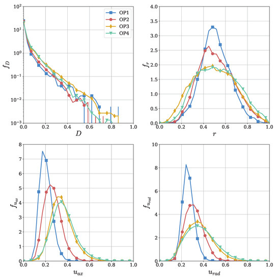
Figure 2.
Univariate PDFs for 4 different ’s with varying load for the equivalent diameter D, the radial distance to the rotation axis r, and axial and radial velocities and .
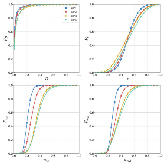
Figure 3.
Univariate CDFs for 4 different s for the equivalent diameter D, the radial distance to the rotation axis r, and axial and radial velocities and .
The probability density is defined as the the number of droplets in the bin k, the bin’s width , and the total number of droplets N as
and the cumulative distribution function is defined as the number of droplets smaller than x divided by the total number of droplets:
The diameter distributions on the top left of both figures exhibit a strong skewness toward the smallest possible values resolved by the SPH simulations. Notably, as the load increases at the operating points, the probability of medium-sized droplets also increases. It is important to note that droplets with a scaled diameter above are extremely rare, leading to CDFs that approach unity beyond . The PDFs of the radial coordinate r resemble Gaussian curves. As the load increases from to , the distributions flatten without a significant shift in the location of their peaks. In the CDFs, this corresponds to a decrease in the slope for higher loads, with a median radial coordinate close to across all operating points. Both axial and radial velocities, and , follow moderately right-skewed bell-shaped PDFs, showing a noticeable trend toward higher values as the load increases. In the CDFs, this corresponds to a combination of a shift toward higher values and decreasing slope.
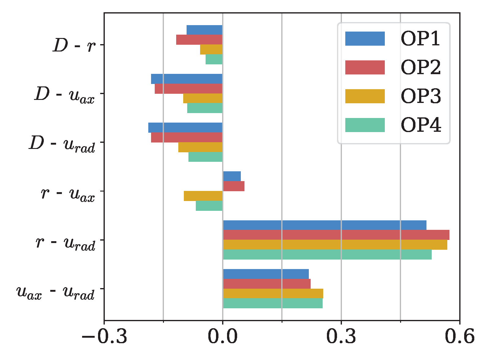
As discussed in the introduction section, the distributions of the droplet features are expected to exhibit statistical interdependence. Herein, the simplest correlations can be quantified and represented using Pearson correlation coefficients, as shown in Figure 4. Notably, there is an inverse correlation between the diameter and other observed features, with the strength of the correlation varying with the operating conditions. Additionally, the axial and radial velocity components are positively correlated, while the strongest correlation exists between radial coordinate and radial velocity.

Figure 4.
Pearson correlation coefficients between the different features for every operating point.
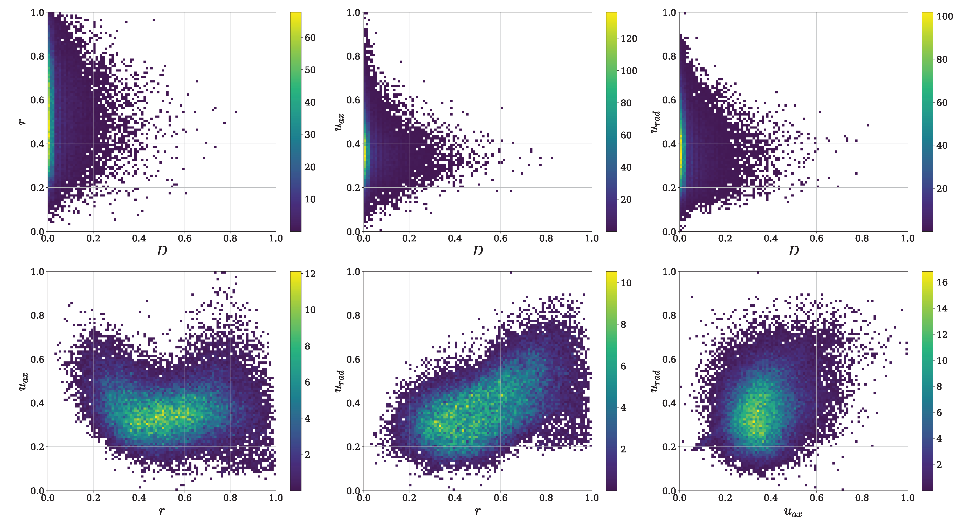
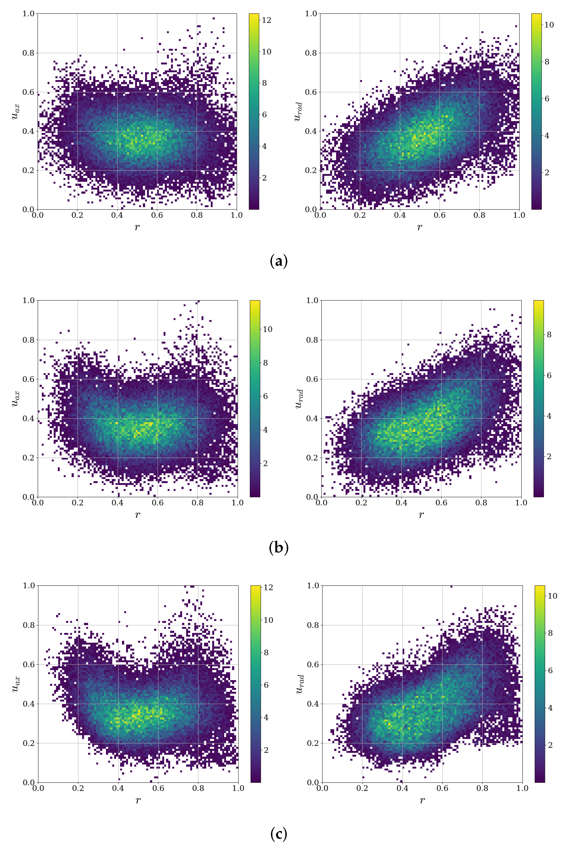
The Pearson correlation coefficients provide valuable information about the basic linear associations between different droplet features. However, it is crucial to acknowledge that these coefficients cannot fully capture the complex multivariate dependencies and nonlinear or non-monotonic relationships that might exist in the data. The limitations of Pearson correlation become evident when considering the bivariate joint PDFs depicted in Figure 5, especially for . These PDFs reveal nonlinear relationships that were not apparent from the Pearson correlation analysis. The PDFs involving the diameter confirm the slight inverse correlation mentioned earlier, while the correlation between radial velocity and radial coordinate aligns with the quantitative findings. However, the joint PDFs uncover an apparent nonlinear relationship between axial velocity and radial coordinate, exhibiting higher axial velocities for small and large droplets, and lower axial velocities for medium-sized droplets.

Figure 5.
Bivariate joint PDFs depicting the nonlinear dependencies in droplet properties at .
These nonlinear and multivariate correlations observed in the droplet statistics emphasize the need for a sophisticated modeling approach. Traditional models may not efficiently capture the intricate interactions and dependencies present in the data. To address this limitation, advanced statistical techniques, such as machine learning algorithms, should be considered. These approaches can effectively handle the complexity of the data, allowing us to capture and utilize the nonlinear and multivariate relationships among droplet features more accurately.
2.2. Gaussian Mixture Model
The Gaussian mixture model (GMM) is a powerful probabilistic model that constitutes the core of our analysis for modeling multivariate spray statistics. It is a flexible model that can capture complex and non-linear relationships between variables, making it suitable for modeling the multivariate spray statistics, where the velocity, position, and diameter features are likely to exhibit intricate dependencies.
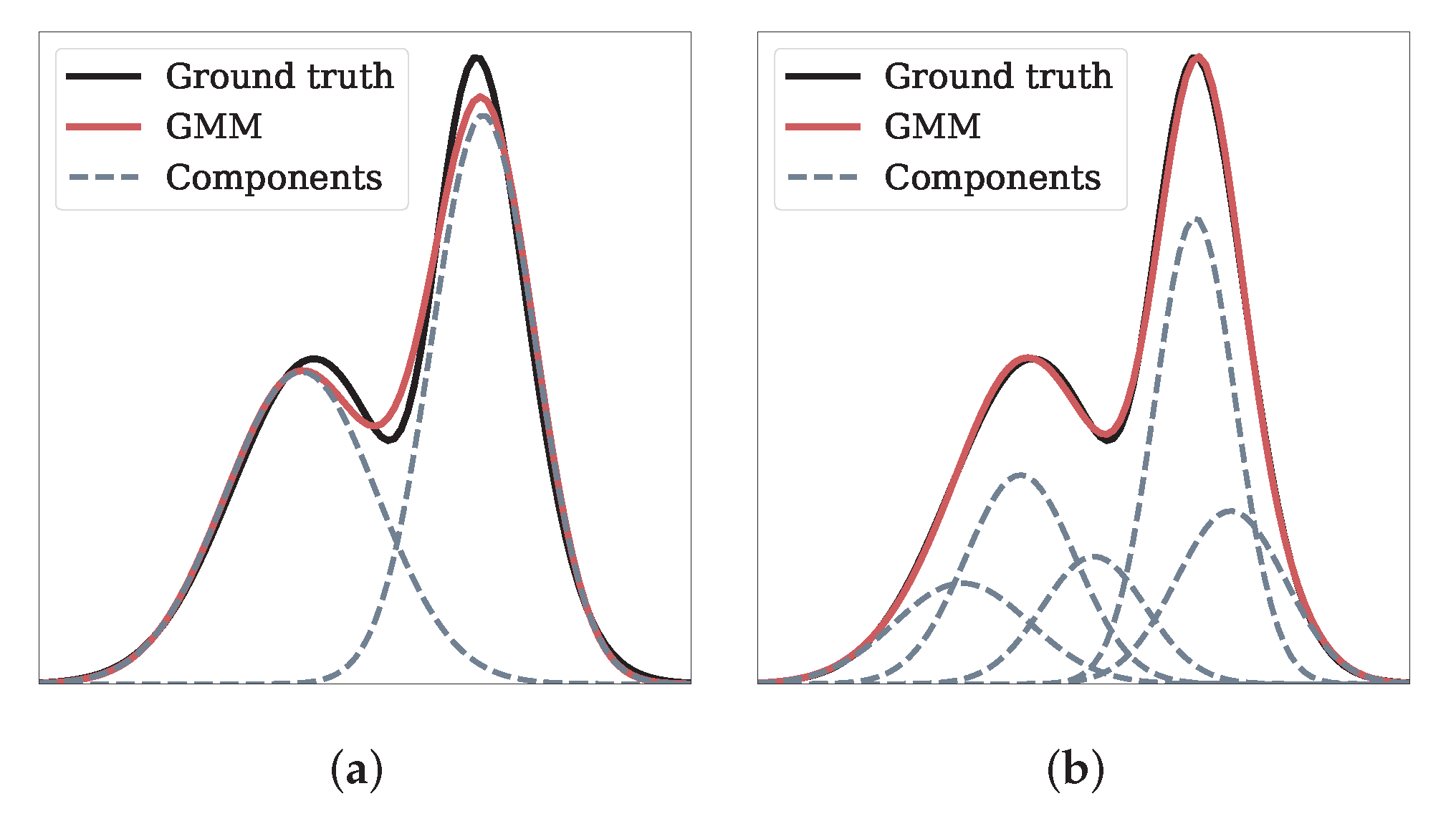
It is based on the assumption that the data are generated from a mixture of multiple Gaussian distributions. Each Gaussian component represents a cluster or mode in the data, and the GMM aims to estimate the parameters of these components to best fit the observed data. The concept is visualized for a bimodal univariate distribution in Figure 6. As evident, if the number of Gaussian components is high enough, the GMM is able to match the ground truth almost exactly.
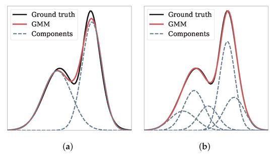
Figure 6.
Visualization of a GMM with n components for a bimodal univariate distribution. (a) ; (b) .
Given a dataset with M data points, the GMM assumes that each data point is generated from one of N Gaussian components with probabilities , where .
The GMM can be mathematically represented as follows:
where
- are the parameters of the GMM,
- is the mean vector of the n-th Gaussian component,
- is the covariance matrix of the n-th Gaussian component, and
- is the weight of the n-th Gaussian component, representing the probability of selecting that component.
Herein, the mean vector represents the central tendency of the data points belonging to that component. It defines the center of a data cluster in the feature space; the covariance matrix characterizes the spread and orientation of the data points within the cluster and captures the interdependencies between different features; and the weight of each component represents the relative contribution of that Gaussian to the overall mixture. In other words, it indicates the likelihood of a data point belonging to a specific cluster.
The goal of GMM training is to find the optimal values for that maximize the likelihood of the observed data. One of the main challenges in learning Gaussian mixture models from unlabeled data is the lack of knowledge about which points belong to which latent component. However, the expectation–maximization (EM) algorithm provides a well-founded statistical approach to address this issue through an iterative process [27]. The EM algorithm consists of two steps: the E-step and the M-step. In the E-step, the algorithm computes the posterior probabilities, or responsibilities, of each data point belonging to the n-th Gaussian component. These probabilities are denoted as and represent the soft assignments of data points to the different components. The E-step can be expressed as:
where is the multivariate Gaussian probability density function of data point with mean and covariance matrix .
In the M-step, the algorithm updates the model parameters based on the responsibilities calculated in the E-step. The updated parameters can be computed as follows:
The EM algorithm iterates between the E-step and M-step until the model parameters converge to a stable solution or a predefined stopping criterion is met. For more details about the EM algorithm for GMM, refer to Chapter 9 of [27].
Model Selection, Initialization, and Evaluation
In an EM algorithm, random components are initially assumed, which can be centered on data points, learned from k-means, or even simply normally distributed around the origin. For each data point, the probability of it being generated by each component of the model is computed. The model’s parameters are then adjusted to maximize the likelihood of the data given these assignments. By repeating this process iteratively, it is ensured that a local optimum is reached by the algorithm. Therefore, during its implementation, two factors need to be decided a priori: (i) the number of Gaussian components, which determines the model complexity, and (ii) the initialization method. In this work, we fit a GMM for each operating point using scikit-learn [28] with full covariance matrices. We increase the number of mixture components up to 30 to explore various model complexities. For each case, the model is trained on the data with 20 random k-means initializations, and the best result is selected. Once the training is completed, the GMM is treated as a generative model, and synthetic droplet distributions of the same size as the training datasets are sampled from each mixture. These synthetic samples are then compared to the training data.
It should be emphasized that evaluating the fit of the Gaussian mixture model is a challenging task, especially when dealing with higher-dimensional dependencies. While univariate and bivariate distributions can be visually analyzed, assessing higher-dimensional dependencies requires a different approach. To tackle this, we employ the Hellinger distance, a measure of similarity between two probability distributions.
The Hellinger distance H is defined for two empirical distributions P and Q with densities p and q, respectively. It is computed using the number of bins k and is given by the equation:
This distance can be computed not only for univariate marginal distributions but also for the multivariate joint distribution. It takes a value of one when there is no overlap between the distributions and a value of zero when they are identical. However, determining the threshold for a good fit is not straightforward due to noise introduced by finite sample sizes in both training and sampled data (the noise in the Hellinger distance depends on the number of bins k and the sample size M). To quantify the distance H to the training data, we utilize another distance , which defines the distance between two synthetic data sets sampled from the same mixture to serve as a “sampling noise”. If the distance H to the training data is comparable to this “sampling noise”, it is reasonable to classify the model as well fitted. We thusly define a loss function L as
Herein, the first term measures the dissimilarities between the four marginal distributions through the distances , while the second term quantifies the multivariate discrepancies between the GMM and the reference data points through the four-dimensional distance . In both terms, we subtract the mean of the corresponding reference distance over all mixtures to account for noise. It should be noted that the magnitude of the distance in high-dimensional 4D data space is expected to be larger; hence, the loss function defined above has an implicit bias to the second term. In other words, it is more descriptive with regard to the multivariate similarities between the GMM predictions and the reference data.
Additionally, we fit and sample from suitable analytical univariate distributions for each droplet feature to establish a benchmark in order to assess the capabilities of GMMs of different complexities to represent univariate distributions. Table 2 shows the assumed analytical distribution functions for each feature: exponentiated Weibull for D, Johnson SB for r, log-normal for , and log-normal for .

Table 2.
Analytical univariate distribution functions for each droplet feature. These distributions are used as a benchmark model to assess the predictive capabilities of the GMM.
3. Results and Discussions
3.1. Assessment of Model Accuracy and Complexity
The first step of the analysis is to determine the appropriate level of complexity, i.e., the number of mixture components needed to accurately represent the spray characteristics of the SPH simulation data. This is achieved by measuring the dissimilarity between CDFs obtained by the GMM model and the ground truth.
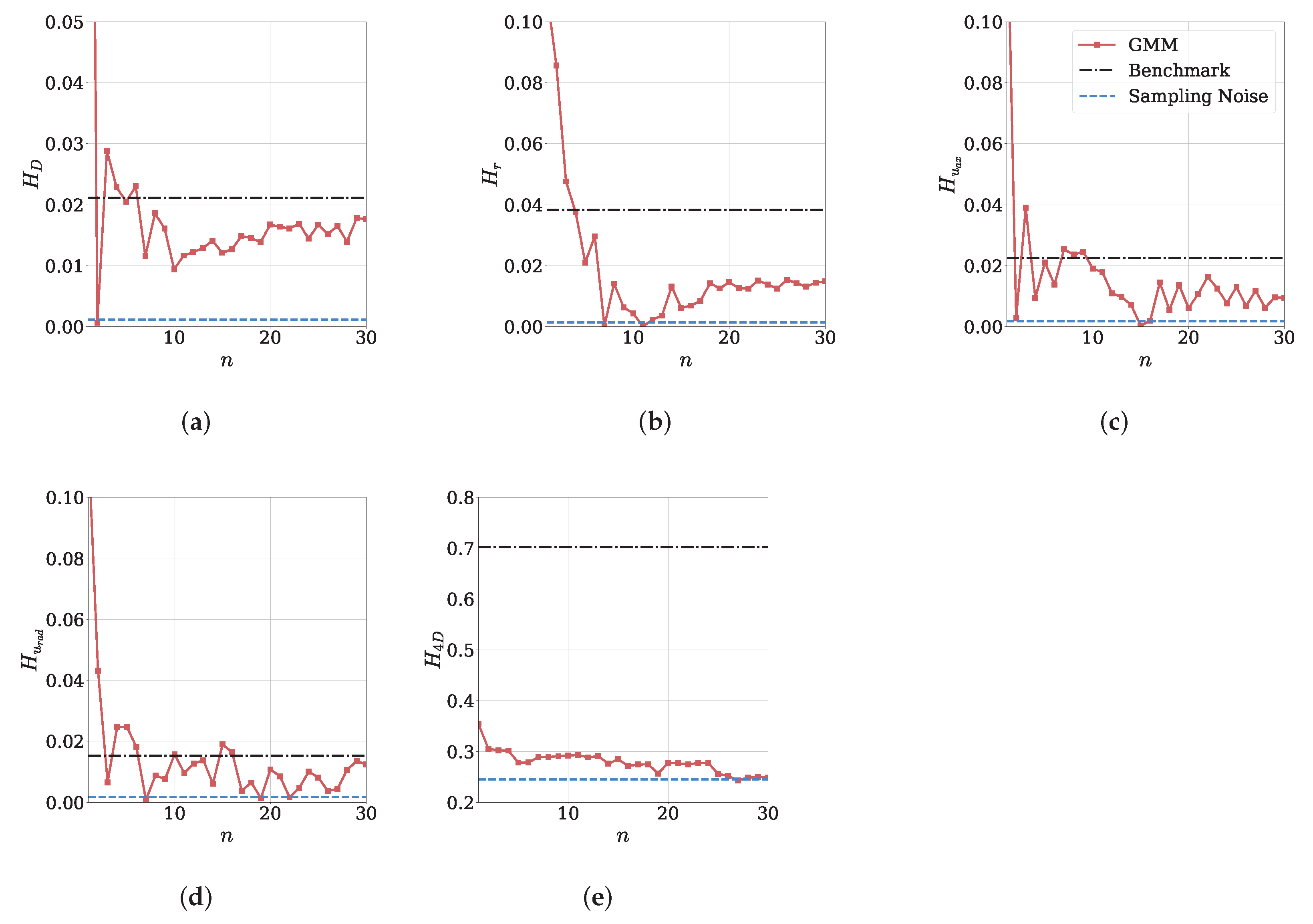
Figure 7 displays the Hellinger distances H for various distributions as a function of the number of Gaussians n for . The computed distances were obtained using 30 bins ( in Equation (6)). Herein, we examine (i) four marginal distributions, diameter D, radial coordinate r, axial velocity , and radial velocity , (ii) as well as the the distances in the four-dimensional data space. It is seen that for all four marginal distributions, the computed distances between the training data and the data sets sampled from the GMM do not converge to the level of uncertainty, which is characterized by the sampling noise in Figure 7. Although an initial downward trend is discernible for all features, the distances for diameter and radial coordinate distributions start to increase again at around . As for the velocity components, their distances appear to fluctuate around a relatively constant value higher than the uncertainty after the initial decrease. Nevertheless, it is worth noting that the magnitude of distances is very small, and lower than the benchmark determined through the distance between the training data and assumed analytical distributions from Table 2. This comparison indicates that while there is no full convergence, the GMM fit leads to a satisfactory accuracy even with few Gaussians for the marginal distributions (Figure 7a–d). Notably and of greater significance, when we compare the Hellinger distances in the 4D space, the change in multivariate distances with an increasing number of Gaussians (i.e., model complexity) does not exhibit the same level of fluctuations. As shown in Figure 7e, the distance decreases more steadily and reaches the level of uncertainty at . This indicates a smoother convergence compared to the individual univariate distributions. Moreover, it becomes apparent that the benchmark assumption of the analytical marginal distributions without any statistical interdependencies is not sufficient to model the training data in the multivariate case, as it fails to account for the correlations between the different features. This comparison clearly underscores the importance of employing multivariate statistical modeling to accurately capture the intricate relationships and dependencies within the spray characteristics.
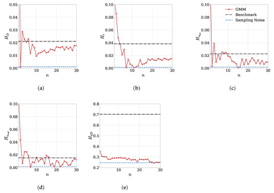
Figure 7.
Evolution of Hellinger distances H as a measure of dissimilarity between the model predictions and the ground truth (GT) with increasing number of Gaussians (n) in GMM for . (a) Diameter D; (b) radial coordinate r; (c) axial velocity ; (d) radial velocity ; (e) 4D droplet data.
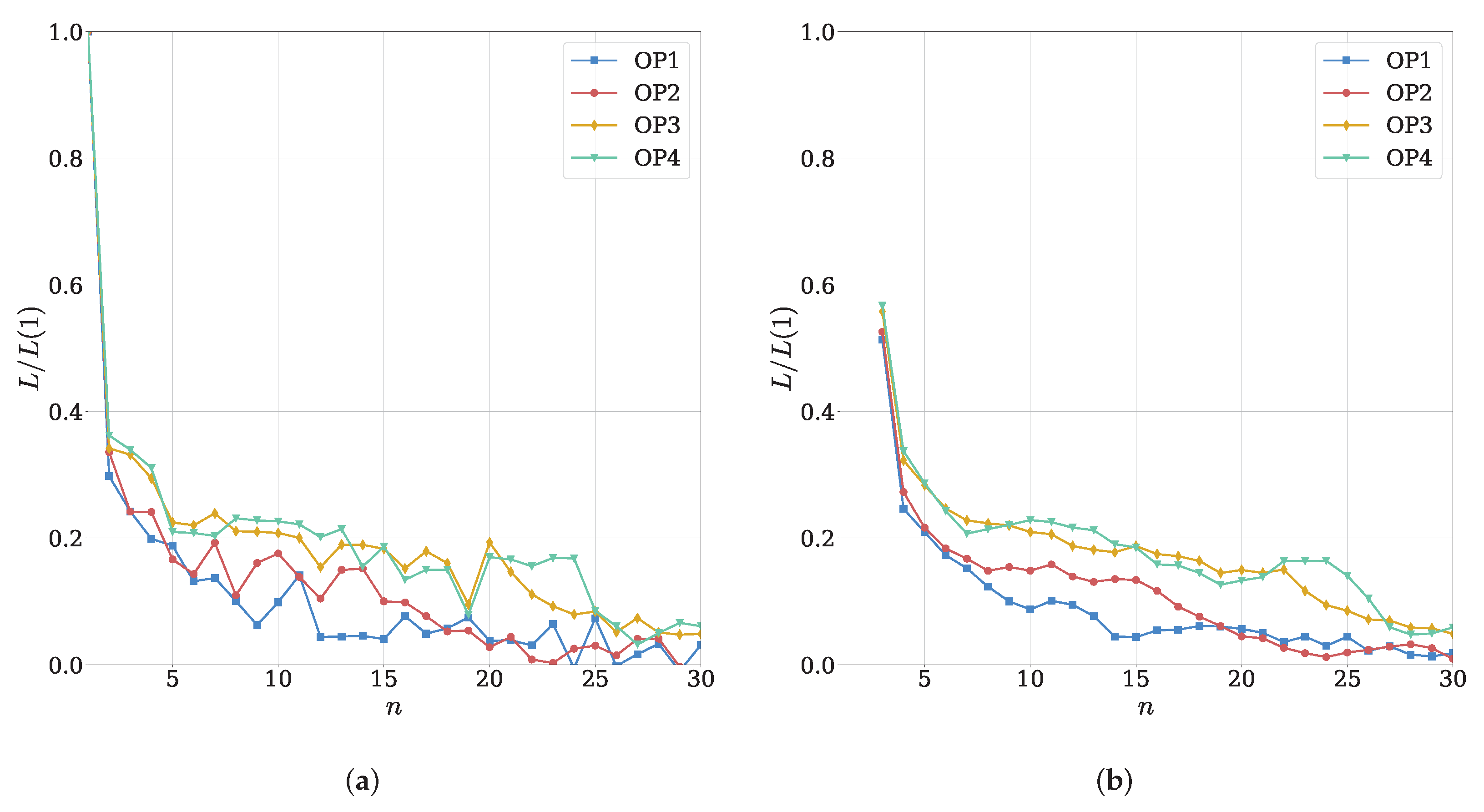
Figure 8 illustrates the evolution of the custom loss function as defined by Equation (7) with an increasing model complexity for all operating points. In this representation, the loss () for a given number of Gaussians (n) is normalized by the loss calculated using only one Gaussian in the GMM, providing a better interpretability as the scaled loss varies between one and zero. Notably, the normalized loss tends to increase as the spray statistics become more complex with an increasing mass load for a given model complexity. Interestingly, the GMM exhibits the ability to yield accurate results with fewer components for simpler cases, such as OP1. Moreover, for each operating point, the rolling mean of the loss functions seems to reach a plateau at a certain number of Gaussians before decreasing again, finally stabilizing at a steady level. This characteristic behavior is evident for all operating points, but convergence occurs later as the load increases.
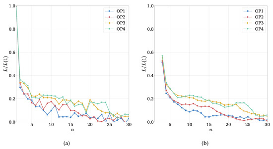
Figure 8.
Normalized loss function using multivariate Hellinger distance. (a) Exact values; (b) rolling mean.
These observations highlight the well-known trade-off between model complexity and accuracy. As the spray characteristics become more intricate, the GMM requires a higher number of components to achieve a satisfactory representation. However, the analysis also reveals that, for certain operating points, a relatively low number of Gaussians may still be sufficient to capture the essential features of the data effectively. This information is crucial for selecting the optimal model configuration that strikes the right balance between complexity and performance in modeling spray characteristics. Another crucial consideration is the risk of overfitting if the model complexity is unnecessarily increased. For example, for OP1, using more than 15 Gaussians may lead to overfitting. Overfitting can result in a model that is too complex and excessively tailored to the training data, which may lead to poor generalization and a subpar performance on new, unseen data.
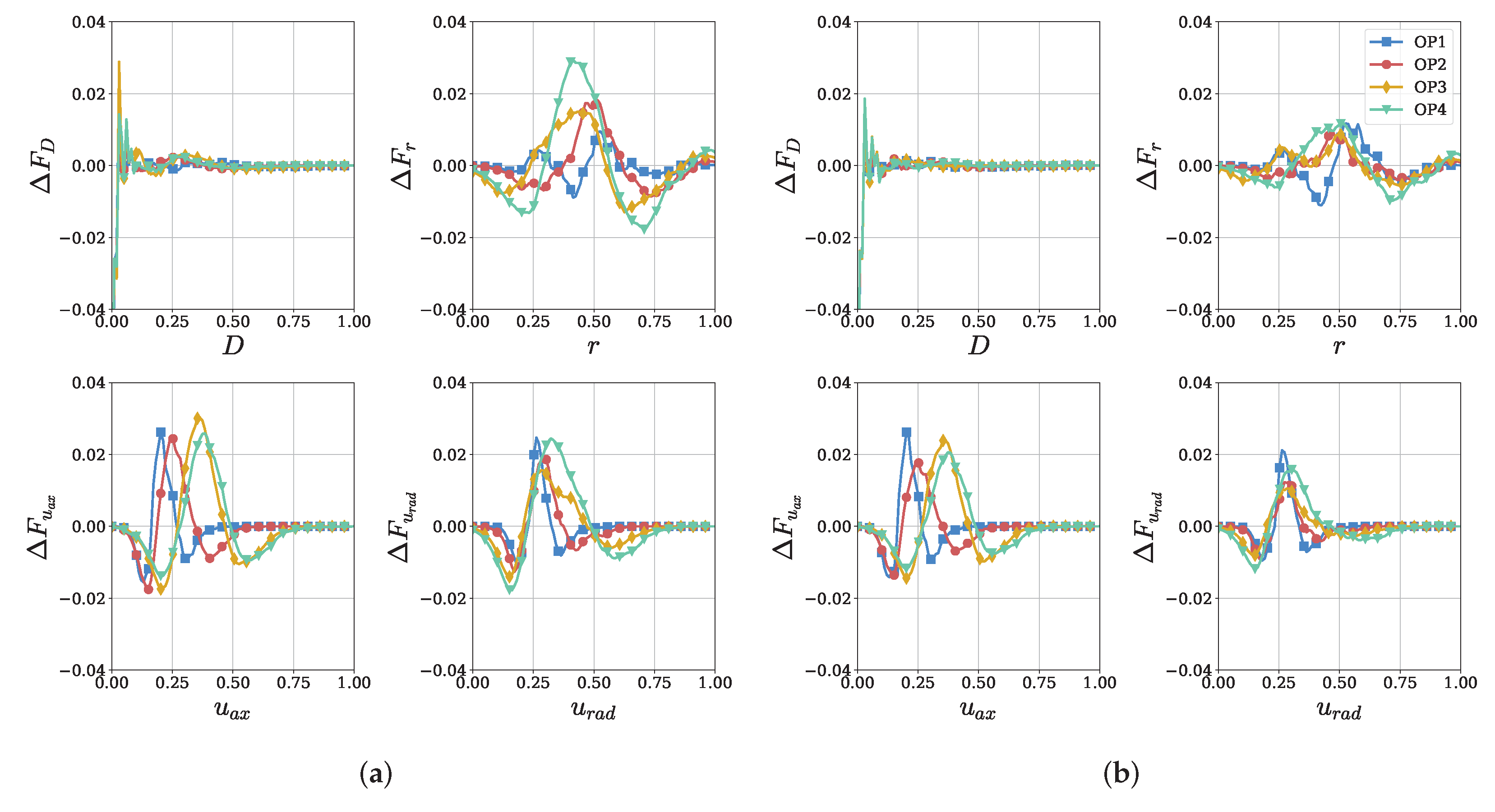
To address these questions, we identify two GMMs for further investigation, one with and the other with . These model complexities correspond to the points where the loss function reaches a steady level for OP1 and OP4. To assess the model error concerning the marginal distributions, we analyze the deviation of the cumulative distribution functions between the training data and the sampled data, denoted as , as shown in Figure 9.
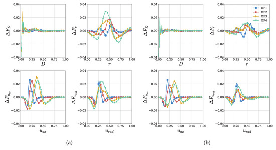
Figure 9.
Deviation of the cumulative distribution functions of the training data and the sampled data with increased model complexity. (a) ; (b) .
For OP1, there is no significant difference between the two mixtures. Both GMMs reproduce the marginal distributions well, with maximum errors ranging between and . This suggests that increasing the number of components beyond the optimum complexity only results in splitting the noise-related Gaussian components and does not significantly affect the model’s overall accuracy. In other words, an increased model complexity does not lead to a significant generalization penalty. However, for OP4, the GMM with proves to be insufficient in modeling the distribution of the radial coordinate, as the error is more than twice as large compared to OP1. By increasing the model complexity to , this error is notably reduced to a similar level as observed for the other operating points. While the improvement from to is not as drastic for the other features, it is still significant.
These findings emphasize the significance of selecting an appropriate model complexity that can accurately capture the underlying distribution of the data for each operating point. Furthermore, it is essential to note that the GMM is not an over-parameterized model like artificial-neural-network-based generative models such as variational autoencoders (VAEs) or generative adversarial networks (GANs). Therefore, the risk of overfitting is considerably lower and less likely to be a concern in a GMM-based approach.
3.2. Conservation of Feature Correlations
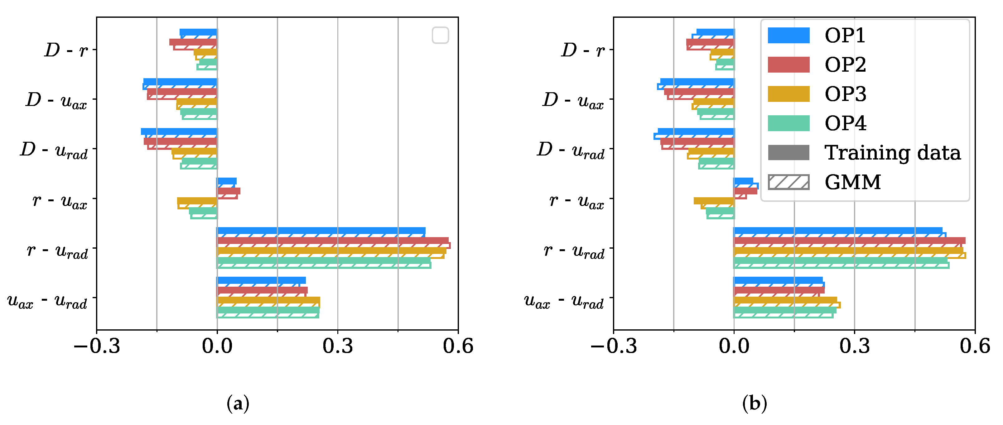
One crucial expectation from generative models is their ability to preserve the underlying correlations observed in the training set (i.e., source domain) when generating synthetic spray statistics. To evaluate the GMM’s performance in this regard, we quantify the feature correlations using Pearson correlation coefficients, as depicted in Figure 10.
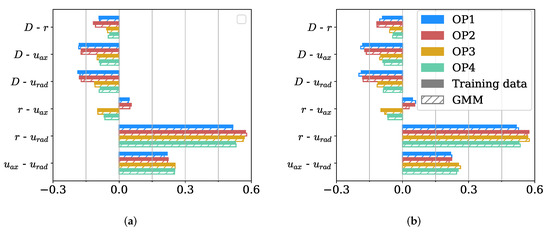
Figure 10.
Comparison of the Pearson correlation coefficients of the training data and sampled data. Solid bars denote the ground truth, while dashed bars give the GMM predictions. Colors denote the operating points. (a) ; (b) .
Remarkably, even at a moderate model complexity, i.e., , the GMM effectively captures these correlations. Both mixtures closely reproduce the correlation coefficients of the training data, demonstrating the model’s ability to preserve the linear relationships between the features even with a low number of Gaussians. However, it is important to note that the Pearson correlation coefficients cannot fully capture non-linear relationships, as discussed in Section 2.1. To gain further insights, a visual evaluation of the bivariate joint PDFs becomes necessary. A selection of these joint PDFs is presented in Figure 11.
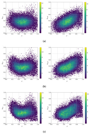
Figure 11.
Bivariate joint PDFs of radial coordinate and axial velocity (left) and radial coordinate and radial velocity (right) of the GMM and the training data for . (a) ; (b) ; (c) training data.
The linear correlation between radial coordinate and radial velocity on the right hand side of the figure is well resolved by both mixtures. Nevertheless, the mixture with struggles to capture the characteristic shape of the bivariate PDF between radial coordinate and axial velocity, which is present in the training data. This observation suggests that a higher number of components is necessary to model probability densities of such complex shapes. However, with , the GMM successfully reproduces the sampled data, visually aligning with the distribution of the training data.
4. Conclusions
In summary, the GMM proves to be adept at capturing linear correlations between features, even at moderate model complexities. However, for more intricate non-linear relationships, a higher number of components is required for an accurate representation. The visual evaluation of the bivariate joint PDFs provides valuable insights into the model’s ability to preserve complex correlations in the spray data, making it a powerful tool for the accurate statistical modeling of spray characteristics across different operating conditions. We are confident that the approach presented in this study can be readily extended to incorporate additional droplet features, such as shape and temperature, without incurring unreasonable complexities. By increasing the number of components, the Gaussian mixture models (GMMs) can effectively accommodate these new features, enhancing the comprehensiveness of spray simulations. The findings of this study demonstrate that GMMs offer a promising and easily implementable injection model for improving spray simulations in the future. With their ability to accurately capture spray characteristics at any arbitrary state, GMMs hold the potential to serve as valuable tools for constructing meta models. These meta models could bridge the gap between the efficiency of common low-order approaches and the accuracy of high-fidelity simulations in numerical spray modeling. Overall, the versatility and efficiency of GMMs make them an attractive choice for advancing spray engineering and optimizing combustion processes. By incorporating a wide range of droplet features and developing meta models, GMMs offer a promising path toward achieving improved spray simulations and enhancing our understanding of complex spray dynamics in jet engine combustors.
Author Contributions
Conceptualization, C.A., M.O., S.H. and M.W.; methodology, C.A. and M.W.; software, C.A., M.O. and M.W.; formal analysis, C.A., M.O., M.W. and R.K.; writing—original draft preparation, C.A. and M.W.; writing—review and editing, M.O., S.H., R.K. and H.-J.B.; visualization, M.O. and M.W.; supervision, C.A., R.K. and H.-J.B.; project administration, R.K. and H.-J.B.; funding acquisition, R.K. and H.-J.B. All authors have read and agreed to the published version of the manuscript.
Funding
This research received no external funding.
Data Availability Statement
Not applicable.
Acknowledgments
The authors acknowledge support by the state of Baden-Württemberg through bwHPC. We acknowledge support by the KIT-Publication Fund of the Karlsruhe Institute of Technology.
Conflicts of Interest
The authors declare no conflict of interest.
Abbreviations
The following abbreviations are used in this manuscript:
| CDF | Cumulative distribution function |
| GMM | Gaussian mixture model |
| GT | Ground truth |
| Probability density function | |
| SPH | Smoothed particle hydrodynamics |
References
- Kuo, K.K.; Acharya, R. Fundamentals of Turbulent and Multiphase Combustion; Wiley Online Library, Wiley: Hoboken, NJ, USA, 2012. [Google Scholar] [CrossRef]
- Bürkle, N.; Holz, S.; Bärow, E.; Koch, R.; Bauer, H.J. Effect of Droplet Starting Conditions on the Spray Dispersion Resulting From a Swirl Cup Injector. In Proceedings of the Volume 2C: Turbomachinery—Design Methods and CFD Modeling for Turbomachinery; Ducts, Noise, and Component Interactions; American Society of Mechanical Engineers: New York, NY, USA, 2021. [Google Scholar] [CrossRef]
- Puggelli, S.; Paccati, S.; Bertini, D.; Mazzei, L.; Giusti, A.; Andreini, A. Multi-coupled numerical simulations of the DLR Generic Single Sector Combustor. Combust. Sci. Technol. 2018, 190, 1409–1425. [Google Scholar] [CrossRef]
- Milan, P.J.; Torelli, R.; Lusch, B.; Magnotti, G.M. Data-Driven Model Reduction of Multiphase Flow In a Single-Hole Automotive Injector. At. Sprays 2020, 30, 401–429. [Google Scholar] [CrossRef]
- Mondal, S.; Torelli, R.; Lusch, B.; Milan, P.J.; Magnotti, G.M. Accelerating the Generation of Static Coupling Injection Maps Using a Data-Driven Emulator. SAE Int. J. Adv. Curr. Pract. Mobil. 2021, 3, 1408–1424. [Google Scholar] [CrossRef]
- Milan, P.J.; Mondal, S.; Torelli, R.; Lusch, B.; Maulik, R.; Magnotti, G.M. Data-Driven Modeling of Large-Eddy Simulations for Fuel Injector Design. In Proceedings of the AIAA Scitech 2021 Forum, Reston, VA, USA, 11–15 January 2021. [Google Scholar] [CrossRef]
- Jones, W.P.; Marquis, A.J.; Vogiatzaki, K. Large-eddy simulation of spray combustion in a gas turbine combustor. Combust. Flame 2014, 161, 222–239. [Google Scholar] [CrossRef]
- Keller, J.; Gebretsadik, M.; Habisreuther, P.; Turrini, F.; Zarzalis, N.; Trimis, D. Numerical and experimental investigation on droplet dynamics and dispersion of a jet engine injector. Int. J. Multiph. Flow 2015, 75, 144–162. [Google Scholar] [CrossRef]
- Gallot-Lavallée, S.; Jones, W.P.; Marquis, A.J. Large Eddy Simulation of an ethanol spray flame under MILD combustion with the stochastic fields method. Proc. Combust. Inst. 2017, 36, 2577–2584. [Google Scholar] [CrossRef]
- Chaussonnet, G.; Joshi, S.; Wachter, S.; Koch, R.; Jakobs, T.; Kolb, T.; Bauer, H.J. Air-Assisted Atomization at Constant Mass and Momentum Flow Rate: Investigation into the Ambient Pressure Influence with the Smoothed Particle Hydrodynamics Method. J. Eng. Gas Turbines Power 2020, 142, 031019. [Google Scholar] [CrossRef]
- Ates, C.; Karwan, F.; Okraschevski, M.; Koch, R.; Bauer, H.J. Conditional Generative Adversarial Networks for modelling fuel sprays. Energy AI 2023, 12, 100216. [Google Scholar] [CrossRef]
- Lefebvre, A. Atomization and Sprays; CRC Press: Boca Raton, FL, USA, 1988. [Google Scholar] [CrossRef]
- Gepperth, S.; Koch, R.; Bauer, H.J. Analysis and Comparison of Primary Droplet Characteristics in the Near Field of a Prefilming Airblast Atomizer. In Proceedings of the Volume 1A: Combustion, Fuels and Emissions; American Society of Mechanical Engineers: New York, NY, USA, 2013. [Google Scholar] [CrossRef]
- Chaussonnet, G.; Vermorel, O.; Riber, E.; Cuenot, B. A new phenomenological model to predict drop size distribution in Large-Eddy Simulations of airblast atomizers. Int. J. Multiph. Flow 2016, 80, 29–42. [Google Scholar] [CrossRef]
- Comer, A.L.; Kipouros, T.; Stewart Cant, R. Multi-objective Numerical Investigation of a Generic Airblast Injector Design. J. Eng. Gas Turbines Power 2016, 138, 091501. [Google Scholar] [CrossRef]
- Sanjosé, M.; Senoner, J.M.; Jaegle, F.; Cuenot, B.; Moreau, S.; Poinsot, T. Fuel injection model for Euler–Euler and Euler–Lagrange large-eddy simulations of an evaporating spray inside an aeronautical combustor. Int. J. Multiph. Flow 2011, 37, 514–529. [Google Scholar] [CrossRef]
- Inamura, T.; Shirota, M.; Tsushima, M.; Kato, M.; Hamajima, S.; Sato, A. Spray characteristics of prefilming type of airblast atomizer. In Proceedings of the ICLASS, 12th Triennial International Annual Conference on Liquid Atomization and Spray Systems, Heidelberg, Germany, 2–6 September 2012. [Google Scholar]
- Hoffmann, S.; Holz, S.; Koch, R.; Bauer, H.J. Euler–Lagrangian simulation of the fuel spray of a planar prefilming airblast atomizer. CEAS Aeronaut. J. 2021, 12, 245–259. [Google Scholar] [CrossRef]
- Apte, S.V.; Mahesh, K.; Moin, P. Large-eddy simulation of evaporating spray in a coaxial combustor. Proc. Combust. Inst. 2009, 32, 2247–2256. [Google Scholar] [CrossRef]
- Coblenz, M.; Holz, S.; Bauer, H.J.; Grothe, O.; Koch, R. Modelling Fuel Injector Spray Characteristics in Jet Engines by Using Vine Copulas. J. R. Stat. Soc. Ser. Appl. Stat. 2020, 69, 863–886. [Google Scholar] [CrossRef]
- Holz, S.; Braun, S.; Chaussonnet, G.; Koch, R.; Bauer, H.J. Close Nozzle Spray Characteristics of a Prefilming Airblast Atomizer. Energies 2019, 12, 2835. [Google Scholar] [CrossRef]
- Okraschevski, M.; Mesquita, L.C.C.; Koch, R.; Mastorakos, E.; Bauer, H.J. A Numerical Study of Aero Engine Sub-idle Operation: From a Realistic Representation of Spray Injection to Detailed Chemistry LES-CMC. Flow Turbul. Combust. 2023, 111, 493–530. [Google Scholar] [CrossRef]
- Chaussonnet, G.; Müller, A.; Holz, S.; Koch, R.; Bauer, H.J. Time-Response of Recent Prefilming Airblast Atomization Models in an Oscillating Air Flow Field. J. Eng. Gas Turbines Power 2017, 139, 121501. [Google Scholar] [CrossRef]
- Lo Schiavo, E.; Laera, D.; Riber, E.; Gicquel, L.; Poinsot, T. Effects of liquid fuel/wall interaction on thermoacoustic instabilities in swirling spray flames. Combust. Flame 2020, 219, 86–101. [Google Scholar] [CrossRef]
- Braun, S.; Wieth, L.; Holz, S.; Dauch, T.F.; Keller, M.C.; Chaussonnet, G.; Gepperth, S.; Koch, R.; Bauer, H.J. Numerical prediction of air-assisted primary atomization using Smoothed Particle Hydrodynamics. Int. J. Multiph. Flow 2019, 114, 303–315. [Google Scholar] [CrossRef]
- Dauch, T.F.; Chaussonnet, G.; Keller, M.C.; Okraschevski, M.; Ates, C.; Koch, R.; Bauer, H.J. 3D Predictions of the Primary Breakup of Fuel in Spray Nozzles for Aero Engines. In High Performance Computing in Science and Engineering ’20; Nagel, W.E., Kröner, D.H., Resch, M.M., Eds.; Springer International Publishing: Cham, Switzerland, 2021; pp. 419–433. [Google Scholar] [CrossRef]
- Bishop, C.M. Pattern Recognition and Machine Learning; Information Science and Statistics; Springer: New York, NY, USA, 2006. [Google Scholar]
- Pedregosa, F.; Varoquaux, G.; Gramfort, A.; Michel, V.; Thirion, B.; Grisel, O.; Blondel, M.; Prettenhofer, P.; Weiss, R.; Dubourg, V.; et al. Scikit-learn: Machine Learning in Python. J. Mach. Learn. Res. 2011, 12, 2825–2830. [Google Scholar]
Disclaimer/Publisher’s Note: The statements, opinions and data contained in all publications are solely those of the individual author(s) and contributor(s) and not of MDPI and/or the editor(s). MDPI and/or the editor(s) disclaim responsibility for any injury to people or property resulting from any ideas, methods, instructions or products referred to in the content. |
© 2023 by the authors. Licensee MDPI, Basel, Switzerland. This article is an open access article distributed under the terms and conditions of the Creative Commons Attribution (CC BY) license (https://creativecommons.org/licenses/by/4.0/).

