Investigation of Flow Fields Emanating from Two Parallel Inlet Valves Using LES, PIV, and POD

Abstract

Understanding cycle-to-cycle variations (CCV) is of practical importance for the combustion of fossil and renewable fuels, as increasingly stringent emission regulations require reductions in the negative effects of such variations. The subject of this study is the flow around inlet valves, since oscillations of such inlet flows affect the flow structure in the cylinder and are thus one of the causes of CCV. To this end, a parametric analysis of the influences of the mass flow rate and valve lift of two parallel engine intake valves on the flow structures is performed. This follows on from an earlier similar study where the flow around a single intake valve was investigated. To analyse the flow behaviour and, in particular, the interactions of the flow leaving these two valves, an optical test rig for 2D particle image velocimetry (PIV) and a large eddy simulation (LES) are used. Proper orthogonal decomposition (POD), together with a quadruple decomposition and the Reynolds stress transport equations, are used to study the turbulence phenomena. The PIV and LES results are in good agreement with each other. The detailed LES analysis of the flow structures shows that, for small valve lifts, the flow separates along the whole perimeter of the intake valve, and for larger valve lifts, the flow escapes only to one side. This is, for combustion engines with the tumble concept, the stage at which the tumble movement develops. Moreover, the flow structures are strongly influenced by the valve lift, while they are unaffected by the variation in the mass flow. The turbulent kinetic energy in the flow field increases quadratically with a decreasing valve lift and increasing mass flow. The large, high-energetic flow structures are particularly dominant near the jet, and the small, low-energetic structures are homogeneously distributed within the flow field. The specific Reynolds stress transport equation shows the limitations of two-dimensionality and large timesteps in the PIV results and the limitations of the LES model.

1. Introduction

1.1. Motivation

Although electric vehicles are becoming increasingly popular due to the growing awareness of climate change and the impact of combustion emissions, the internal combustion engine will continue to play a vital role, especially in transportation and power generation [1]. This is not least because of the high energy density of the corresponding fuels from both fossil and renewable sources [2]. However, in order to reduce the negative impact of internal combustion engine emissions on the environment, the corresponding emission regulations are becoming increasingly stringent, which poses major challenges for the further development of such engines. To effectively address this problem, a multi-faceted approach from different perspectives is required, taking into account all factors that influence engine emissions.

Reducing fuel consumption together with harmful emissions is a primary objective in the development of internal combustion engines. Among the various strategies investigated, such as external exhaust gas recirculation (EGR), stratified combustion, lean combustion, and homogeneous charge compression ignition, thermal efficiency offers the highest potential for improvement [3]. However, cycle-to-cycle fluctuations present a significant challenge to optimising combustion. These fluctuations can result in increased engine emissions, reduced efficiencies, and abnormal combustion phenomena, as previously studied in the works of Young [4,5], Ozdor [6,7], and Ball [8]. Therefore, understanding and mitigating cycle-to-cycle variations (CCV) hold great promise for the development of future high-efficiency internal combustion engines. One factor that influences these variations is the oscillation of the inflow jet, which has a significant impact on the flow structure inside the cylinder. This is especially crucial for the velocity field surrounding the spark plug during ignition, as well as other processes such as mixture formation and combustion.

The complex problem of cycle-to-cycle fluctuations in internal combustion engines has been studied for many years [9,10,11]. Since the combustion process in an engine involves multiple parallel and sequential mechanisms, the underlying causes are interconnected and influence one another. A possible cause–effect chain of CCV includes factors such as the inlet flow [12,13,14], injection strategy, and mixture formation, as well as the thermofluidic state at the spark plug during ignition [15]. Among these factors, the inlet inflow, which determines the level of turbulence, is considered the most significant as it impacts subsequent processes, for example, mixture formation and combustion [6,16]. Therefore, the airflow around the engine valves plays a vital role in the combustion and mixing processes and has been extensively investigated [12,17,18,19,20,21,22,23,24,25,26,27,28].

For controlling air motion, combustion engines utilise various components, such as intake ports [12,18,19,20,29], fuel injection systems [12,13,30], the piston shape [31,32,33], tumble/swirl flaps [27], intake valves [34,35], and the valve lift [36,37,38]. Two main types of flow can be observed in the cylinder: Tumble and swirl, with rotation axes perpendicular to and around the cylinder axis, respectively. Typically, spark ignition engines prioritise tumble motion [19,39,40], while compression ignition engines employ intake channels engineered to enhance swirl [29,39,40].

Research on CCV has revealed that tumble motion experiences significant fluctuations, particularly during the closing of the inlet valve, leading to variations in turbulence during combustion [9,10,13,25,36,41,42]. Tumble flow is commonly found in modern high-efficiency gasoline engines. Previous findings have shown that combustion engines with strong tumble generation tend to have higher turbulence levels compared to those with swirl flows; however, they are also more susceptible to CCV in the flow field within the combustion chamber, particularly up to the point of ignition [11]. Recent numerical investigations have also highlighted that secondary flows caused by inflow jet oscillations can superimpose on the main charge flow, resulting in variations in the flow velocities around the spark plug that, in turn, influence flame kernel growth [43]. Fluctuations in the flow field near the spark plug at the time of ignition significantly contribute to CCV, as reported by Hasse [15].

Traditional non-intrusive measurement techniques such as laser Doppler anemometry (LDA), particle image velocimetry (PIV), and magnetic resonance velocimetry (MRV) have been widely used for studying in-cylinder flow in combustion engines [27,44,45,46,47,48,49,50,51]. High-speed PIV is a suitable method for measuring time-resolved in-cylinder flow fields and capturing CCV as well as large-scale fluctuations [52,53]. This technique can provide insights into intake inflow jet oscillations, including detachment at the valve seat and secondary flow structures. To further analyse and process the data obtained from PIV, the proper orthogonal decomposition (POD) filtering approach is commonly applied [19,25,48,54,55,56,57]. POD allows for the separation of measured flow fields into dominant, coherent, and turbulent small-scale structures. The POD results can serve as reference validation data for numerical models of CCV in combustion engines. In addition, the POD approach has been used for the identification of the spatial structure and temporal evolution of a flow field within an engine obtained by means of 3D high-speed PIV [55].

Experimental studies on in-cylinder flow in combustion engines often focus on one or two specific planes, such as the symmetry plane, tumble plane, parallel planes, cross-tumble plane (orthogonal to the symmetry plane), or horizontal planes [7,54,58,59,60,61]. While there are various optically accessible engine test rigs that enable the application of different optical techniques, occasionally, there is a need for ad-hoc test rigs to replicate specific air flows or to provide better accessibility [19,33,34,35,40,62,63,64,65,66,67]. However, a drawback of such engine test benches is frequently lower flexibility regarding the operating parameters, such as the intake pressure and temperature, as well as the limitation to stationary flows with constant valve lifts. This should be taken into consideration when interpreting experimental results and their applicability to real-world engine conditions.

The use of 3D computational fluid dynamics (CFD) simulations provides a cost-effective way to investigate complex phenomena, such as CCV, in detail, in comparison to experiments. The Reynolds-averaged Navier–Stokes (RANS) simulation approach is commonly used in engine development. In particular, the RANS k-ε turbulence model performs well for predicting the flow field in engine applications [9]. Nevertheless, RANS approaches are not suitable for studying cyclic fluctuations, due to their averaging nature. Instead, the use of detached eddy simulation (DES) or Large Eddy Simulation (LES) methods is more common in this context [53]. The LES method resolves the large structures directly, and the small turbulent structures, which are computationally expensive to resolve, are modelled [21]. The validation of LES with measurements in terms of CCV has shown good agreement. [10,52,68]. However, LES places higher requirements on the spatial and temporal resolutions of the flow field, and multiple cycles need to be computed to replicate CCV. All this together leads to higher computing times. DES provides a good compromise between LES and RANS, where the RANS method is utilised for near-wall areas or regions with coarse grid resolution, whereas LES is used for separated flows further away from walls or free shear layers. DES has been used successfully for studying CCV in some studies [69]. LES has emerged as a solution to the challenges faced by direct numerical simulations (DNS), which are computationally much more demanding.

1.2. State-of-the-Art

Recent studies have concentrated on PIV investigations to analyse the influences of various engine parameters on the in-cylinder flow. A recent study by Hoffmann et al. [70] presented a thorough literature review on the different types of in-cylinder airflow in optical engines and experimental test rigs. It also presented an experimental and numerical study of the air flow through a single valve with simplified engine geometry. Therefore, this section focuses on dual valves and real engine geometry.

Be it computational simulations or experimental investigations, the use of simplified geometry instead of real engine geometry can cause significant differences in terms of accuracy and the level of detail captured. Although a simplified geometry may be easier to build and can be useful for initial concept evaluations or in cases where computational resources are limited, it may not accurately represent the complex and intricate geometry of a real engine. Real engine geometry includes features and intricate details of the intake systems, such as valve seats and port shapes. These details can significantly affect the flow characteristics, turbulence, and swirl within the engine. Real engine geometry may also impact the operational conditions used in simulations. The complex geometry of intake and exhaust ports, for example, can affect the flow rates, pressure profiles, and turbulence levels at the inlet and outlet of the engine. Simplified geometry may not accurately capture these operational conditions, which can affect the accuracy of the simulations.

Many studies have used simplified geometry models, such as flow benches or scaled models, to investigate the intake flow and mixing characteristics of internal combustion engines. However, recent research has focused on using realistic engine geometry to gain a more accurate analysis of intake flow. Previous studies presented by Keskinen and Antila studied the intake flow characteristics of a single-cylinder engine via CFD using realistic engine geometry [71,72,73]. The intake port of a diesel engine was studied via CFD simulations to enhance the swirl and improve the flow characteristics. The results were validated using a steady-flow, dual-valve test rig with real engine geometry [74]. An experimental study by El-Adawy et al. characterised the inlet port flow in a test rig with real engine geometry using PIV and POD. To do this, a real four-valve pent-roof gasoline direct injection (GDI) cylinder head was mounted on top of the optical accesses [75]. Another study ran a simulation with four different piston bowl geometries and observed that the piston bowl played a predominant role in the air pattern inside the cylinder [76]. A numerical study investigated the incompressible flow in the intake pipe of an engine at a constant valve position with real-engine-like geometry [77].

In an engine with a single intake valve, there is only one valve that controls the flow of the air–fuel mixture into the combustion chamber. This is typically used in older or smaller engines and is simpler in terms of design and operation. It opens and closes to let the air–fuel mixture into the combustion chamber during the intake stroke and then closes during the compression stroke, whereas in an engine with dual intake valves, there are two valves that control the flow of the air–fuel mixture into the combustion chamber, and these valves work together to optimise the engine’s performance. The advantages of dual intake valves over a single intake valve include improved airflow into the combustion chamber, increased power and torque output, and better fuel efficiency. However, it is noteworthy that the design and performance of an engine are influenced by various factors, and the number of intake valves is just one of them.

The shape, size, number, and synchronisation of the intake valves play crucial roles in the generation of swirl and tumble during the admission stroke, which is highly dependent on the specific air intake and valve configuration [78]. Various other factors can also impact the flow in the cylinder and consequently affect the swirl and tumble. The impact of swirl and tumble on combustion within the cylinder has been widely studied, and its effect on the shape of the flame front has been directly observed in experiments [13,79]. Previous research focused on the influence of intake valves on the generation of swirl and tumble by using different geometries [80]. Two recent studies demonstrated that the use of asynchronous intake valves resulted in the creation of a vortex, based on the concept of tumble, which influenced the movement of air and enhanced turbulent kinetic energy during the mixing process. As a result, this led to a reduction in the coefficient of variation of the indicated mean effective pressure (COV-IMEP) [81,82]. Another study investigated the effect of valve timing on fuel consumption and concluded that brake-specific fuel consumption (BSFC) was reduced and knocking at high loads was mitigated [83]. These findings suggest that the design and configuration of intake valves play vital roles in the overall performance of the engine, including its fuel efficiency and emissions.

1.3. Objectives and Content

The main objective of this investigation is to understand the effects of valve lift variation and different mass flows in a dual-valve setup with real-engine geometry using a low-speed PIV technique. The aim is to expand and complement the findings presented in a previous investigation [70]. Even though the boundary conditions may not be representative of a real combustion engine with moving internals and transient flow, the results obtained from the new setup will provide insights into the flow characteristics as well as generate reference validation data under steady-state conditions. These data can then be used to analyse various conditions in more realistic engine simulations.

2. Fundamentals

The following section presents the fundamentals, starting with the characteristics of turbulent flows, followed by the Reynolds stress transport equation. After that, the proper orthogonal decomposition (POD) filtering approach is introduced together with the quadruple decomposition of the POD modes in order to spilt them into the mean value as well as the dominant, coherent, and turbulent structures.

2.1. Turbulent Flows

Within turbulent flows, there are eddies within a wide range of length scales, leading to an effective exchange of mass, momentum, and heat. According to the energy cascade, the largest, inviscid, and most energetic eddies have anisotropic structures and are affected by the mean flow direction. To fulfil momentum conservation, those vortices are stretched, and the kinetic energy is transferred from larger to smaller eddies. As a result, the rotational rate of the eddies increases, and their radii decrease. The smallest, viscous eddies, with the lowest amount of energy, are isotropic, and their energy is dissipated into thermal energy, which leads to increased energy loss in turbulent flows [84].

The variances and covariances of the velocity fluctuation components lead to additional (shear and normal) stress components. Those variances and covariances can be found, multiplied by the negative value of the density $\rho$, in the Reynolds stress tensor ${\stackrel{⃡}{\tau }}_{RS}$ in Equation (1), describing the momentum transfer owing to turbulent eddies.

$${\stackrel{⃡}{\tau }}_{RS}=\left(\begin{array}{ccc}-\overline{\rho u_x^{\prime 2}}& -\overline{\rho u_x^{\prime }{u}_y{}^{\prime }}& -\overline{\rho u_x^{\prime }{u}_z{}^{\prime }}\\ -\overline{\rho u_x^{\prime }{u}_y{}^{\prime }}& -\overline{\rho u_y^{\prime 2}}& -\overline{\rho u_y^{\prime }{u}_z{}^{\prime }}\\ -\overline{\rho u_x^{\prime }{u}_z{}^{\prime }}& -\overline{\rho u_y^{\prime }{u}_z{}^{\prime }}& -\overline{\rho u_z^{\prime 2}}\end{array}\right)$$

(1)

2.2. Reynolds Stress Transport Equation

The specific Reynolds stress transport equation was derived for the incompressible case with a constant kinematic viscosity $\nu$ and is shown in Equation (2). There are six independent components of the specific Reynolds stresses, and there is one equation for each of them. The various terms in Equation (2) can be interpreted as shown in Equation (3), where the different terms are described below.

$$\begin{array}{cc}\frac{\partial \overline{u_i^{\prime }\cdot u_j{}^{\prime }}}{\partial t}+\nabla \cdot \hfill & \left(\overline{u_i^{\prime }\cdot u_j{}^{\prime }}\cdot \overline{\overrightarrow{u}}\right)\hfill \\ & =\nabla \cdot \left(\nu \nabla \overline{u_i^{\prime }\cdot u_j{}^{\prime }}\right)-\nabla \cdot \left(\overline{u_i^{\prime }\cdot u_j^{\prime }\cdot \overrightarrow{u}{}^{\prime }}\right)-\frac{1}{\rho }\left(\frac{\partial \overline{p^{\prime }\cdot u_i^{\prime }}}{\partial x_j}+\frac{\partial \overline{p^{\prime }\cdot u_j^{\prime }}}{\partial x_i}\right)\hfill \\ & -\left(\left(\overline{u_i^{\prime }\cdot \overrightarrow{u}{}^{\prime }}\cdot \nabla \right){\overline{u}}_j+\left(\overline{u_j^{\prime }\cdot \overrightarrow{u}{}^{\prime }}\cdot \nabla \right){\overline{u}}_i\right)+\frac{1}{\rho }\overline{p^{\prime }\left(\frac{\partial \overline{u_i^{\prime }}}{\partial x_j}+\frac{\partial \overline{u_j^{\prime }}}{\partial x_i}\right)}\hfill \\ & -2\nu \overline{\left(\nabla u_i^{\prime }\right)\cdot \left(\nabla u_j^{\prime }\right)}\hfill \end{array}$$

(2)

$$R_{ij}+C_{ij}=D_{MT,ij}+D_{TT,ij}+D_{PVF,ij}+P_{ij}+{\Pi }_{ij}+E_{ij}$$

(3)

• $R_{ij}$: The rate of change in specific Reynolds stress in the control volume;
• $C_{ij}$: The convective flux over the surfaces of the control volume;
• $D_{MT,ij}$: The diffusive flux owing to molecular transport;
• $D_{TT,ij}$: The diffusive flux owing to turbulent transport;
• $D_{PVF,ij}$: The diffusive flux owing to pressure/velocity fluctuations;
• $P_{ij}$: The production term of the specific Reynolds stress;
• ${\mathsf{\Pi }}_{ij}$: The pressure–strain correlation;
• $E_{ij}$: The dissipation rate of the specific Reynolds stress.

2.3. Proper Orthogonal Decomposition (POD)

POD is often used to evaluate turbulent flows from particle image velocimetry (PIV) measurements in the field of fluid dynamics. The main idea is to decompose random vector fields into a set of deterministic functions, where each captures an amount of the total fluctuating turbulent kinetic energy of the flow situation [85].

2.3.1. The Direct POD Method

The goal of the POD method is the decomposition of the random vector fields $u^{\prime }(x,t)$ into deterministic spatial functions ${\mathsf{\Phi }}_k\left(x\right)$ (spatial modes) and their corresponding random time coefficients $a_k\left(t\right)$, according to Equation (4) [85].

$$u^{\prime }\left(x,t\right)=\sum _{k=1}^{1000}{a}_k\left(t\right){\mathsf{\Phi }}_k\left(x\right)$$

(4)

It begins with the snapshot matrix $U$, which is presented in Equation (5), which contains all of the velocity fluctuations. Each of the matrix components $u_{ij}^{\prime }$ corresponds to the fluctuation velocity at point $j$ ($1\le j\le n$) for time $i$ ($1\le i\le m$). The fluctuation velocity is calculated from the PIV data by the difference compared to the time-averaged velocity. $U$ is an $m\times n$ matrix with $m=1000$ instant times and $n={23}^{\prime }474$ data points (total number of velocity vectors) for both velocity components in the $x$- and $y$-directions [85].

$$U=\left(\begin{array}{cccc}{u^{\prime }}_{11}& {u^{\prime }}_{12}& \cdots & {u^{\prime }}_{1n}\\ {u^{\prime }}_{21}& {u^{\prime }}_{22}& \cdots & {u^{\prime }}_{2n}\\ ⋮& ⋮& \ddots & ⋮\\ {u^{\prime }}_{m1}& {u^{\prime }}_{m2}& \cdots & {u^{\prime }}_{mn}\end{array}\right)$$

(5)

After that, the covariance matrix $C$, which is a symmetric $n\times n$ matrix, is computed. The diagonal elements of the matrix $C$ shown in Equation (6) correspond to the variances, and the off-diagonal elements correspond to the covariances [85].

$$C=\frac{1}{m-1}{U}^{T}U=\frac{1}{m-1}\left(\begin{array}{cccc}{\displaystyle \sum _{i=1}^m}{u^{\prime }}_{i1}^2& {\displaystyle \sum _{i=1}^m}{u^{\prime }}_{i1}\cdot {u^{\prime }}_{i2}& \cdots & {\displaystyle \sum _{i=1}^m}{u^{\prime }}_{i1}\cdot {u^{\prime }}_{in}\\ {\displaystyle \sum _{i=1}^m}{u^{\prime }}_{i2}\cdot {u^{\prime }}_{i1}& {\displaystyle \sum _{i=1}^m}{u^{\prime }}_{i2}^2& \cdots & {\displaystyle \sum _{i=1}^m}{u^{\prime }}_{i2}\cdot {u^{\prime }}_{in}\\ ⋮& ⋮& \ddots & ⋮\\ {\displaystyle \sum _{i=1}^m}{u^{\prime }}_{in}\cdot {u^{\prime }}_{i1}& {\displaystyle \sum _{i=1}^m}{u^{\prime }}_{in}\cdot {u^{\prime }}_{i2}& \cdots & {\displaystyle \sum _{i=1}^m}{u^{\prime }}_{in}^2\end{array}\right)=\left(\begin{array}{cccc}{c}_{11}& c_{12}& \cdots & c_{1n}\\ c_{21}& c_{22}& \cdots & c_{2n}\\ ⋮& ⋮& \ddots & ⋮\\ c_{n1}& c_{n2}& \cdots & c_{nn}\end{array}\right)$$

(6)

Finally, the eigenvalue problem $C{\mathsf{\Phi }}_k=\lambda {\mathsf{\Phi }}_k$ is solved. The eigenvectors ${\mathsf{\Phi }}_k$ are called POD modes. They are orthonormal and describe the correlations of the fluctuations as well as how they move with each other. The time coefficients can be calculated from $A=U{\mathsf{\Phi }}_k$. The eigenvalues $\lambda$ are a measure of the amount of energy in each mode. Finally, the modes ${\mathsf{\Phi }}_k$ and eigenvalues $\lambda$ are ranked in descending order of $\lambda$, with the first few modes containing the largest amounts of energy. Equation (4) shows how the original data within the snapshot matrix $U$ can be reconstructed by summing up over all time coefficients $a_k\left(t\right)$ multiplied by the corresponding spatial mode ${\mathsf{\Phi }}_k\left(x\right)$ [85].

2.3.2. The Snapshot POD Method

The snapshot POD method is similar to the direct POD method. In the snapshot POD method, time and space are interchanged compared to the direct one. The deterministic temporal modes ${\mathsf{\Phi }}_k\left(t\right)$ and the random spatial coefficients $a_k\left(x\right)$ are computed instead of the spatial modes ${\mathsf{\Phi }}_k\left(x\right)$ and the time coefficients $a_k\left(t\right)$. Because the last eigenvalues of the direct method are zero anyway, and the number of instant times is smaller than the number of data points $m<n$, the snapshot method is computationally less expensive. The snapshot matrix $U_s$ ($n\times m$) can be computed from $U_s=U^T$. The eigenvalues ${\lambda }_s=\lambda$ are equal to the ones computed by the direct method. The modes and coefficients of the snapshot method are proportional to those of the direct method. Because of this, the spatial coefficients ${\mathsf{\Phi }}_{ks}$ can be normalised to obtain the spatial modes ${\mathsf{\Phi }}_k$ [85].

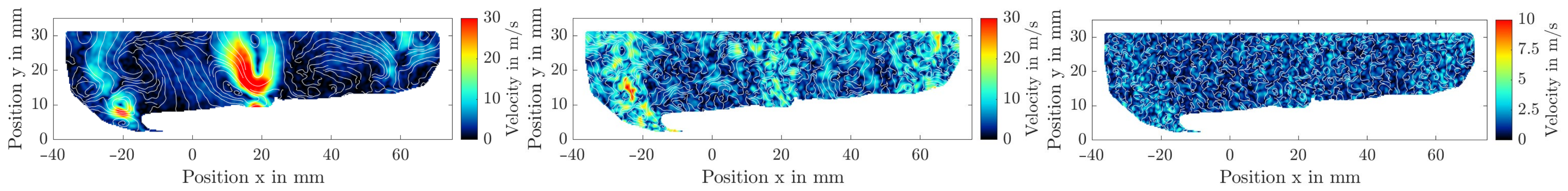
2.4. POD Quadruple Decomposition

Druault et al. 2005 [86], Roudnitzky et al. 2006 [87], Vu et al. 2012 [25], Rulli et al. 2021 [88], and Wu et al. 2022 [89] proposed the POD quadruple decomposition to split the turbulent structures into dominant, coherent, and turbulent structures by means of POD. The velocity $u(x,t)$ can be split into a mean value $\overline{u}\left(x\right)$ and the fluctuation $u^{\prime }(x,t)$, where $u^{\prime }(x,t)$ can further be decomposed into the dominant, coherent, and turbulent structures, according to Equation (7).

$$u\left(x,t\right)=\overline{u}\left(x\right)+u_{\mathrm{dominant}}^{\prime }\left(x,t\right)+u_{\mathrm{coherent}}^{\prime }\left(x,t\right)+u_{\mathrm{turbulent}}^{\prime }(x,t)$$

(7)

The relevance index shown in Equation (8) proposed by Wu et al. 2022 [89] is used to compare the vector fields of the $x$- and the $y$-velocity components of two neighbouring POD modes regarding their similarity. To identify the cut-off mode between the dominant and the coherent structures, a target value between 0.9 and 1 [89], namely, 0.9935 [70], was chosen.

$$R_i=\frac{\overline{\overrightarrow{a_i{\mathsf{\Phi }}_i}·\overrightarrow{a_{i+1}{\mathsf{\Phi }}_{i+1}}}}{\overline{\overrightarrow{a_i{\mathsf{\Phi }}_i}}\cdot \overline{\overrightarrow{a_{i+1}{\mathsf{\Phi }}_{i+1}}}}$$

(8)

According to Roudnitzky et al. 2006 [87], the skewness and the flatness (kurtosis) coefficients, $S_i$ and $T_i$, defined in the Equations (9) and (10) are suitable for finding the cut-off number between the coherent and turbulent structures. Homogeneous isotropic turbulent flow is assumed to have Gaussian properties. For turbulent structures, a skewness $S_i$ of zero is expected, since $S_i$ defines the third standardised central moment of a distribution. The flatness $T_i$ is a measure of the tailedness of a probability distribution and characterises the shape of this distribution, where for a normal distribution, a value of three results [88].

$$S_i=\frac{\overline{\overrightarrow{{\left(a_i{\mathsf{\Phi }}_i\right)}^3}}}{{\overline{\overrightarrow{{\left(a_i{\mathsf{\Phi }}_i\right)}^2}}}^{3/2 }}$$

(9)

$$T_i=\frac{\overline{\overrightarrow{{\left(a_i{\mathsf{\Phi }}_i\right)}^4}}}{{\overline{\overrightarrow{{\left(a_i{\mathsf{\Phi }}_i\right)}^2}}}^{2 }}$$

(10)

3. Methodology

According to Hoffmann et al. [70], a novel test rig was designed and commissioned. In this study, the test bench was modified to examine how the flow characteristics around two parallel intake valves are affected by variations in the mass flow rate and valve lift. In the following chapter, the test rig as well as the optical technique and the image processing are described. Besides this, the large eddy simulation (LES) model, which is described in the next chapter, is validated using the reference data set obtained with particle image velocimetry (PIV).

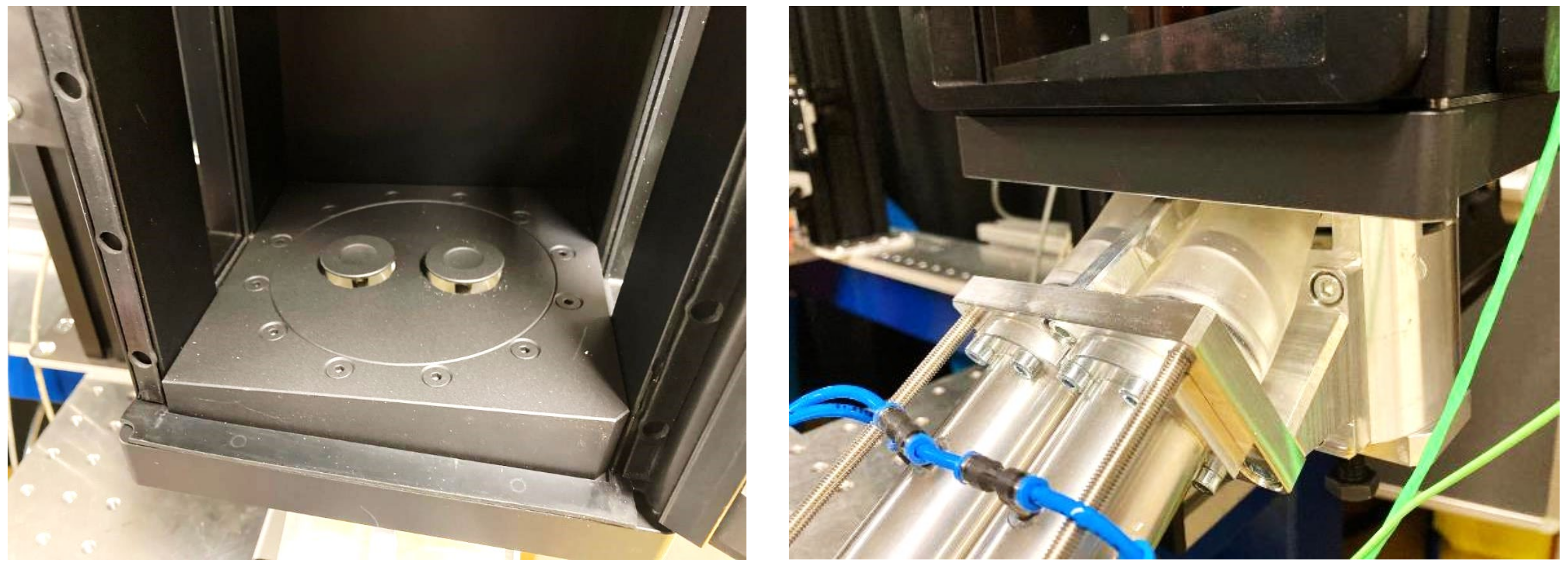
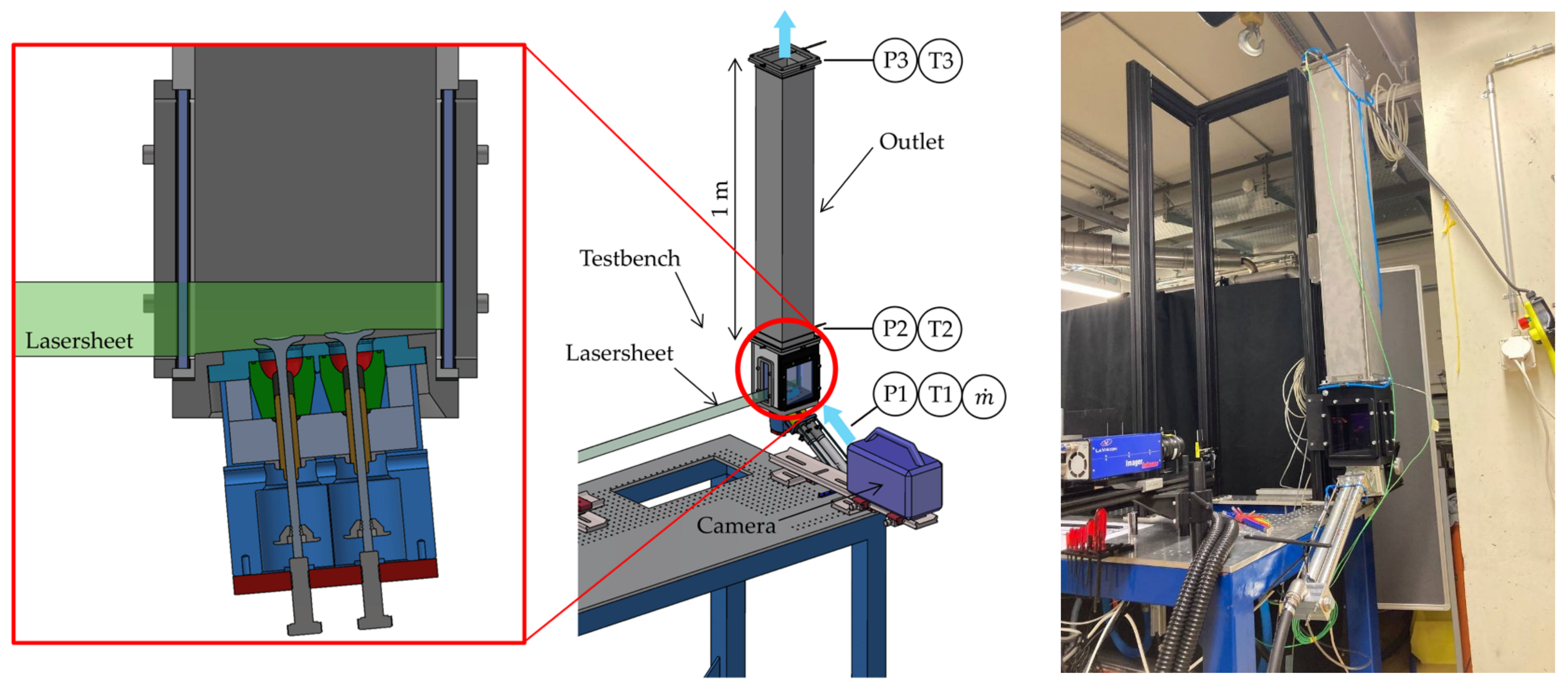
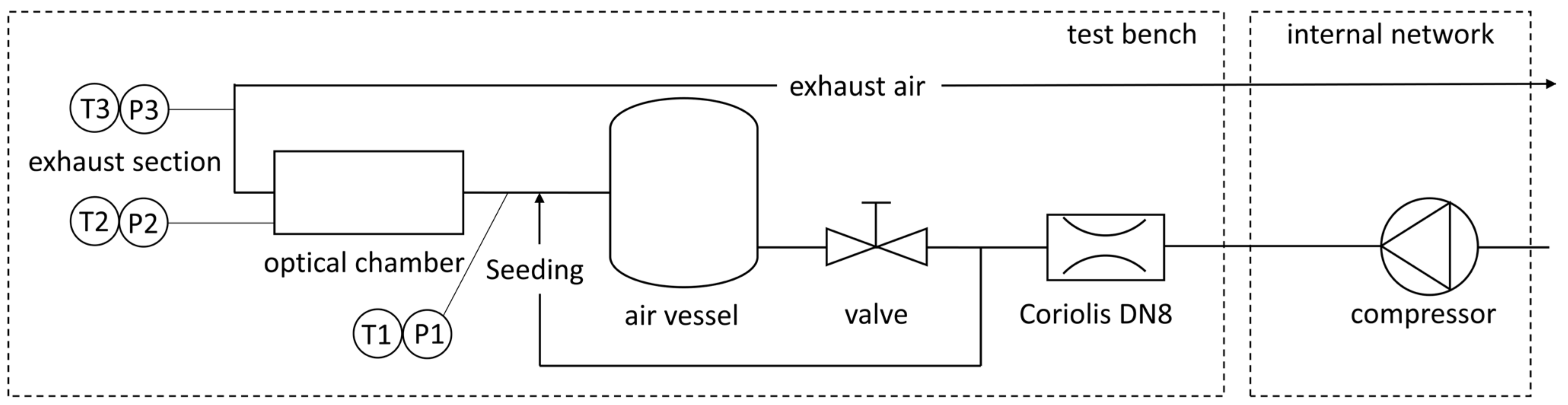
3.1. Experimental Facility

For the flow analysis of the interaction phenomena of two parallel intake valves, as well as to prove the feasibility of the LES modelling and PIV measurement techniques, a real engine geometry of Engine B at RWTH Aachen was designed as Optical Test Bench 2.1 (OTB 2.1). The main differences between OTB 2.1 and the previously presented OTB 1 [70] are the dual-intake valve setup instead of a single-valve setup and the real engine geometry instead of a simplified one. As shown in Figure 1, the inlet valve and intake pipe geometry of Engine B were used. The most important specifications of the single cylinder engine (SCE) of TME are shown in

Table 1. Specifications of the Single Cylinder Engine of TME (Engine B).

Description	Value	SI Units
Compression ratio	10.8	-
Stroke	90.5	mm
Bore	75	mm
Piston displacement	400	cm3

.

The geometry of the two intake channels, where the redirecting part of them is 3D printed, is shown in Figure 2 on the right-hand side. The valve lifts of the two valves can be adjusted independently up to a maximum valve lift of 9 mm. The mass flow rate is measured with a Coriolis mass flow meter, where the maximum total mass flow rate through both valves is about 120 kg/h, which is derived from measurements at Engine B.

Figure 2 (left) shows the dual-valve setup with an angle of 5° for better visualisation by preventing the first valve from casting a “shadow” over the second. As shown in Figure 3 in the middle, the optical chamber is located on a table. The inlet valve is rotated with the flow direction being upwards. The section has a width of 130 mm, and the inlet channels have a total length of 500 mm to ensure a fully developed flow.

Various temperature and pressure measurement tools are located at the beginning of the inlet channel, immediately downstream of the optical chamber, and at the outlet, where the optical chamber is connected to the environment with a 1 m-long outlet section. The temperature and pressure sensors as well as the outlet section remain unchanged from the previous study [70]. The used measuring devices and sensors are listed in

Table A1. Overview of measuring devices with the corresponding ranges and uncertainties.

Measurement	Measuring Device	Range	Uncertainty
Pressures P1, P2, P3	PD-39S/1178	$0\dots 5 \mathrm{b}\mathrm{a}\mathrm{r}$	0.1% full scale max
Mass flow rate	Endress + Hauser Promass 63 F DN8	$0\dots 437.5 \mathrm{k}\mathrm{g}/\mathrm{h}$	$\pm \left[0.5+\left(\frac{0.1\mathrm{k}\mathrm{g}/\mathrm{h}}{\mathrm{m}\mathrm{e}\mathrm{a}\mathrm{s}\mathrm{u}\mathrm{r}\mathrm{e}\mathrm{d} \mathrm{v}\mathrm{a}\mathrm{l}\mathrm{u}\mathrm{e}}\right)\cdot 100\right]\%$ of the measurement
Temperatures T1, T2, T3	Thermocouple Type K	$-40\dots 333 °\mathrm{C}$	$\pm 2.5 °\mathrm{C}$

in Appendix A.

Figure 4 shows the piping and instrumentation diagram (P&ID). Air at a pressure of 8 bar from the FHNW internal network is used as the air supply. The air flow is regulated by a valve. A Coriolis DN8 mass flow meter is used to measure the mass flow rate. Possible pressure oscillations are dampened using a 20-L air vessel. The by-pass air flow generates the tracer particles (liquid seeding). The fog is then diluted by the remaining air and enters the optical chamber through the two valves.

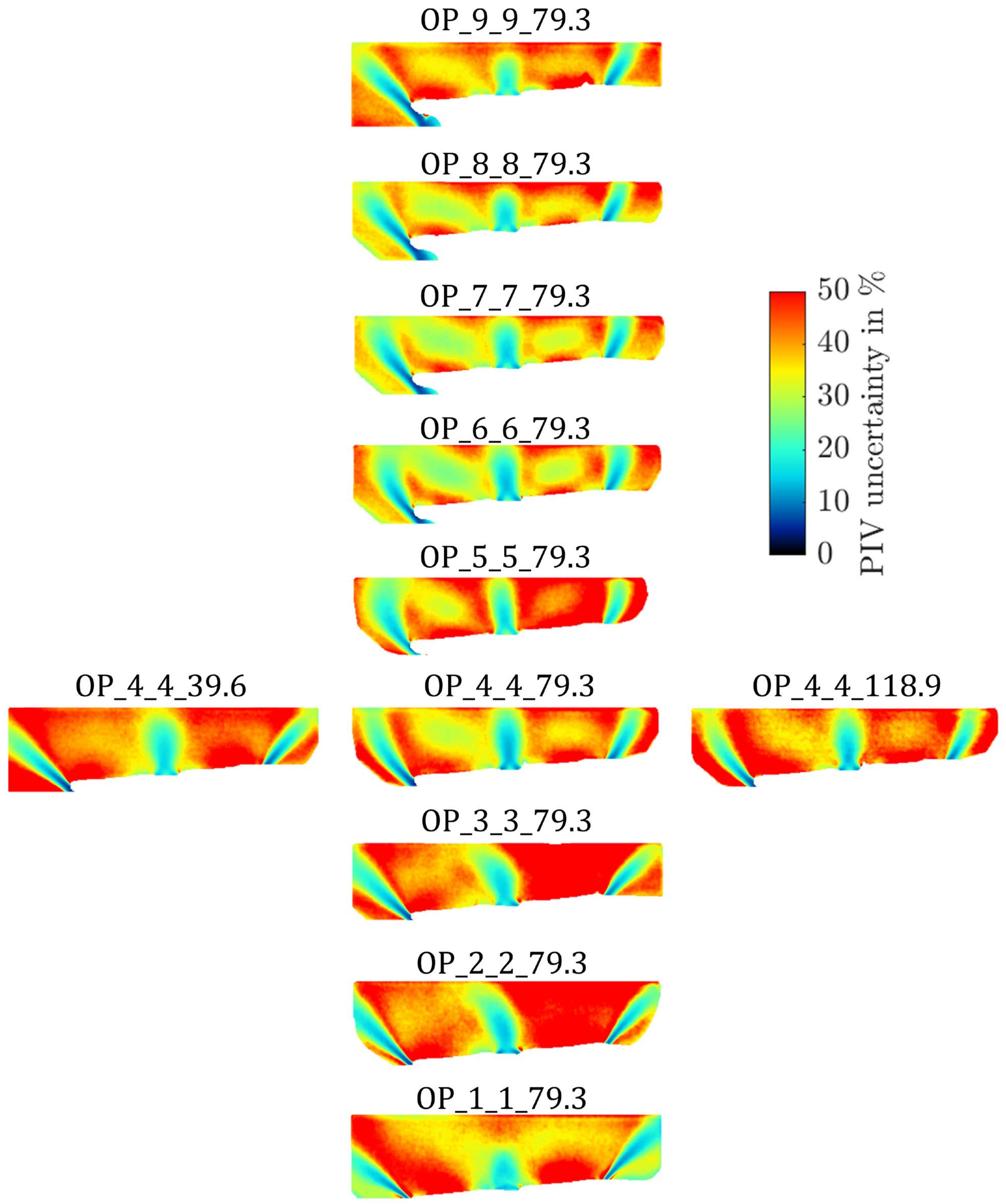
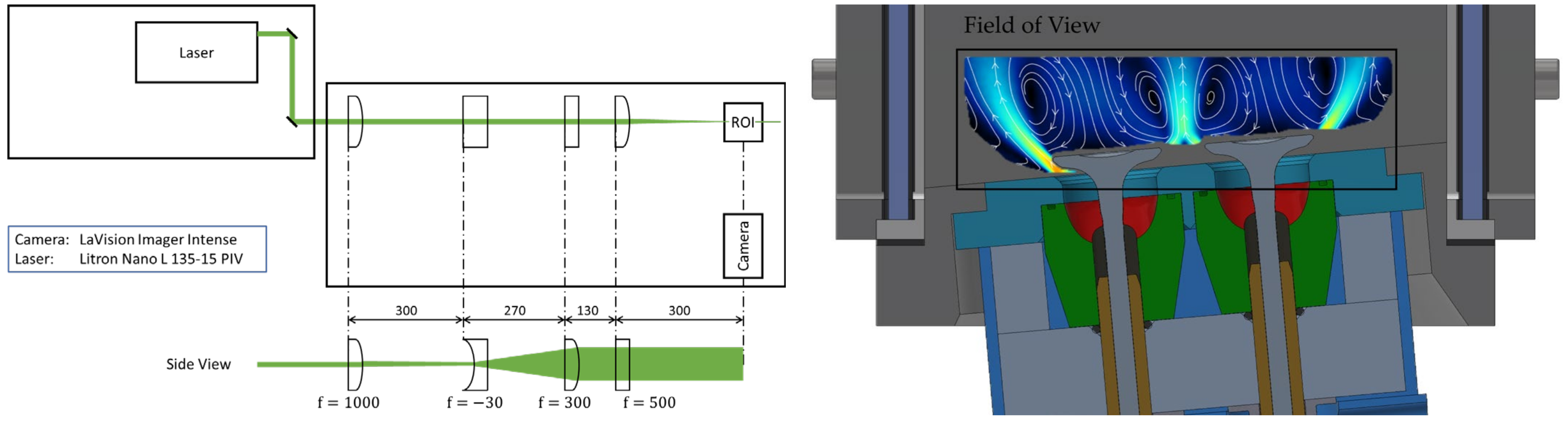
3.2. Optical Techniques and Image Processing

The measurement technique PIV is used and is described in the following section. Figure 5 shows the optical setup, where a Litron Nano L 135-15 PIV Nd:YAG laser with a pulse length of 6–9 ns, a wavelength of 532 nm, and an average energy of 135 mJ is utilized as a light source. The laser generates two beams, which are circular and have diameters of 5 mm. Mirrors are used to align the two beams to the optical chamber, and the first lens with a focal length of f = 1000 mm is utilised for focusing. To diverge the beam to the desired height, a cylindrical lens with f = −30 mm is used. After that, a second cylindrical lens with f = 300 mm is used for collimation. After that, the light sheet is focused once more perpendicular to the plane using another cylindrical lens with f = 500 mm, and the resulting light sheet is 30 mm high and 0.5 mm thick. To record the scattered light, a 12-bit charge-coupled device (CCD) camera (sensicam qe), commercially known as Imager Intense by LaVision, equipped with a 60 mm f/2.8 D AF Micro-NIKKOR objective, is used. The camera has a maximum operation frequency of 4 Hz in double-frame mode. The resolution of the chosen flow field is approximately 12.4 px/mm.

To record the scattered light, there must be tracer particles within the flow. Liquid seeding particles of approximately 1 µm are used as tracer particles, and the feed air is enriched with those using a Laskin nozzle aerosol generator, PivPart45 by PIVTEC. The used liquid seeding medium is SAFEX^® inside fog fluid flash/reflex B50, consisting of a non-toxic, highly pure polyol aerosol solution, as is commonly utilized in theatres. For modification of the particle density, the air mass flow rate through the aerosol generator can be adjusted.

Two laser pulses with a short time difference $\delta t$ are generated and spread into light sheets by the above-described optical components to illuminate a 2D plane of particles in the flow, which scatters their light. The camera records the scattered light as shown on the left-hand side in Figure 6. After that, the two raw double-images are divided into interrogation spots with typical sizes of 16 × 16 px, 32 × 32 px, or 64 × 64 px. The two exposures are then compared using an algorithm to identify the dominant flow direction by calculating the cross-correlation between the interrogation spot of exposure 1 and the proximate interrogation spots of exposure 2. This procedure is performed for the whole image, and a flow field can be calculated from this, as shown in Figure 6.

For the processing of the raw double-images, DaVis 10.1 is used, which is a commercially available software programme produced by LaVision. First, the local background noise is eliminated with an intensity normalisation filter. After that, a multi-pass, cross-correlation algorithm is used to calculate the local flow velocities. The two-dimensional vector fields have a height of 29 mm, a width of 108 mm, and a resolution of 0.4 mm, as shown on the right-hand side in Figure 6.

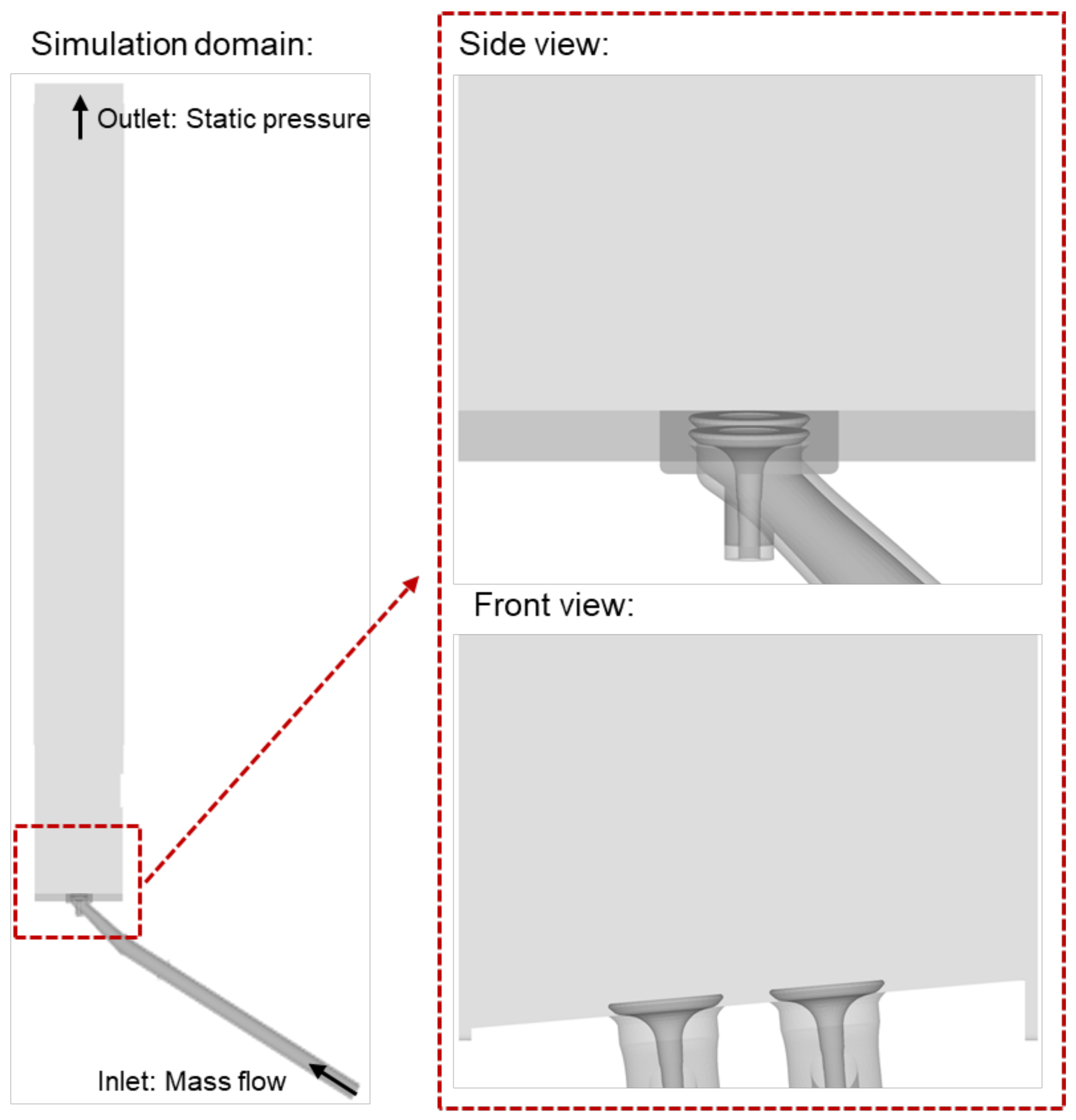
4. LES Model Description

Figure 7 shows the geometry and the simulation domain of the large eddy simulation (LES) model. Computational Fluid Dynamics (CFD) simulations were carried out with the Solver Converge v3.0. By default, a high-y+ approach was used to resolve the near-wall treatment. This high-y+ approach models the quantities inside the viscous sublayer and the buffer zone and resolves the flow field further away from the wall. The LES model “Dynamic Structure Model” was applied, which uses a one-equation approach for modelling the quantities in the sub-grid.

A convective CFL number of ${CFL}_{\mathrm{conv}}=1$ was chosen for resolving the flow field within the chosen grid accurately both in space and time. This ensured that the flow field quantities were calculated by the convective flow for the individual grid points.

The measured mass flow rate from the test rig with the two intake valves was chosen as the inlet boundary condition, together with the measured ambient temperature of $T_{\mathrm{in}}=293 \mathrm{K}$ and the fluid air. At the outlet, a measured ambient pressure and temperature of $p_{\mathrm{out}}=1.013 \mathrm{bar}$ and $T_{\mathrm{out}}=293 \mathrm{K}$ were specified. A non-moving fluid with $T_{\mathrm{ini}}=293 \mathrm{K}$ and $p_{\mathrm{ini}}=1.013 \mathrm{bar}$ was chosen as the initial condition. This made a certain response time necessary until quasi-stationary behaviour was apparent, which is discussed in the following text.

The mesh study was presented in the previous paper for a single-intake valve [70] (Chapter 4.2). The relative error of the discharge coefficient compared to the grid with the smallest cell dimension was evaluated for each of the five meshes. Based on this, a grid with a deviation in the discharge coefficient of less than 1% and a reasonable computational expense was chosen. Since the pressure range and mass flows in the present study are in the same ranges as for the previous one with the single-intake valve [70], the same meshing parameters were used.

A density-based, pressure-implicit split-operator (PISO) solver was used for the Navier–Stokes equations. For solving the governing equations (mass, momentum, and energy), CONVERGE offers the computationally less expensive pointwise successive over-relaxation (SOR) algorithm. CONVERGE recommends the SOR algorithm for engine simulations.

Table 2. SOR solver settings of convergence tolerance, minimum and maximum iterations, and the SOR relaxation value for the governing equations and the pressure.

	Convergence Tolerance	Min. Iterations	Max. Iterations	SOR Relaxation
Momentum	1 × 10−5	0	50	1.0
Pressure	1 × 10−8	2	500	1.1
Mass	1 × 10−4	0	2	1.0
Energy	1 × 10−4	0	2	1.0

shows convergence tolerances and the iteration limitations specified for the SOR algorithm.

To evaluate the convergence behaviour, the pressure drop across the two inlet valves is examined. To determine the pressure loss, numerical measuring points were inserted, one upstream of the inlet valves and another in the plenum further downstream. The transient behaviour already mentioned is present up to approximately 17.5 ms, according to Figure 8. Only the results in the range from 17.5 ms were used for time-averaging.

The operating points were chosen to have a trade-off between computational time and accuracy. According to this, three mass flow rates at 4 mm and valve lifts ranging from 2 mm to 8 mm with a step size of 2 mm at 79.3 kg/h were chosen. There were fewer valve lifts investigated using LES compared to PIV.

A comparison of the different operating points makes the results plausible. For the smallest valve lift of 2 mm, the largest pressure losses occur, whereas for the largest valve lift of 8 mm, the smallest pressure losses occur. It is also interesting to note that, from a valve lift of 4 mm, the pressure loss does not decrease appreciably, and at 6 mm, it is identical to that of 8 mm. At a constant valve lift, the pressure losses increase with an increasing mass flow rate. This is to be expected and makes the results plausible.

In addition, it can be noted that a pulsation of the pressure can be observed, in particular, for the operating points with 79.3 kg/h and valve lifts of 4, 6, and 8 mm and for a mass flow of 118.9 kg/h and a valve lift of 4 mm. The reason for the oscillating behaviour is flow separation around the intake valves, which is discussed in more detail in the following evaluation.

5. Results and Discussion

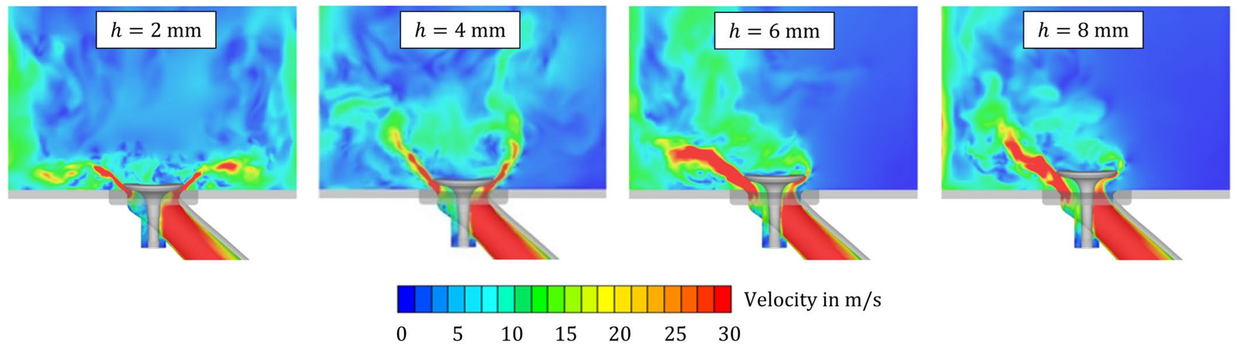
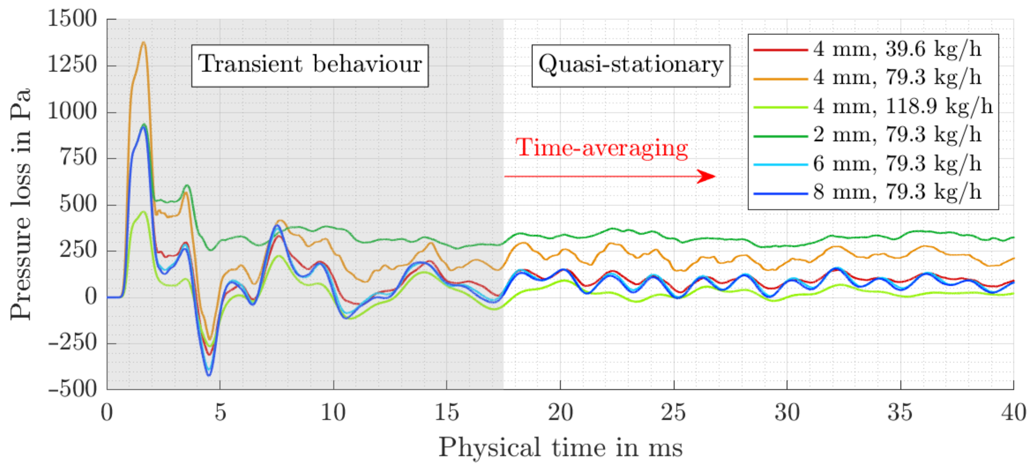
5.1. Flow Behaviour for the Different Operating Points

Figure 9 visualises the ensemble-averaged velocity fields calculated from 1000 individual fields of the particle image velocimetry (PIV) measurements, as well as the streamlines in white for the different operating points. The following example shows the nomenclature: OP_4_4_79.3, where the first number (4) corresponds to the valve lift of the left valve in millimetres, the second number (4) corresponds to the valve lift of the right valve in millimetres, and the third number (79.3) corresponds to the mass flow rate in kilograms per hour.

At a constant valve lift, as shown in Figure 9, the magnitude of the velocity increases with an increasing mass flow rate. The dominant flow structures are unaffected by the mass flow rate. The flow exiting the valves on the left- and right-hand sides form two outer jets, which are curved towards the valve side. The two outer jets are almost symmetrical to the vertical middle axis. Compared to this, two weaker interacting jets form in the middle and behave symmetrically. Besides this, the four jets cause recirculation zones on the side facing the valve, which are clearly visible in the streamlines. At 39.6 kg/h, there is a small difference compared to at 79.3 kg/h and 118.9 kg/h, where the two outer jets are straighter and not curved towards the middle. In contrast to the flow around an individual Flex-OeCoS valve [70], the results of the two Engine B intake valves are symmetrical. From this, it can be concluded that, for two intake valves, there is a smaller influence of the inclined surface on the flow behaviour.

The influence of the valve lift on the flow structure is significant compared to the mass flow rate. Starting from the highest valve lift of 9 mm, two straight outer jets to the right and left of the valves and a weaker interaction jet in the middle of the two valves form. Each of the jets causes a recirculation zone towards the valves. As the valve lift decreases to 5 mm, the middle jet strengthens, and the two outer jets bend towards the middle. The curvature of the two outer jets again decreases, while the valve lift decreases further to a value of 3 mm. Besides this, the middle jet is tilted to the left, which leads to a single recirculation region on the left-hand side of this interacting jet. This flow behaviour is caused by the inclined surface around the valves. The flow behaviour at a 2 mm valve lift is very similar to that at 3 mm. At a 1 mm valve lift, the two outer jets even curve away from the valve, while the inner interacting jets have a high velocity magnitude, but the region itself, which has two recirculation regions, is smaller.

An uncertainty study of the deviations arising from the PIV method was performed based on Sciacchitano Wieneke [90] and Wieneke [91] using DaVis software. For this purpose, the medians of all relative percentage deviations (absolute deviation divided by the respective individual velocity fields) were calculated for all operating points. The uncertainty of the operating point OP_4_4_79.3 is visualised in Figure 10. The PIV uncertainties for all operating points are shown in Appendix A in Figure A1. As expected, large velocity magnitudes lead to small deviations, and vice versa.

5.2. Validation of the LES

The large eddy simulations (LES) were validated with the time-averaged velocity fields obtained from PIV. About 900 timesteps were used to average the LES results, and approximately 1000 individual velocity fields were used to obtain the PIV results.

Figure 11 shows the variation in the mass flow rate ranging from 39.6 kg/h to 118.9 kg/h at a constant valve lift of 4 mm for the experimental (PIV) and simulation (LES) results. LES can depict the flow behaviour based on the mass flow variation very well, which means that there is very good agreement in the time-averaged velocity values of the LES compared to the PIV results. Even the smaller curvature of the two outer jets at a mass flow rate of 39.6 kg/h can be captured by both the LES and PIV results.

The variation in the valve lift in the range of 2 mm to 6 mm at a constant mass flow rate of 79.3 kg/h by means of the averaged velocity fields obtained from LES and PIV is visualised in Figure 12. In general, the LES results agree well with the PIV results in a qualitative manner, especially at 4 mm and 6 mm. For a valve lift of 2 mm, LES shows a good agreement in a qualitative way. However, there are some minor deviations in the middle jet, where the two jets of both valves interact with each other, and in the fluctuations of the outer jets.

5.3. Flow Analysis by LES

Based on the validation of LES performed with the optical PIV investigations, the flow field in the three-dimensional LES is now investigated in more detail. For this purpose, a representation by means of iso-surfaces in Figure 13 is used to visualise the flow structure. The areas in red represent a velocity of 30 m/s. The individual images were recorded at 35 ms in the quasi-stationary range.

The flow structure is analysed for the valve lift variation because it is unaffected by the mass flow rate. For a valve lift of 2 mm, a full flow separation is present. Due to the small valve lift and the geometry of the inlet channel, the discharge angle is very acute. In addition, Figure 13, on the right-hand side, shows a strong interaction between the flows leaving the two inlet valves due to the acute discharge angle. Due to the interaction, this suggests a high turbulence formation in this area.

With an increase in the valve lift to 4 mm, a full flow separation around the entire valve circumference can still be observed, but the discharge angle for this operating point is already significantly larger. Accordingly, the interaction between the two outgoing flows is not as intensive as with the smaller valve lift.

For a valve lift of 6 mm, there is now no longer any full detachment, and the flow detaches only via the left side of the two inlet valves. In the iso-representation, there is no flow over the right side. The shift in outflow due to the larger valve lift can be explained by the fact that the pressure drop decreases with larger valve lifts. This has already been quantified in the previous chapter. The resistance to outflow via the right side at relatively large valve lift values is high.

The propagation of the flow is also shown in Figure 14. The main amount of velocity, and thus also the larger part of the mass flow, flows over the left side, whereas only a small part flows over the right side of the inlet valve, which is attracted to the left side due to the higher flow velocities and the associated lower pressure. This results in the characteristic kinking of the free jet for valve lifts of 6 mm and 8 mm. The outflow angle corresponds approximately to that of 4 mm.

For the 8 mm valve lift, the outflow behaviour is very similar to that at a valve lift of 6 mm. Here, too, the detachment takes place via the left-hand side of the intake valves. The almost identical behaviour also corresponds to the pressure evaluations from the previous chapters, in which the pressure curves for 6 mm and 8 mm were found to be identical.

Based on the stationary investigations, the first conclusions can be drawn about the formation of tumble in a combustion engine. The initial phase of the valve lift (2 mm and 4 mm) does not contribute to the tumble formation. On the one hand, this is because there is a stronger interaction between the two intake valves; on the other hand, there is a comparable outflow on both sides, resulting in a rotating tumble movement. For the valve lifts of 6 mm and 8 mm, there is a one-sided outflow, which would result in a rotating tumble movement in a combustion engine. It can thus be stated that small valve lifts do not contribute to the formation of tumble, only larger valve lifts, and thus a one-sided outflow.

Figure 14. Planar side view through one intake valve with the velocity distribution for the valve lift variation.

Figure 14. Planar side view through one intake valve with the velocity distribution for the valve lift variation.

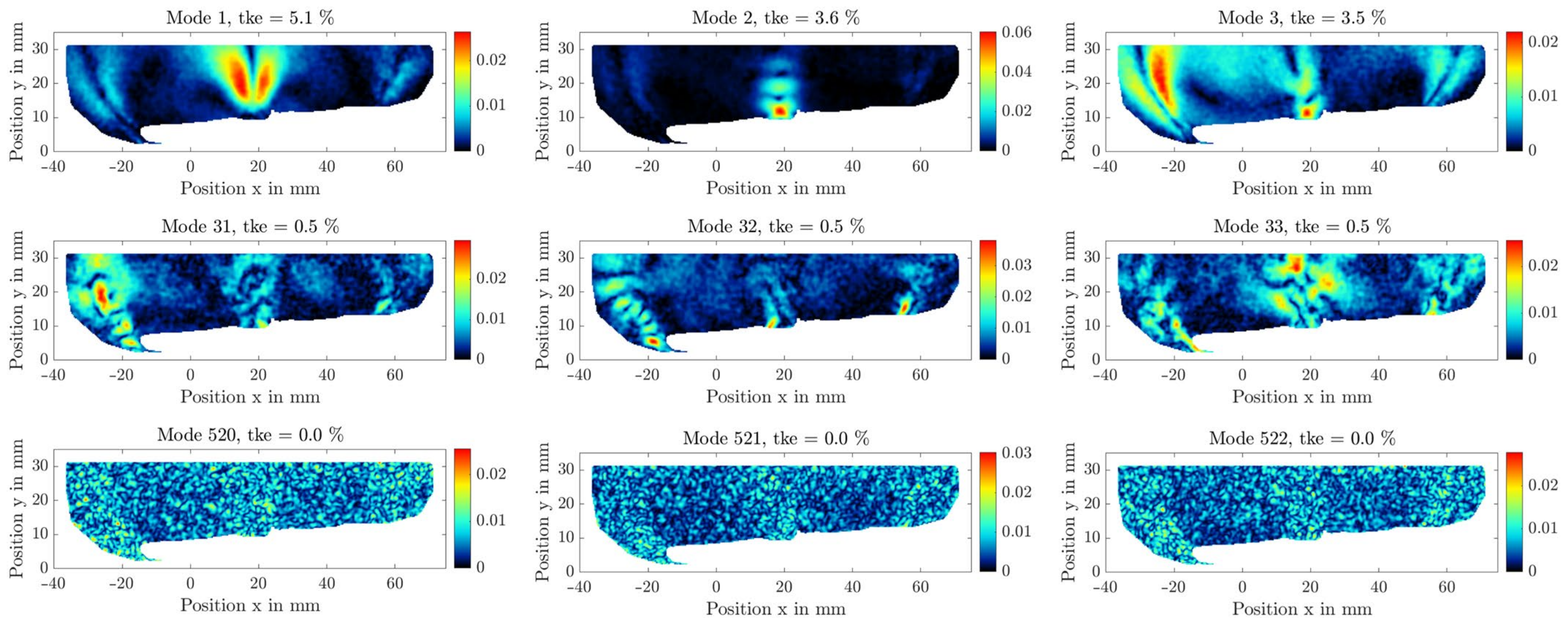
5.4. Proper Orthogonal Decomposition (POD) of PIV Measurements and Turbulent Structures

The cut-off modes between dominant, coherent, and turbulent structures are defined by means of the Relevance index $R_i$, the skewness coefficient $S_i$ and the flatness coefficient $T_i$ from Equations (8)–(10). Some exemplary modes of the operating point at 4 mm, 4 mm, and 79.3 kg/h of the different flow structures are shown in Figure 15, with each of them showing a certain flow structure. It has to be noted that the proper orthogonal decomposition (POD) modes are sorted according to their turbulent kinetic energies. Because of that, the first few modes contain the largest amounts of energy. The POD modes in Figure 15 visualise the correlations at different points of the flow. Two points within the red region in one mode are the most correlated.

Some exemplary time coefficients of the POD modes shown in Figure 15 are plotted in Figure 16. The amplitudes of the fluctuations within the time coefficients decrease with increasing POD mode numbers. The reason for this behaviour is that the small flow structures, which have high mode numbers, have low amounts of energy. A reduced-order model of the velocity fluctuations can be built using POD by summing up over a certain number of modes multiplied by their time coefficients.

Figure 17 visualises the amount of turbulent kinetic energy $\mathrm{tke}$ within the dominant, coherent, turbulent, and remaining POD modes for all operating points. For every operating point, the turbulent kinetic energy is highest within the dominant modes and decreases over the dominant, coherent, and turbulent modes. This division is found to be universal. The turbulent kinetic energy shows a quadratic increase with an increasing mass flow rate (left-hand side of Figure 17) or decreasing valve lift (right-hand side of Figure 17).

The dominant, coherent, and turbulent flow structures are visualised in Figure 18. These results were obtained by summing up the respective POD modes multiplied by the time coefficients over the dominant, coherent, and turbulent POD modes according to the cut-off modes. Nevertheless, this is only a qualitative comparison regarding the flow behaviour owing to the different image sections, the false vectors in the individual velocity fields, and the different total numbers of modes for the different operating points.

The dominant structures on the left-hand side in Figure 18 represent the largest and most energetic structures. The dominant structures are mainly located in the vicinity of the jets because turbulent energy is induced by shear layers. The reason for the dominant structures being particularly present in the middle jets could be the jet interactions. Compared to the dominant structures, the coherent ones are smaller and less energetic; these are shown in the middle in Figure 18. Like the dominant structures, the coherent structures are more dominant in the vicinity of the jets, but they can be observed throughout the whole flow field. The turbulent structures on the right-hand side of Figure 18 consist of lots of very small, homogeneously distributed structures across the whole flow area.

5.5. Reynolds Stress Transport at 79.3 kg/h and 4 mm

The different terms for ${\tau }_{xx}$ in the specific Reynolds stress transport equation are shown in Figure 19 for the operating point at 4 mm valve lifts and a 79.3 kg/h mass flow rate. The rows in Figure 19 correspond to the different terms in the equation, and the columns correspond to different calculation methods. The PIV results are shown on the left-hand side, where a two-dimensional evaluation is applied, since only the $x$- and $y$-velocity components are available, and the terms involving the third dimension $z$ are assumed to be zero. Two calculations were performed for the LES results, a two-dimensional one (middle) and a three-dimensional one, as presented on the right-hand side of Figure 19. Unlike in the PIV results, pressure data are also available for the LES results and the diffusion due to pressure–velocity fluctuations $D_{PVF,ij,}$ and the pressure–strain term ${\mathsf{\Pi }}_{ij}$ can be calculated.

The transient term ${\mathrm{T}}_{ij}$ corresponds to the first row in Figure 19, where the LES results have a small timestep of $5\cdot {10}^{-5} \mathrm{s}$. Therefore, the two- and three-dimensional LES results are suitable for predicting the transient term, but due to the large timesteps of the PIV, the ${\mathrm{T}}_{ij}$ is highly underpredicted. The second and third rows show the convective term $C_{ij}$ and the diffusion due to molecular transport $D_{MT,ij}$. Very good qualitative agreement between all three results can be seen in those terms. However, there is a difference in diffusion due to turbulent transport $D_{TT,ij}$ when comparing the two-dimensional and three-dimensional LES results. The differences are clearly recognisable in the vicinity of the jet. Nevertheless, the two-dimensional LES and PIV results agree very well with each other in a qualitative manner. In addition, the magnitude of the PIV result is slightly larger compared to the LES result. The reason for this could be the LES modelling, where the smallest eddies are modelled and not resolved. When looking at the diffusion due to pressure–velocity fluctuations $D_{PVF,ij}$ and the pressure–strain term ${\mathsf{\Pi }}_{ij}$, it is noticeable that these two terms only differ in terms of their signs. Since these two terms cancel each other out, it can be concluded that the deviation $\partial p^{\prime }/\partial x$ must be negligibly small. Besides this, there are larger areas with equal magnitudes in the three-dimensional calculation in comparison to the two-dimensional one. There is good agreement in the two-dimensional results (LES and PIV) of the production term $P_{ij}$. However, there is a difference between the two- and three-dimensional LES results, so the $z$-component of the velocity must be included to fit the production term $P_{ij}$ appropriately. The dissipation term $E_{ij}$ in the last row is smaller based on the LES results compared to the PIV results, which means that $E_{ij}$ is underpredicted in the LES calculation. The reason for this could be the LES modelling, but the two- and three-dimensional LES results agree very well with each other.

Since the PIV results only cover two dimensions and there are clear differences between the two- and three-dimensional calculations (LES) in the terms $D_{TT,ij}$ and $P_{ij}$, only a qualitative statement of the specific Reynolds stress transport equations is possible when using the PIV results. In addition, no local pressure data are captured during the PIV measurements, which means that not all terms can be calculated. There are also some limitations when using the LES results. The terms $D_{TT,ij}$ and $E_{ij}$ in Figure 19 show underpredictions compared to the corresponding PIV results. Due to the limitations of the PIV and LES results, direct numerical simulations (DNS) would probably enable the quantification of the respective terms in the specific Reynolds stress transport equations.

6. Conclusions and Outlook

6.1. Conclusions

The test bench presented by Hoffmann et al. [70] was modified so that the intake ports and two intake valves were based on the single-cylinder engine (SCE) of TME at RWTH Aachen University. The aim was to represent the flow conditions of an internal combustion engine (ICE) with the properties of a common commercial passenger vehicle engine and to analyse these experimentally and numerically. Optical experiments with particle image velocimetry (PIV) were performed using this test rig, and large eddy simulations (LES) were conducted, including a validation of the developed model. Different valve lifts and mass flow rates were investigated experimentally and numerically, whereby the simulations were validated with the PIV results using the intake valve plane.

6.1.1. Flow Behaviour Depending on the Mass Flow Rate and the Valve Lift

Analogous to the results from Hoffmann et al. [70], the results with the dual valves show that the flow structures are unaffected by the mass flow rate at a constant valve lift of 4 mm, and only the magnitude of the velocity increases with an increasing mass flow rate. In comparison to that, the flow structures are affected by the valve lift at a constant mass flow rate of 79.3 kg/h. In general, two outer jets and a middle jet, which result from the interacting flows of the two valves, are formed. Starting at a 9 mm valve lift, there is a weak interaction jet in the middle of the two valves. This jet strengthens with a decreasing valve lift to 5 mm. For 2 mm and 3 mm, the interacting jet is tilted to the left because of the inclined surface. The velocity magnitude of the middle jet is the highest with a 1 mm valve lift. The two outer jets leave the valve straight, and with a decreasing valve lift to 5 mm, the jets bend towards the middle. The curvature of the outer jets decreases until the jets are straight again at valve lifts of 2 mm and 3 mm. At 1 mm, the outer jets curve away from the valve. The validation of the LES with the PIV results shows good qualitative agreement for flow behaviour.

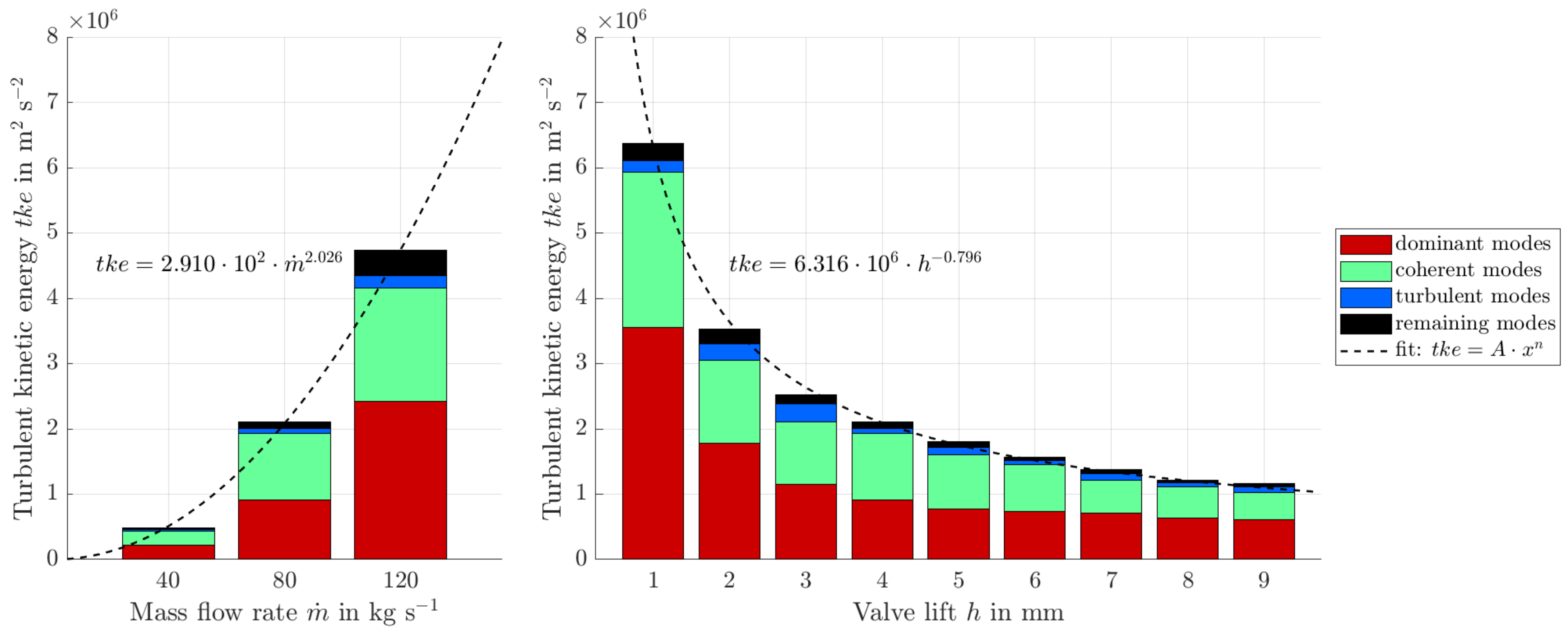
6.1.2. Structures and Turbulent Kinetic Energy

In addition, the turbulent structures were analysed by employing the proper orthogonal decomposition (POD) and, furthermore, the quadruple decomposition, where the PIV velocity fields are split into their mean values and the fluctuations within the dominant, coherent, and turbulent structures. The dominant structures are large and highly energetic and are particularly present in the vicinity of the jets leaving the valves. The turbulent structures are the smallest and least energetic. They are homogenously distributed throughout the whole flow field. The splitting of the energy into dominant, coherent, and turbulent structures is almost equal (universal) for each operating point. There is a quadratic increase in the turbulent kinetic energy inside the whole flow field with an increasing mass flow rate and a decreasing valve lift.

6.1.3. Reynolds Stress Transport Equation

The Reynolds stress transport equation is used to identify the dominant terms of convection $C_{ij}$, diffusion due to turbulent transport $D_{TT,ij}$, diffusion due to pressure–velocity fluctuations $D_{PVF,ij}$, production $P_{ij}$, and pressure–strain ${\mathsf{\Pi }}_{ij}$, which are more than one order of magnitude larger compared to the other terms. Compared to these, the transient term, the diffusion due to molecular transport and the dissipation terms $T_{ij}$, $D_{MT,ij}$, and $E_{ij}$ are negligible. Since the specific Reynolds stress transport equation is calculated from the PIV and LES results, the limitations of both can be identified. Because of the small timesteps, $T_{ij}$ can be predicted using LES. Moreover, pressure and three-dimensional velocity data are available from the LES results and can be used to perform two- and three-dimensional Reynolds stress analyses. The three-dimensional LES calculation shows that two dimensions are not sufficient to predict the terms $D_{TT,ij}$ and $P_{ij}$. Therefore, employing the stereo-PIV, which captures the third velocity component as well, would greatly enhance the Reynolds stress term evaluations. There are also some limitations in using the LES results, as the terms $D_{TT,ij}$ and $E_{ij}$ are underpredicted compared to the PIV results. Due to the limitations of the PIV and LES results, the specific Reynolds stress transport equation evaluation only allows a qualitative analysis.

6.2. Outlook

The inflow event through the intake valves, as shown in Section 1.1, has a significant influence on the early flame kernel growth and, therefore, on the efficiency of the combustion process. The optical and numerical methodologies presented in this paper offer the opportunity to investigate the intake valve flow in detail for future ICEs. Further analysis of the flow separation at intake valves with temporal highly resolved optical PIV measurements should clarify whether the LES methodology is able to resolve the flow separations in terms of amplitude and frequency accordingly. Furthermore, the investigation of the transient valve lift is of great interest as it is closer to engine-like conditions. With these two tasks accomplished, it should be possible to understand the flow behaviour of the intake valves and their statistic behaviour under the variation of the valve lift speed (engine speed) and boost pressure in depth. With these, control strategies or geometry changes of the intake port or intake valves should be applied to achieve a reproducible inflow event. This is signified by a lower variability in the inflow velocity and the corresponding turbulence level.

References

1. Reitz, R.D.; Ogawa, H.; Payri, R.; Fansler, T.; Kokjohn, S.; Moriyoshi, Y.; Agarwal, A.; Arcoumanis, D.; Assanis, D.; Bae, C.; et al. IJER editorial: The future of the internal combustion engine. Int. J. Engine Res. 2020, 21, 3–10. [Google Scholar] [CrossRef]
2. International Energy Agency (IEA). World Energy Outlook 2019. Available online: https://www.iea.org/reports/world-energy-outlook-2019 (accessed on 21 June 2023).
3. Karwade, A.; Thombre, S. Implementation of thermal and fuel stratification strategies to extend the load limit of HCCI engine. J. Therm. Sci. Technol. 2019, 14, JTST0020. [Google Scholar] [CrossRef]
4. Young, M.B. Cyclic Dispersion–Some Quantitative Cause-and-Effect Relationships; SAE International: Warrendale, PA, USA, 1980. [Google Scholar] [CrossRef]
5. Young, M.B. Cyclic Dispersion in the Homogeneous-Charge Spark-Ignition Engine—A Literature Survey; SAE International: Warrendale, PA, USA, 1981. [Google Scholar] [CrossRef]
6. Ozdor, N.; Dulger, M.; Sher, E. Cyclic Variability in Spark Ignition Engines a Literature Survey; SAE International: Warrendale, PA, USA, 1994. [Google Scholar] [CrossRef]
7. Ozdor, N.; Dulger, M.; Sher, E. An Experimental Study of the Cyclic Variability in Spark Ignition Engines; SAE International: Warrendale, PA, USA, 1996. [Google Scholar] [CrossRef]
8. Ball, J.K.; Raine, R.R.; Stone, C.R. Combustion analysis and cycle-by-cycle variations in spark ignition engine combustion Part 2: A new parameter for completeness of combustion and its use in modelling cycle-by-cycle variations in combustion. Proc. Inst. Mech. Eng. Part D J. Automob. Eng. 1998, 212, 507–523. [Google Scholar] [CrossRef]
9. Galloni, E. Analyses about parameters that affect cyclic variation in a spark ignition engine. Appl. Therm. Eng. 2009, 29, 1131–1137. [Google Scholar] [CrossRef]
10. Granet, V.; Vermorel, O.; Lacour, C.; Enaux, B.; Dugué, V.; Poinsot, T. Large-Eddy Simulation and experimental study of cycle-to-cycle variations of stable and unstable operating points in a spark ignition engine. Combust. Flame 2012, 159, 1562–1575. [Google Scholar] [CrossRef]
11. Urushihara, T.; Murayama, T.; Takagi, Y.; Lee, K.-H. Turbulence and Cycle-by-Cycle Variation of Mean Velocity Generated by Swirl and Tumble Flow and Their Effects on Combustion; SAE International: Warrendale, PA, USA, 1995. [Google Scholar] [CrossRef]
12. Stiehl, R.; Bode, J.; Schorr, J.; Krüger, C.; Dreizler, A.; Böhm, B. Influence of intake geometry variations on in-cylinder flow and flow–spray interactions in a stratified direct-injection spark-ignition engine captured by time-resolved particle image velocimetry. Int. J. Engine Res. 2016, 17, 983–997. [Google Scholar] [CrossRef]
13. Bode, J.; Schorr, J.; Krüger, C.; Dreizler, A.; Böhm, B. Influence of three-dimensional in-cylinder flows on cycle-to-cycle variations in a fired stratified DISI engine measured by time-resolved dual-plane PIV. Proc. Combust. Inst. 2017, 36, 3477–3485. [Google Scholar] [CrossRef]
14. Bode, J.; Schorr, J.; Krüger, C.; Dreizler, A.; Böhm, B. Influence of the in-cylinder flow on cycle-to-cycle variations in lean combustion DISI engines measured by high-speed scanning-PIV. Proc. Combust. Inst. 2019, 37, 4929–4936. [Google Scholar] [CrossRef]
15. Hasse, C. Scale-resolving simulations in engine combustion process design based on a systematic approach for model development. Int. J. Engine Res. 2016, 17, 44–62. [Google Scholar] [CrossRef]
16. Fischer, J.; Kettner, M.; Spicher, U.; Velji, A. Zylinderinnenströmung und zyklische Schwankungen bei Benzin-Direkteinspritzung. MTZ-Mot. Z. 2005, 66, 202–209. [Google Scholar] [CrossRef]
17. Heywood, J.B. Internal Combustion Engine Fundamentals, 2nd ed.; McGraw-Hill Education: New York, NY, USA, 2018; Available online: https://www.accessengineeringlibrary.com/content/book/9781260116106 (accessed on 12 March 2023).
18. Huang, R.F.; Lin, K.H.; Yeh, C.-N.; Lan, J. In-cylinder tumble flows and performance of a motorcycle engine with circular and elliptic intake ports. Exp. Fluids 2009, 46, 165–179. [Google Scholar] [CrossRef]
19. Kapitza, L.; Imberdis, O.; Bensler, H.P.; Willand, J.; Thévenin, D. An experimental analysis of the turbulent structures generated by the intake port of a DISI-engine. Exp. Fluids 2010, 48, 265–280. [Google Scholar] [CrossRef]
20. Bari, S.; Saad, I. CFD modelling of the effect of guide vane swirl and tumble device to generate better in-cylinder air flow in a CI engine fuelled by biodiesel. Comput. Fluids 2013, 84, 262–269. [Google Scholar] [CrossRef]
21. Wang, T.; Li, W.; Jia, M.; Liu, D.; Qin, W.; Zhang, X. Large-eddy simulation of in-cylinder flow in a DISI engine with charge motion control valve: Proper orthogonal decomposition analysis and cyclic variation. Appl. Therm. Eng. 2015, 75, 561–574. [Google Scholar] [CrossRef]
22. Krishna, A.S.; Mallikarjuna, J.M.; Kumar, D. Effect of engine parameters on in-cylinder flows in a two-stroke gasoline direct injection engine. Appl. Energy 2016, 176, 282–294. [Google Scholar] [CrossRef]
23. Yang, J.; Dong, X.; Wu, Q.; Xu, M. Effects of enhanced tumble ratios on the in-cylinder performance of a gasoline direct injection optical engine. Appl. Energy 2019, 236, 137–146. [Google Scholar] [CrossRef]
24. Ramajo, D.; Zanotti, A.; Nigro, N. In-cylinder flow control in a four-valve spark ignition engine: Numerical and experimental steady rig tests. Proc. Inst. Mech. Eng. Part D J. Automob. Eng. 2011, 225, 813–828. [Google Scholar] [CrossRef]
25. Vu, T.-T.; Guibert, P. Proper orthogonal decomposition analysis for cycle-to-cycle variations of engine flow. Effect of a control device in an inlet pipe. Exp. Fluids 2012, 52, 1519–1532. [Google Scholar] [CrossRef]
26. Jemni, M.A.; Kantchev, G.; Abid, M.S. Influence of intake manifold design on in-cylinder flow and engine performances in a bus diesel engine converted to LPG gas fuelled, using CFD analyses and experimental investigations. Energy 2011, 36, 2701–2715. [Google Scholar] [CrossRef]
27. Agarwal, A.K.; Gadekar, S.; Singh, A.P. In-cylinder air-flow characteristics of different intake port geometries using tomographic PIV. Phys. Fluids 2017, 29, 95104. [Google Scholar] [CrossRef]
28. Lumley, J.L. Early Work on Fluid Mechanics in the IC Engine. Annu. Rev. Fluid Mech. 2001, 33, 319–338. [Google Scholar] [CrossRef]
29. Perini, F.; Miles, P.C.; Reitz, R.D. A comprehensive modeling study of in-cylinder fluid flows in a high-swirl, light-duty optical diesel engine. Comput. Fluids 2014, 105, 113–124. [Google Scholar] [CrossRef]
30. Clark, L.G.; Kook, S.; Chan, Q.N.; Hawkes, E. The Effect of Fuel-Injection Timing on In-cylinder Flow and Combustion Performance in a Spark-Ignition Direct-Injection (SIDI) Engine Using Particle Image Velocimetry (PIV). Flow Turbul. Combust. 2018, 101, 191–218. [Google Scholar] [CrossRef]
31. Krishna, B.M.; Mallikarjuna, J.M. Comparative study of in-cylinder tumble flows in an internal combustion engine using different piston shapes—An insight using particle image velocimetry. Exp. Fluids 2010, 48, 863–874. [Google Scholar] [CrossRef]
32. Harshavardhan, B.; Mallikarjuna, J.M. Effect of piston shape on in-cylinder flows and air-fuel interaction in a direct injection spark ignition engine—A CFD analysis. Energy 2015, 81, 361–372. [Google Scholar] [CrossRef]
33. Liu, K.; Haworth, D.C. Large-Eddy Simulation for an Axisymmetric Piston-Cylinder Assembly with and without Swirl. Flow Turbul. Combust. 2010, 85, 279–307. [Google Scholar] [CrossRef]
34. Rabault, J.; Vernet, J.A.; Lindgren, B.; Alfredsson, P.H. A study using PIV of the intake flow in a diesel engine cylinder. Int. J. Heat Fluid Flow 2016, 62, 56–67. [Google Scholar] [CrossRef]
35. El-Adawy, M.; Heikal, M.R.; Aziz, A.R.A.; Siddiqui, M.I.; Wahhab, H.A.A. Experimental study on an IC engine in-cylinder flow using different steady-state flow benches. Alex. Eng. J. 2017, 56, 727–736. [Google Scholar] [CrossRef]
36. Liu, D.; Wang, T.; Jia, M.; Wang, G. Cycle-to-cycle variation analysis of in-cylinder flow in a gasoline engine with variable valve lift. Exp. Fluids 2012, 53, 585–602. [Google Scholar] [CrossRef]
37. Clenci, A.C.; Iorga-Simăn, V.; Deligant, M.; Podevin, P.; Descombes, G.; Niculescu, R. A CFD (computational fluid dynamics) study on the effects of operating an engine with low intake valve lift at idle corresponding speed. Energy 2014, 71, 202–217. [Google Scholar] [CrossRef]
38. Wang, T.; Liu, D.; Tan, B.; Wang, G.; Peng, Z. An Investigation into In-Cylinder Tumble Flow Characteristics with Variable Valve Lift in a Gasoline Engine. Flow Turbul. Combust. 2015, 94, 285–304. [Google Scholar] [CrossRef]
39. Borée, J.; Miles, P.C. In-Cylinder Flow. In Encyclopedia of Automotive Engineering; John Wiley & Sons, Ltd.: Chichester, UK, 2014; pp. 1–31. [Google Scholar] [CrossRef]
40. Vester, A.K.; Nishio, Y.; Alfredsson, P.H. Investigating swirl and tumble using two prototype inlet port designs by means of multi-planar PIV. Int. J. Heat Fluid Flow 2019, 75, 61–76. [Google Scholar] [CrossRef]
41. Vermorel, O.; Richard, S.; Colin, O.; Angelberger, C.; Benkenida, A.; Veynante, D. Towards the understanding of cyclic variability in a spark ignited engine using multi-cycle LES. Combust. Flame 2009, 156, 1525–1541. [Google Scholar] [CrossRef]
42. Liu, K.; Haworth, D.C.; Yang, X.; Gopalakrishnan, V. Large-eddy Simulation of Motored Flow in a Two-valve Piston Engine: POD Analysis and Cycle-to-cycle Variations. Flow Turbul. Combust. 2013, 91, 373–403. [Google Scholar] [CrossRef]
43. Chen, C.; Ameen, M.M.; Wei, H.; Iyer, C.; Ting, F.; Vanderwege, B.; Som, S. LES Analysis on Cycle-to-Cycle Variation of Combustion Process in a DISI Engine; SAE International: Warrendale, PA, USA, 2019. [Google Scholar] [CrossRef]
44. Corcione, F.E.; Valentino, G. Analysis of in-cylinder flow processes by LDA. Combust. Flame 1994, 99, 387–394. [Google Scholar] [CrossRef]
45. Chan, V.S.S.; Turner, J.T. Velocity measurement inside a motored internal combustion engine using three-component laser Doppler anemometry. Opt. Laser Technol. 2000, 32, 557–566. [Google Scholar] [CrossRef]
46. Janas, P.; Wlokas, I.; Böhm, B.; Kempf, A. On the Evolution of the Flow Field in a Spark Ignition Engine. Flow Turbul. Combust. 2017, 98, 237–264. [Google Scholar] [CrossRef]
47. Freudenhammer, D.; Baum, E.; Peterson, B.; Böhm, B.; Jung, B.; Grundmann, S. Volumetric intake flow measurements of an IC engine using magnetic resonance velocimetry. Exp. Fluids 2014, 55, 1724. [Google Scholar] [CrossRef]
48. El-Adawy, M.; Heikal, M.R.; Aziz, A.R.A.; Adam, I.K.; Ismael, M.A.; Babiker, M.E.; Baharom, M.B.; Firmansyah; Abidin, E.Z.Z. On the Application of Proper Orthogonal Decomposition (POD) for In-Cylinder Flow Analysis. Energies 2018, 11, 2261. [Google Scholar] [CrossRef]
49. Bücker, I.; Karhoff, D.-C.; Klaas, M.; Schröder, W. Stereoscopic multi-planar PIV measurements of in-cylinder tumbling flow. Exp. Fluids 2012, 53, 1993–2009. [Google Scholar] [CrossRef]
50. Baum, E.; Peterson, B.; Surmann, C.; Michaelis, D.; Böhm, B.; Dreizler, A. Investigation of the 3D flow field in an IC engine using tomographic PIV. Proc. Combust. Inst. 2013, 34, 2903–2910. [Google Scholar] [CrossRef]
51. Cao, J.; Ma, Z.; Li, X.; Xu, M. 3D proper orthogonal decomposition analysis of engine in-cylinder velocity fields. Meas. Sci. Technol. 2019, 30, 85304. [Google Scholar] [CrossRef]
52. Enaux, B.; Granet, V.; Vermorel, O.; Lacour, C.; Pera, C.; Angelberger, C.; Poinsot, T. LES study of cycle-to-cycle variations in a spark ignition engine. Proc. Combust. Inst. 2011, 33, 3115–3122. [Google Scholar] [CrossRef]
53. Leudesdorff, W.; Unger, T.; Janicka, J.; Hasse, C. Scale-resolving Simulations for Combustion Process Development. MTZ Worldw. 2019, 80, 62–67. [Google Scholar] [CrossRef]
54. Graftieaux, L.; Michard, M.; Grosjean, N. Combining PIV, POD and vortex identification algorithms for the study of unsteady turbulent swirling flows. Meas. Sci. Technol. 2001, 12, 1422–1429. [Google Scholar] [CrossRef]
55. Voisine, M.; Thomas, L.; Borée, J.; Rey, P. Spatio-temporal structure and cycle to cycle variations of an in-cylinder tumbling flow. Exp. Fluids 2011, 50, 1393–1407. [Google Scholar] [CrossRef]
56. Chen, H.; Reuss, D.L.; Sick, V. On the use and interpretation of proper orthogonal decomposition of in-cylinder engine flows. Meas. Sci. Technol. 2012, 23, 85302. [Google Scholar] [CrossRef]
57. Chen, H.; Reuss, D.L.; Hung, D.L.S.; Sick, V. A practical guide for using proper orthogonal decomposition in engine research. Int. J. Engine Res. 2013, 14, 307–319. [Google Scholar] [CrossRef]
58. Li, Y.; Zhao, H.; Peng, Z.; Ladommatos, N. Tumbling flow analysis in a four-valve spark ignition engine using particle image velocimetry. Int. J. Engine Res. 2002, 3, 139–155. [Google Scholar] [CrossRef]
59. Joo, S.H.; Srinivasan, K.K.; Lee, K.C.; Bell, S.R. The behaviourt of small- and large-scale variations of in-cylinder flow during intake and compression strokes in a motored four-valve spark ignition engine. Int. J. Engine Res. 2004, 5, 317–328. [Google Scholar] [CrossRef]
60. Reeves, M.; Garner, C.; Dent, J.; Halliwell, N. Study of barrel swirl in a four-valve optical IC engine using particle image velocimetry. In Proceedings of the COMODIA: Third International Symposium on Diagnostics and Modeling of Combustion in Internal Combustion Engines, Yokohama, Japan, 11–14 July 1994. [Google Scholar]
61. Cosadia, I.; Borée, J.; Charnay, G.; Dumont, P. Cyclic variations of the swirling flow in a Diesel transparent engine. Exp. Fluids 2006, 41, 115–134. [Google Scholar] [CrossRef]
62. Vester, A.K.; Nishio, Y.; Alfredsson, P.H. Unravelling tumble and swirl in a unique water-analogue engine model. J. Vis. 2018, 21, 557–568. [Google Scholar] [CrossRef] [PubMed]
63. Wahono, B.; Setiawan, A.; Lim, O. Experimental study and numerical simulation on in-cylinder flow of small motorcycle engine. Appl. Energy 2019, 255, 113863. [Google Scholar] [CrossRef]
64. El Adawy, M.; Heikal, M.R.; Aziz, A.R.A. Experimental Investigation of the in-Cylinder Tumble Motion inside GDI Cylinder at Different Planes under Steady-State Condition using Stereoscopic-PIV. J. Appl. Fluid Mech. 2019, 12, 41–49. [Google Scholar] [CrossRef]
65. Bottone, F.; Kronenburg, A.; Gosman, D.; Marquis, A. Large Eddy Simulation of Diesel Engine In-cylinder Flow. Flow Turbul. Combust. 2012, 88, 233–253. [Google Scholar] [CrossRef]
66. Nishad, K.; Ries, F.; Li, Y.; Sadiki, A. Numerical Investigation of Flow through a Valve during Charge Intake in a DISI-Engine Using Large Eddy Simulation. Energies 2019, 12, 2620. [Google Scholar] [CrossRef]
67. Ramajo, D.E.; Nigro, N.M. In-Cylinder Flow Computational Fluid Dynamics Analysis of a Four-Valve Spark Ignition Engine: Comparison Between Steady and Dynamic Tests. J. Eng. Gas Turbine Power 2010, 132, 052804. [Google Scholar] [CrossRef]
68. Richard, S.; Dulbecco, A.; Angelberger, C.; Truffin, K. Invited Review: Development of a one-dimensional computational fluid dynamics modeling approach to predict cycle-to-cycle variability in spark-ignition engines based on physical understanding acquired from large-eddy simulation. Int. J. Engine Res. 2015, 16, 379–402. [Google Scholar] [CrossRef]
69. Hasse, C.; Sohm, V.; Durst, B. Detached eddy simulation of cyclic large scale fluctuations in a simplified engine setup. Int. J. Heat Fluid Flow 2009, 30, 32–43. [Google Scholar] [CrossRef]
70. Hoffmann, J.; Mirsch, N.; Vera-Tudela, W.; Wüthrich, D.; Rosenberg, J.; Günther, M.; Pischinger, S.; Weiss, D.A.; Herrmann, K. Flow Field Investigation of a Single Engine Valve Using PIV, POD, and LES. Energies 2023, 16, 2402. [Google Scholar] [CrossRef]
71. Keskinen, J.-P.; Vuorinen, V.; Kaario, O.; Larmi, M. Large eddy simulation of a piston–cylinder assembly: The sensitivity of the in-cylinder flow field for residual intake and in-cylinder velocity structures. Comput. Fluids 2015, 122, 123–135. [Google Scholar] [CrossRef]
72. Keskinen, J.-P.; Vuorinen, V.; Kaario, O.; Larmi, M. Large Eddy Simulation of the Intake Flow in a Realistic Single Cylinder Configuration; SAE International: Warrendale, PA, USA, 2012. [Google Scholar] [CrossRef]
73. Antila, E.; Imperato, M.; Kaario, O.; Larmi, M. Effect of Intake Channel Design to Cylinder Charge and Initial Swirl; SAE International: Warrendale, PA, USA, 2010. [Google Scholar] [CrossRef]
74. Guo, Y.Z.; Kui, H.L.; Shao, C.S.; Wang, Z.Z.; Liu, Y. Flow Characteristics of a Dual-Intake Port Diesel Engine with Guide Vanes. J. Appl. Fluid Mech. 2022, 15, 709–722. [Google Scholar] [CrossRef]
75. El-Adawy, M.; Heikal, M.; Aziz, A.A.; Siddiqui, M.; Munir, S. Characterization of the Inlet Port Flow under Steady-State Conditions Using PIV and POD. Energies 2017, 10, 1950. [Google Scholar] [CrossRef]
76. Gugulothu, S.K.; Reddy, K.H.C. CFD Simulation of In-Cylinder Flow on Different Piston Bowl Geometries in a DI Diesel Engine. J. Appl. Fluid Mech. 2016, 9, 1147–1155. [Google Scholar] [CrossRef]
77. Giannakopoulos, G.K.; Frouzakis, C.E.; Boulouchos, K.; Fischer, P.F.; Tomboulides, A.G. Direct numerical simulation of the flow in the intake pipe of an internal combustion engine. Int. J. Heat Fluid Flow 2017, 68, 257–268. [Google Scholar] [CrossRef]
78. Kang, K.Y.; Reitz, R.D. The effect of intake valve alignment on swirl generation in a DI diesel engine. Exp. Therm. Fluid Sci. 1999, 20, 94–103. [Google Scholar] [CrossRef]
79. Lee, K.; Bae, C.; Kang, K. The effects of tumble and swirl flows on flame propagation in a four-valve S.I. engine. Appl. Therm. Eng. 2007, 27, 2122–2130. [Google Scholar] [CrossRef]
80. Choe, S.G.; Choe, T.H.; Ho, I.C.; Mun, M.H.; Kim, I.J.; Ri, J.H.; Jong, R.U.; Kim, Y.C. Effect of the geometrical shapes of the helical-spiral shroud intake valve on swirl generation in cylinder of diesel engine. Results Eng. 2023, 18, 101132. [Google Scholar] [CrossRef]
81. Qiao, J.; Liu, J.; Zhang, Q.; Liang, J.; Wang, R.; Zhao, Y.; Shen, D. Experimental investigation on the effects of Miller cycle coupled with asynchronous intake valves on the performance of a high compression ratio GDI engine. Fuel 2023, 332, 126088. [Google Scholar] [CrossRef]
82. Qiao, J.; Liu, J.; Liang, J.; Jia, D.; Wang, R.; Shen, D.; Duan, X. Experimental investigation the effects of Miller cycle coupled with asynchronous intake valves on cycle-to-cycle variations and performance of the SI engine. Energy 2023, 263, 125868. [Google Scholar] [CrossRef]
83. Teodosio, L.; Pirrello, D.; Berni, F.; De Bellis, V.; Lanzafame, R.; D’Adamo, A. Impact of intake valve strategies on fuel consumption and knock tendency of a spark ignition engine. Appl. Energy 2018, 216, 91–104. [Google Scholar] [CrossRef]
84. Versteeg, H.K.; Malalasekera, W. An Introduction to Computational Fluid Mechanics, 6th ed.; John Wiley & Sons: New York, NY, USA, 2009. [Google Scholar]
85. Weiss, J. A Tutorial on the Proper Orthogonal Decomposition. In AIAA Aviation 2019 Forum; American Institute of Aeronautics and Astronautics: Reston, VA, USA, 2019. [Google Scholar] [CrossRef]
86. Druault, P.; Delville, J.; Bonnet, J. Experimental 3D Analysis of the Large Scale Behaviour of a Plane Turbulent Mixing Layer. Flow Turbul. Combust. 2005, 74, 207–233. [Google Scholar] [CrossRef]
87. Roudnitzky, S.; Druault, P.; Guibert, P. Proper orthogonal decomposition of in-cylinder engine flow into mean component, coherent structures and random Gaussian fluctuations. J. Turbul. 2006, 7, N70. [Google Scholar] [CrossRef]
88. Rulli, F.; Fontanesi, S.; d’Adamo, A.; Berni, F. A critical review of flow field analysis methods involving proper orthogonal decomposition and quadruple proper orthogonal decomposition for internal combustion engines. Int. J. Engine Res. 2021, 22, 222–242. [Google Scholar] [CrossRef]
89. Wu, S.; Patel, S.; Ameen, M. Investigation of Cycle-to-Cycle Variations in Internal Combustion Engine Using Proper Orthogonal Decomposition. Flow Turbul. Combust. 2022, 110, 125–147. [Google Scholar] [CrossRef]
90. Sciacchitano, A.; Wieneke, B. PIV uncertainty propagation. Meas. Sci. Technol. 2016, 27, 084006. [Google Scholar] [CrossRef]
91. Wieneke, B.F.A. PIV Uncertainty Quantification and Beyond. Ph.D. Thesis, Delft University of Technology, Delft, The Netherlands, 2017. [Google Scholar]
Figure 1. Uptake pipe geometry of Engine B (left), computer-aided design (CAD) drawing of the intake valves and uptake pipes of OTB 2.1 (right).
Energies 16 06917 g001
Figure 2. Optical chamber with the dual-intake valves from Engine B with up to 9 mm of valve lift (left) and 3D-printed dual-intake pipes reproducing the Engine B geometry (right).
Energies 16 06917 g002
Figure 3. Cross-sectional view of the optical chamber (left), test rig with the measurement positions (middle), and a picture of the test rig (right). The pressure and temperature measurements are indicated with P1, P2, and P3 and T1, T2, and T3, respectively.  m ˙  is used to show the mass flow rate measurement.
Energies 16 06917 g003
Figure 4. Piping and instrumentation diagram (P&ID) of the optical test rig with two intake valves, showing the pressure supply, measurement equipment, air vessel, seeding implementation, optical chamber, and exhaust section.
Energies 16 06917 g004
Figure 5. Optical setups for the low-speed PIV (@4 Hz) including a Litron Nano L 135-15 PIV Nd:YAG laser (left); field of view with dimensions of approximately 108 mm × 29 mm showing the flow around the two valves (right).
Energies 16 06917 g005
Figure 6. Exemplary raw double-images (left), individual velocity fields (middle), and time-averaged velocity field (right).
Energies 16 06917 g006
Figure 7. Region of interest marked by a red dashed box with two intake valves and a flow separation region (left). Side and front views on both intake valves and the flow separation region (right).
Energies 16 06917 g007
Figure 8. Pressure loss over both intake valves for all six operating points with a marked transient area and quasi-stationary area for time averaging.
Energies 16 06917 g008
Figure 9. Ensemble-averaged velocity fields (colour bar) and streamlines (white arrows) for different mass flow rates and valve lifts; nomenclature: OP_4_4_79.3 = 4 mm valve lift of the left valve, 4 mm valve lift of the right valve, and 79.3 kg/h mass flow.
Energies 16 06917 g009
Figure 10. Median of the percentage of PIV uncertainty in the instantaneous velocity fields of the operating point OP_4_4_79.3 = 4 mm valve lift of the left valve, 4 mm valve lift of the right valve, and a mass flow rate of 79.3 kg/h.
Energies 16 06917 g010
Figure 11. Time-averaged velocity fields of the mass flow variation at a constant valve lift of 4 mm for LES (left) and PIV (right).
Energies 16 06917 g011
Figure 12. Time-averaged velocity fields of the valve lift variation at a constant mass flow rate of 79.3 kg/h for LES (left) and PIV (right).
Energies 16 06917 g012
Figure 13. Side view (left) and top view (right) of both intake valves with the flow structure represented by the iso-surface of the velocity for the valve lift variation.
Energies 16 06917 g013
Figure 15. POD modes computed from PIV velocity fields representing the dominant, coherent, and turbulent structures for the operating points of 4 mm, 4 mm, and 79.3 kg/h.
Energies 16 06917 g015
Figure 16. Time coefficients of modes 1, 31, and 520 for the operating point of 4 mm, 4 mm, and 79.3 kg/h computed from the PIV measurements.
Energies 16 06917 g016
Figure 17. Amount of turbulent kinetic energy  t k e  within the dominant, coherent, turbulent, and remaining modes of the mass flow variation at a constant valve lift of 4 mm for both valves (left) and the valve lift variation at a constant mass flow rate of 79.3 kg/h (right).
Energies 16 06917 g017
Figure 18. Cumulative dominant (left), coherent (middle), and turbulent (right) structures obtained from the POD quadruple decomposition for the operating points at 4 mm, 4 mm, and 79.3 kg/h.
Energies 16 06917 g018
Figure 19. Components of  x x  of the specific Reynolds stress transport equations at 4 mm, 4 mm, and 79.3 kg/h computed from PIV (left), 2D LES (middle), and 3D LES (right) (terms involving the third dimension  z  are assumed to be zero for the 2D calculations).
Energies 16 06917 g019