Abstract
In this paper, ensemble-based machine learning models with gradient boosting machine and random forest are proposed for predicting the power production from six different solar PV systems. The models are based on three year’s performance of a 1.2 MW grid-integrated solar photo-voltaic (PV) power plant. After cleaning the data for errors and outliers, the model features were chosen on the basis of principal component analysis. Accuracies of the developed models were tested and compared with the performance of models based on other supervised learning algorithms, such as k-nearest neighbour and support vector machines. Though the accuracies of the models varied with the type of PV systems, in general, the machine learned models developed under the study could perform well in predicting the power output from different solar PV technologies under varying working environments. For example, the average root mean square error of the models based on the gradient boosting machines, random forest, k-nearest neighbour, and support vector machines are 17.59 kW, 17.14 kW, 18.74 kW, and 16.91 kW, respectively. Corresponding averages of mean absolute errors are 8.28 kW, 7.88 kW, 14.45 kW, and 6.89 kW. Comparing the different modelling methods, the decision-tree-based ensembled algorithms and support vector machine models outperformed the approach based on the k-nearest neighbour method. With these high accuracies and lower computational costs compared with the deep learning approaches, the proposed ensembled models could be good options for PV performance predictions used in real and near-real-time applications.
1. Introduction
As part of the worldwide initiatives for addressing the climate change [1] and long-term energy security challenges, policies and programs are implemented for increasing the share of sustainable energy resources in the global power sector. With an estimated global installed capacity of 228 GW by 2022 [2], solar energy would play a major role in this emerging clean energy scenario. Improvements in the conversion efficiencies and reduction in the unit costs [3,4,5], along with the implementation of incentive mechanisms such as feed-in tariff and net metering [3], makes solar PV an attractive renewable energy option for large scale deployments.
As solar resources are stochastic, power developed by the PV systems fluctuates considerably, even within short time spans. Power prediction models for the PV plants, which correlate relevant weather variables, viz., solar insolation, wind speed, relative humidity, ambient temperature, etc. [6,7,8,9], with the system output is essential for understanding and managing these temporal variations in the generation. Popular tools used for such predictions are based on generalized physical equations. These models often may not fully capture the effects of site-dependent parameters. In the case of solar PV powerplants with sufficient operational data, machine learning (ML) techniques can effectively be employed for correlating the weather parameters with the PV system performance.
Machine learning methods are being successfully used in understanding modelling energy resources and systems. Considering the specific application of predicting solar PV power output, ML algorithms based on non-linear regression, such as support vector machine [SVM] [1,3,10,11] k-nearest neighbour [k-NN] [3,12], Markov chain [13], etc., have been proposed. These models, which are relatively simpler and computationally light, shows moderate accuracies when used for solar PV power predictions [3]. To further enhance the model performance, deep learning algorithms, such as artificial neural networks [ANNs], are widely used [14,15,16,17,18,19] for the prediction schemes. For improving the model accuracy, advanced modelling methods based on extreme learning machine [ELM] with single layer feed forward neural network has been suggested in [20]. For learning long-term details in sequences and to extract features from the time series power data, the radiation classification coordinate [RCC] method is also being applied in a long short-term memory [LSTM] models as reported in [21]. Nevertheless, ANN-based models may have instability issues in a relatively smaller data set [11]. With small changes in the input data sets, this could result in significant variations in the predictions [11,22]. Further, these approaches are computationally demanding and may not be suitable for applications where real-time or near-real-time predictions are needed.
Compared with individual learners, ensemble-based ML techniques generally perform better, as they could overcome the above limitation [16,17]. They are computationally lighter compared with complex deep learning algorithms [23,24,25] and, hence, are suitable for real time prediction applications. In view of these advantages, some of the recent studies [1,26,27] proposed ensemble-based ML models, such as random forests [RF] and gradient boosted regression trees [GBM], for solar PV power prediction. Nevertheless, compared with other methods, ensemble-based models are relatively less explored in solar power forecasting. For example, in some recent reviews and evaluations on PV power forecasting [28,29], no studies on decision-tree-based ensembled algorithms are reported.
In this study, we propose ensemble machine learning models for predicting the power output from six different solar photovoltaic technologies operating under tropical environments. Accuracies of these models are then compared with methods based on supervised learning algorithms, such as SVM and kNN, which were reported in our earlier paper [3].
Compared with the previous investigations in this area, the present study has the following novel features:
1. In contrast to the previous studies which mostly consider a single type of PV system, we present prediction models for six different PV systems, covering both the first- and second-generation PV technologies, working under the same operating weather conditions.
2. While several reported studies are based on PV systems of smaller sizes, performance data from a 1.2 MW well-instrumented and grid-integrated solar PV power plant is used for developing and testing the proposed models.
3. Substantial performance data, covering three years of commercial operation of the plant and collected at high resolution of 1 min, are used for the model development and testing.
After this introductory section, ensemble machine learning methods used in this study are introduced. The methodology adopted for the development of the models are then discussed, highlighting the features of the experimental solar farm and the descriptions on the pre-processing of the data. Selection of model features and its optimal structure are also discussed. Finally, performance of the models is presented and discussed along with the salient conclusions of the study.
2. Ensemble Machine Learning Methods
The ensemble-based machine learning methods used in this study are random forest (RF) and gradient boosting machine (GBM). These methods are briefly explained in the following sections. Details of SVM and kNN, which were used for the comparison, can be found in our previous paper [3].
2.1. Gradient Boosting Machine
In the gradient boosting machine (GBM) technique, predictions from several decision trees are integrated together for generating the final predictions. By implementing gradient descent in function space, GBMs construct a forward stage-wise addictive model [30]. The direction of the steepest descent is like gradient descent in parameter space, and the mth iteration can be given by the negative gradient of the loss function [30]:
By taking a step along this direction, it will eventually reduce the loss. At each iteration, to predict the negative gradient, a regression tree model will be fitted into the model. As a result, a surrogate loss is used in the squared error. For determination of the step length ρm, further effort is necessary, as the negative gradient gives only the direction of the step. Line search [31] can be performed by:
2.2. Random Forest
Random forest is a tree-based ensemble machine learning technique based on the classification and regression trees (CART) method [32,33,34,35]. In developing a CART model, initially a model is constructed through a growing step by recursive partitioning of the set of observations, choosing the best “split” to divide the current set of observations in two subsets, minimizing the local internal variance of the response [36]. Here, a split is defined by a variable and a threshold. To avoid the possibilities of overfitting, the CART model development performs a growing step, which is then followed by a pruning step. This approach suffers from the drawback of instability with respect to perturbations on the training data set. To overcome this issue, [32] introduced RF, where the search is limited to a random subset of input variables at each splitting node; thus, the tree could grow fully without pruning. RF makes use of bagging (bootstrap aggregation) to combine multiple random predictors in order to aggregate predictions, which improves the stability and accuracy of the model. This helps to avoid over-fitting and generalizing of the training data, thereby reducing variance. The number of input variables randomly chosen at each split, which is denoted as mtry, and the number of trees in the forest, which is represented as ntree, are the two main tuning parameters, and the algorithm is fairly robust to the choice of these values. The estimated output obtained by averaging the output of all trees can be expressed as
where k is the number of regression trees, X is the vectored input variable, and Ti (x) is a single regression tree constructed on the basis of a subset of input variables and the bootstrapped samples. The algorithm of RF for regression involves the following steps [33,37]: (1) Extract ntree bootstrap samples from the original data; (2) For each of these samples, randomly sample mtry predictors (variables) at each node, grow an unpruned classification or regression tree, and choose the best split among these variables; (3) Estimate the new data by aggregating the predictions of ntree trees (i.e., majority vote is used for classification, average is used for regression); and (4) For every bootstrap iteration, estimate the data which are not included in the bootstrap sample (“out-of-bag”, or OOB, data) using the tree grown with the bootstrap sample. For a tree grown on bootstrapped data, the OOB data can be used as a test set for that tree. The training is terminated when the OOB error stabilizes. The OOB error rate which corresponds to the prediction error for the OOB data is used in evaluating the quality of the fitted model. The OOB error is used to estimate the generalization ability of the model and serves as a type of internal cross validation. For each observation (Xi, Yi), an estimation of Yi is made by aggregating only the trees constructed over bootstrap samples not containing (Xi, Yi). The OOB error () can be expressed as
3. Development of the Models
Methodology adopted for developing the solar output prediction models using the proposed machine learning techniques and evaluating their performances are presented in Figure 1. Details of these are discussed in the following sections:
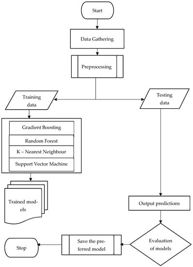
Figure 1.
Procedures for developing the proposed machine learning models.
3.1. Data Description
The data required for developing the proposed machine learning models are collected from Tenaga Suria Brunei (TSB) solar PV power plant in Brunei Darussalam. Configuration of the solar PV systems in the plant and data collection systems are shown in Figure 2. There are six different types of solar systems in the farm, which covers the first and second generations of solar PV technologies. These are (a) Single crystalline silicon (sc-Si), (b) Polycrystalline silicon (mc-Si), (c) Microcrystalline silicon (nc-Si/a-Si), (d) Amorphous silicon (a-Si), (e) Copper indium selenium (CIS), and (f) Hetero-junction with intrinsic thin layer (HIT). Each of these modules have the same peak capacity of 200 kW. Specifications of these are given in Table 1. As seen from the figure, two types of modules are jointly connected to a converter. Further, every two converters are connected to an inverter. Various operational data from the system, including the weather parameters and power output, are collected through sensors and data loggers. Data are sensed every second, which are then averaged into minute values for this study.
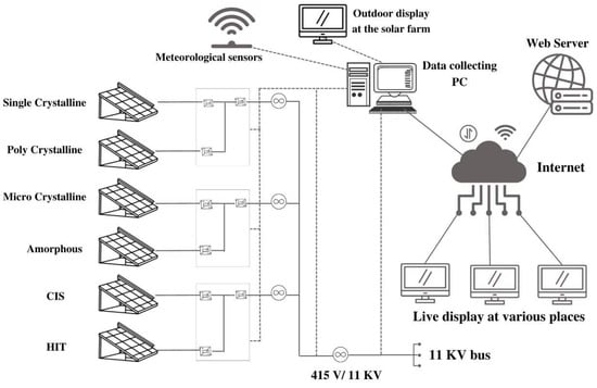
Figure 2.
Layout of the experimental solar farm.

Table 1.
Specification of the solar PV systems.
3.2. Data Pre-Processing and Feature Selection
The power data from different PV systems, corresponding to three years of operation of the power plant, were collected for the study. Along with this, corresponding weather parameters, such as solar insolation, ambient temperature, relative humidity, and wind velocity, were also collected. Being the most important weather parameter in solar PV conversion, monthly averaged total daily global solar insolation at the site is presented in Figure 3. As seen from the figure, the solar resource reaches its maximum of 6.32 kWh in the month of March and its minimum of 3.85 kWh in November. The annual averaged daily global insolation at the site is 4.97 kWh. This indicates the strong solar resource available at the site from the weather and power data thus collected; data corresponding to 0700 to 1700 h (productive day time) were filtered. These data were further cleaned to remove possible errors and outliers. Feature selection is an important step in the development of machine learning models, as irrelevant features may add noise to the model. Keeping this in view, the possibility of using principle component analysis (PCA), which is widely used for data dimensionality reduction, was considered in this study. In a trial considering the total output from the farm, the average mean absolute error (MAE) and root mean square error (RMSE) of the models were found to be reduced by 19.8% and 4.6%, respectively. Hence, the dimensionality of the models was reduced through PCA.
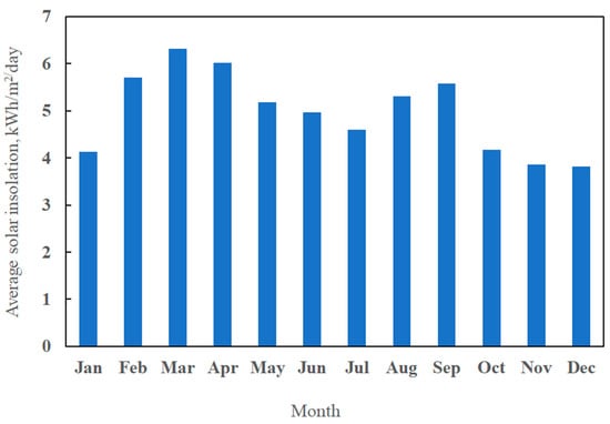
Figure 3.
Monthly averaged daily solar insolation at the power plant site.
PCA maximizes the correlation among the initial variables, thereby forming a new set of mutually orthogonal variables, namely principal components (PCs). Among the PCs in order, the first PC represents most of the variance in the data, and the subsequent ones account for the largest proportion of variability that has not been accounted for by its predecessors [38]. The eigenvalue test is used to retain the most significant principal components (PCs) which have eigenvalues greater than one [39]. The retained PCs are then rotated using varimax rotation. This ensures that each variable is maximally correlated with only one component and has a near zero association with the other components [40]. The factor loadings after the rotation reflects the contribution of the variables to a given PC as well as the similarity among the variables. A factor loading higher than 0.75 is considered as “strong”, 0.75–0.50 as “moderate”, and 0.49–0.30 as “weak”. High factor loading of a variable indicates its strong contribution to a particular PC [32]. On the basis of these criteria, two PCs (PC1 and PC2) were chosen for the model development. Solar irradiance and temperature were predominantly embedded in PC1, whereas the wind characteristics are reflected in PC2.
3.3. Model Features and Validation
The RF and GBM based solar PV power prediction models, as discussed above, were trained using the train data set. For minimizing the model bias and enhancing the model performance, k-fold cross-validation was performed, taking a k value of 10. The optimal GBM models thus developed had 100 trees with a learning rate of 0.100. Limit depth of individual trees was considered as 3. The RF models have regression random forests with 300 trees. Similarly, the SVM models, with which the performances of the GBM and RF approaches are compared, have radial kernels with cost function 1, gamma 0.5, epsilon 0.1, and number of support vectors 30. The KNN models of rectangular kernels with a k of 7 and Euclidean distance of 2 were also used for the comparison.
The optimal RF and GBM models thus developed were tested for accuracies with the test data set. Root Mean Square Error (RMSE), normalized root mean square error (NRMSE), Mean Absolute Error (MAE), and Coefficient of Determination (R2) were used as indices to evaluate the model performance [3,12], where
and
where N is the total number of datapoints, is the observed power, is the predicted power, and is the mean value of actual power. In addition, and are the maximum and minimum value of observed power, respectively.
4. Performance of the Models
The power predicted by the RF and GBM models for the six solar PV systems under varying operating environments are compared in Figure 4, Figure 5, Figure 6, Figure 7, Figure 8 and Figure 9. The solid lines represent the model predictions, whereas the scattered points are the observed power. Closeness of the points representing the observed power to the prediction line are indications of the model accuracies. As seen from the figures, both the RF and GBM models could perform well in estimating the power generation from different solar PV systems. Differences in the predicted and observed power vary with the PV technologies, with predictions for single and polycrystalline panels being closer to the actual measurements.
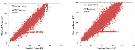
Figure 4.
Comparison of the power predicted by the ensembled models with the observed power for single crystalline PV system.
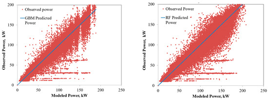
Figure 5.
Comparison of the power predicted by the ensembled models with the observed power for polycrystalline PV system.
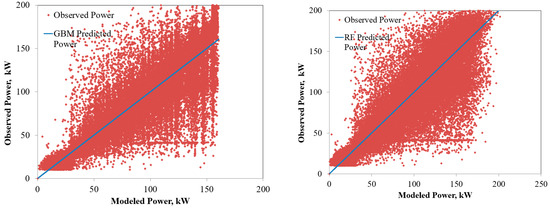
Figure 6.
Comparison of the power predicted by the ensembled models with the observed power for microcrystalline PV system.
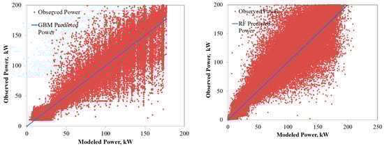
Figure 7.
Comparison of the power predicted by the ensembled models with the observed power for amorphous PV system.
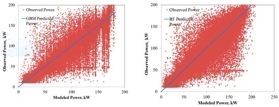
Figure 8.
Comparison of the power predicted by the ensembled models with the observed power for CIS PV system.
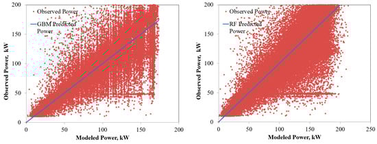
Figure 9.
Comparison of the power predicted by the ensembled models with the observed power for HIT PV system.
Further, for quantifying the model performances, errors between the predictions and observations were computed using the different error metrices defined in Section 3.3. On the basis of the same data, prediction models based on support vector machines (SVM) and k-nearest neighbour (kNN) were also developed and tested, as discussed in our previous study on this same solar PV plant, reported in [3]. These are then compared with the performance of the proposed ensembled models, as presented in Figure 10. Though the accuracies of the models vary with the panel type and the applied machine learning method, in general, all the ML models could reasonably capture the performance of the solar PV systems. For different panel types of 200 kWp rated capacity, the RMSEs of GBM and RF models ranged from 12.87 kW to 22.25 kW and from 13.46 kW to 22.93 kW, respectively. For these methods, corresponding average RMSEs over different PV technologies are 17.59 kW and 17.14 kW. For the models based on kNN and SVM, the RMSEs ranged from 14.75 kW to 24.20 kW and from 12.75 kW to 23.43 kW, respectively, for different PV technologies, with corresponding average errors of 18.74 kW and 16.91 kW. Similarly, considering the MAE, the error ranges for GBM-, RF-, kNN-, and SVM-based models are 6.06 kW to 10.18 kW, 5.61 kW to 9.64 kW, 13.33 kW to 15.73 kW, and 2.26 kW to 9.13 kW, respectively. Corresponding MAE values, averaged for different PV technologies, are 8.28 kW, 7.88 kW, 14.45 kW, and 6.89 kW, respectively. As seen from the figure, similar trends are observed in the case of the other error measures such as NRMSE and R2. These indicate that the models based on the ensembled and SVM-based algorithms outperformed the kNN-based predictions. However, the computational times required for the SVM-based models were substantially high compared with the ensembled models. This is because the training dataset consisted of two years of performance data from the farm (more than 1 million data points), and SVM has the inherent limitation of high computational time with larger large training samples. Performances of the proposed ensembled models are comparable with those of the modelling approaches based on deep learning, as reported, for example, in [14,15]. The lower computation demand of the proposed ensembled models compared with the SVM and complex deep learning options could be an advantage in applications requiring real-time and near-real-time power predictions.
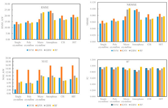
Figure 10.
Performance of the models in predicting the power production from the solar PV systems.
The modelled and observed power produced by the panels are compared in Figure 11. In order to clearly visualize the variations in the model performances, results from an hour of a representative day are plotted in the graph. The figures bring out the performance of the models under varying insulation levels and changing ambient temperatures. Close agreements between the predictions of the GBM, RF, and SVM models and actual observations are well evident in these figures as well. The relatively low accuracies of kNN-based models are well reflected in the figure. This is more prominent in the evening hours when the ambient temperature (which is used as the model input) starts receding while the cell temperature (which actually influences the efficiencies of the cells) still remains high due to the time lag in cooling the cell surfaces.
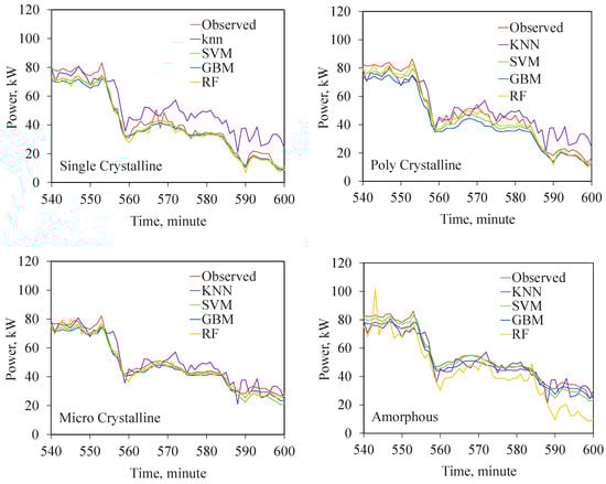
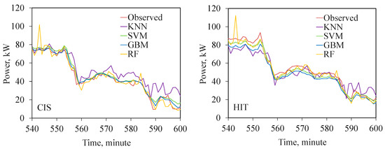
Figure 11.
Power output from different PV systems predicted by the ML models compared with the actual measurements.
5. Conclusions
In this paper, we present ensemble machine learning models based on random forest and gradient boosting machine algorithms to predict the power generation from six different PV technologies working under tropical environments. These are then compared with the performance of the similar models based on support vector machines and k-nearest neighbour, which were reported by the authors earlier. The data required for developing these models were collected from a well-instrumented 1.2 MW solar farm, which were then pre-processed for model development. Features of the model were chosen through principal component analysis. In general, models based on decision-tree-based ensembled algorithms performed well in predicting the power output from the solar panels with different technologies. For example, with a panel rated capacity of 200 kWp, the average RMSEs of the models based on the gradient boosting machines and random forest are 17.59 kW and 17.14 kW, respectively. The corresponding MAEs are 8.28 kW and 7.88 kW.
Being computationally less demanding compared with the deep learning models, the proposed ensembled models can be a good choice for system control applications which require real-time or near-real time production estimates. These prediction models can be further developed into solar PV power forecasting systems by integrating them with the forecasts of relevant weather inputs from numerical weather prediction (NWP) models. For example, depending on the time horizon of the relevant NWP weather forecasts (hour-ahead, day-ahead, etc.), which are used as the inputs for the proposed prediction models, the power generated by the PV plant can be forecasted in different time windows of interest. Such integrated forecasting systems can assist the grid managers in formulating efficient power dispatch strategies and help PV power plant developers in successfully participating in the dynamic energy markets.
Author Contributions
Conceptualization, V.R., H.Y., M.I.P., S.-Q.D. and M.S.; methodology, testing, and analysis, V.R., H.Y. and S.-Q.D.; interpretation of results and supervision, M.S. and M.I.P.; writing, V.R., H.Y., M.I.P. and S.-Q.D. All authors have read and agreed to the published version of the manuscript.
Funding
This research was funded by Universiti Brunei Darussalam, grant number UBD/RSCH/1.3/FICBF(a)/2022/006.
Data Availability Statement
Not applicable.
Acknowledgments
We thankfully acknowledge the Energy Department, the Prime Minister’s Office (EDPMO), Brunei Darussalam, for the support during the course of this study.
Conflicts of Interest
The authors declare no conflict of interest.
References
- Ahmad, M.; Mourshed, M.; Rezgui, Y. Tree-based ensemble methods for predicting PV power generation and their comparison with support vector regression. Energy 2018, 164, 465–474. [Google Scholar] [CrossRef]
- PV Magazine. Available online: https://www.pv-magazine.com/2022/02/01/bloombergnef-says-global-solar-will-cross-200-gw-mark-for-first-time-this-year-expects-lower-panel-prices (accessed on 22 October 2022).
- Yassin, H.; Raj, V.; Mathew, S.; Petra, M.I. Machine-learned models for the performance of six different solar PV technologies under the tropical environment. In Proceedings of the 2020 IEEE Asia-Pacific Conference on Computer Science and Data Engineering (CSDE), Gold Coast, Australia, 16–18 December 2020; pp. 1–6. [Google Scholar]
- Comello, S.; Reichelstein, S.; Sahoo, A. The road ahead for solar PV power (in English). Renew. Sustain. Energy Rev. 2018, 92, 744–756. [Google Scholar] [CrossRef]
- Das, U.K.; Tey, K.S.; Seyedmahmoudian, M.; Mekhilef, S.; Idris, M.Y.I.; Van Deventer, W.; Horan, B.; Stojcevski, A. Forecasting of photovoltaic power generation and model optimization: A review (in English). Renew. Sustain. Energy Rev. 2018, 81, 912–928. [Google Scholar] [CrossRef]
- Antonanzas, J.; Osorio, N.; Escobar, R.; Urraca, R.; de Pison, F.M.; Antonanzas-Torres, F. Review of photovoltaic power forecasting. Solar Energy 2016, 136, 78–111. [Google Scholar] [CrossRef]
- Touati, F.; Al-Hitmi, M.; Alam Chowdhury, N.; Abu Hamad, J.; Gonzales, A.J.S.P. Investigation of solar PV performance under Doha weather using a customized measurement and monitoring system. Renew. Energy 2016, 89, 564–577. [Google Scholar] [CrossRef]
- Ahmad, N.; Khandakar, A.; El-Tayeb, A.; Benhmed, K.; Iqbal, A.; Touati, F. Novel Design for Thermal Management of PV Cells in Harsh Environmental Conditions. Energies 2018, 11, 3231. [Google Scholar] [CrossRef]
- Ennaoui, A.; Figgis, B.; Plaza, D.M. Outdoor Testing in Qatar of PV Performance, Reliability and Safety. In Proceedings of the Qatar Foundation Annual Research Conference Proceedings; HBKU Press Qatar; Doha, Qatar, 2016. [Google Scholar]
- Rana, M.; Koprinska, I.; Agelidis, V.G. 2D-interval forecasts for solar power production. Sol. Energy 2015, 122, 191–203. [Google Scholar] [CrossRef]
- Zeng, J.; Qiao, W. Short-term solar power prediction using a support vector machine. Renew. Energy 2013, 52, 118–127. [Google Scholar] [CrossRef]
- Pedro, H.T.C.; Coimbra, C.F.M. Assessment of forecasting techniques for solar power production with no exogenous inputs. Sol. Energy 2012, 86, 2017–2028. [Google Scholar] [CrossRef]
- Shakya, A.; Michael, S.; Saunders, C.; Armstrong, D.; Pandey, P.; Chalise, S.; Tonkoski, R. Using Markov Switching Model for solar irradiance forecasting in remote microgrids. In Proceedings of the 2016 IEEE Energy Conversion Congress and Exposition, Milwaukee, WI, USA, 18–22 September 2016; pp. 895–905. [Google Scholar]
- Wang, F.; Mi, Z.; Su, S.; Zhao, H. Short-Term Solar Irradiance Forecasting Model Based on Artificial Neural Network Using Statistical Feature Parameters. Energies 2012, 5, 1355–1370. [Google Scholar] [CrossRef]
- Maier, H.R.; Dandy, G.C. Neural networks for the prediction and forecasting of water resources variables: A review of modelling issues and applications. Environ. Model Softw. 2000, 15, 101–124. [Google Scholar] [CrossRef]
- Jawaid, F.; NazirJunejo, K. Predicting daily mean solar power using machine learning regression techniques. In Proceedings of the 2016 Sixth International Conference on Innovative Computing Technology (INTECH), Dublin, Ireland, 24–26 August 2016. [Google Scholar]
- Moosa, A.; Shabir, H.; Ali, H.; Darwade, R.; Gite, B. Predicting Solar Radiation Using Machine Learning Techniques. In Proceedings of the 2018 Second International Conference on Intelligent Computing and Control Systems (ICICCS), Madurai, India, 14–15 June 2018. [Google Scholar]
- Sheng, H.; Xiao, J.; Cheng, Y.; Ni, Q.; Wang, S. Short-term solar power forecasting based on weighted Gaussian process regression. IEEE Trans. Ind. Electron. 2018, 65, 300–308. [Google Scholar] [CrossRef]
- Omar, M.; Dolara, A.; Magistrati, G.; Mussetta, M.; Ogliari, E.; Viola, F. Day-ahead forecasting for photovoltaic power using artificial neural networks ensembles. In Proceedings of the 2016 IEEE International Conference on Renewable Energy Research and Applications (ICRERA), Birmingham, UK, 20–23 November 2016; pp. 1152–1157. [Google Scholar]
- Tayal, D. Achieving high renewable energy penetration in Western Australia using data digitization and machine learning. Renew. Sustain. Energy Rev. 2017, 80, 1537–1543. [Google Scholar] [CrossRef]
- Behera, M.K.; Majumder, I.; Nayak, N. Solar photovoltaic power forecasting using optimized modified extreme learning machine technique. Eng. Sci. Technol. Int. J. 2018, 21, 428–438. [Google Scholar] [CrossRef]
- Chen, B.; Lin, P.; Lai, Y.; Cheng, S.; Chen, Z.; Wu, L. Very-Short-Term Power Prediction for PV Power Plants Using a Simple and Effective RCC-LSTM Model Based on Short Term Multivariate Historical Datasets. Electronics 2020, 9, 289. [Google Scholar] [CrossRef]
- Wang, F.; Zhen, Z.; Wang, B.; Mi, Z. Comparative Study on KNN and SVM Based Weather Classification. Appl. Sci. 2017, 8, 28. [Google Scholar] [CrossRef]
- Ahmed, R.; Sreeram, V.; Mishra, Y.; Arif, M.D. A review and evaluation of the state-of-the-art in PV solar power forecasting: Techniques and optimization. Renew. Sustain. Energy Rev. 2020, 124, 109792. [Google Scholar] [CrossRef]
- Ibrahim, I.A.; Khatib, T.; Mohamed, A.; Elmenreich, W. Modeling of the output current of a photovoltaic grid-connected system using random forests technique. Energy Explor. Exploit. 2018, 36, 132–148. [Google Scholar] [CrossRef]
- Wang, J.; Li, P.; Ran, R.; Che, Y.; Zhou, Y. A Short-Term Photovoltaic Power Prediction Model Based on the Gradient Boost Decision Tree. Appl. Sci. 2018, 8, 689. [Google Scholar] [CrossRef]
- Persson, C.; Bacher, P.; Shiga, T.; Madsen, H. Multi-site solar power forecasting using gradient boosted regression trees. Sol. Energy 2017, 150, 423–436. [Google Scholar] [CrossRef]
- Meng, M.; Song, C. Daily photovoltaic power generation forecasting model based on random forest algorithm for north China in winter. Sustainability 2020, 12, 2247. [Google Scholar] [CrossRef]
- Inman, R.H.; Pedro, H.T.; Coimbra, C.F. Solar forecasting methods for renewable energy integration. Prog. Energy Combust. Sci. 2013, 39, 535–576. [Google Scholar] [CrossRef]
- Ayyadevara, V.K. Gradient Boosting Machine. In Pro Machine Learning Algorithms; Apress: Berkeley, CA, USA, 2018; pp. 117–134. [Google Scholar]
- Mohammad-Reza, M.; Hadavimoghaddam, F.; Pourmahdi, M.; Atashrouz, S.; Munir, M.T.; Hemmati-Sarapardeh, A.; Mosavi, A.H. Modeling hydrogen solubility in hydrocarbons using extreme gradient boosting and equations of state. Sci. Rep. 2021, 11, 17911. [Google Scholar] [CrossRef] [PubMed]
- Breiman, L. Random forests. Mach. Learn. 2001, 45, 5–32. [Google Scholar] [CrossRef]
- Breiman, L.; Friedman, J.H.; Ohlsen, R.A.; Stone, C.J. Classification and Regression Trees; Brooks/Cole Publishing: Monterey, CA, USA, 1984. [Google Scholar]
- Brence, M.J.R.; Brown, D.E. Improving the Robust Random Forest Regression Algorithm; Systems and Information Engineering Technical Papers; Department of Systems and Information Engineering, University of Virgina: Charlottesville, VA, USA, 2006. [Google Scholar]
- Ho, T.K. Random decision forests. In Proceedings of the Third International Conference on Document Analysis and Recognition, Montreal, QC, Canada, 14–16 August 1995; Volume 1, pp. 278–282. [Google Scholar]
- Poggi, J.M.; Portier, B. PM10 forecasting using clusterwise regression. Atmos. Environ. 2011, 45, 7005–7014. [Google Scholar] [CrossRef]
- Liaw, A.; Wiener, M. Classification and regression by randomForest. R News 2002, 2, 18–22. [Google Scholar]
- Abdi, H.; Williams, L.J. Principal component analysis. Wiley Interdiscip. Rev. Comput. Stat. 2010, 2, 433–459. [Google Scholar] [CrossRef]
- Kim, J.O.; Mueller, C.W. Introduction to Factor Analysis: What It Is and How to Do It (No. 13); Sage Publication: Newburry park, CA, USA, 1978. [Google Scholar]
- Statheropoulos, M.; Vassiliadis, N.; Pappa, A. Principal component and canonical correlation analysis for examining air pollution and meteorological data. Atmos. Environ. 1998, 32, 1087–1095. [Google Scholar] [CrossRef]


Disclaimer/Publisher’s Note: The statements, opinions and data contained in all publications are solely those of the individual author(s) and contributor(s) and not of MDPI and/or the editor(s). MDPI and/or the editor(s) disclaim responsibility for any injury to people or property resulting from any ideas, methods, instructions or products referred to in the content. |
© 2023 by the authors. Licensee MDPI, Basel, Switzerland. This article is an open access article distributed under the terms and conditions of the Creative Commons Attribution (CC BY) license (https://creativecommons.org/licenses/by/4.0/).