Lithium-Ion Battery Life Prediction Method under Thermal Gradient Conditions

Abstract

Thermal gradient is inevitable in a lithium-ion battery pack because of uneven heat generation and dissipation, which will affect battery aging. In this paper, an experimental platform for a battery cycle aging test is built that can simulate practical thermal gradient conditions. Experimental results indicate a high nonlinear degree of battery degradation. Considering the nonlinearity of Li-ion batteries aging, the extreme learning machine (ELM), which has good learning and fitting ability for highly nonlinear, highly nonstationary, and time-varying data, is adopted for prediction. A battery life prediction model based on the sparrow search algorithm (SSA) is proposed in this paper to optimize the random weights and bias of the ELM network and verified by experimental data. The results show that compared with traditional ELM and back-propagation neural networks, the prediction results of ELM optimized by SSA have lower mean absolute error percentages and root mean square errors, indicating that the SSA-ELM model has higher prediction accuracy and better stability and has obvious advantages in processing data with a high nonlinear degree.

1. Introduction

The lithium-ion battery has the advantages of good safety performance, high specific energy, low self-discharge rate, good charge−discharge cycle performance, and no memory effect [1,2,3]. During the use of a lithium-ion battery, the positive metal ions dissolved in the electrolyte because of the side reaction have a reduction reaction with the negative electrode, which forms a solid electrolyte interface (SEI). This reaction will reduce the active lithium ions [4], leading to the degradation of the lithium battery’s capacity. When the battery capacity declines to 80% of its rated value, it is deemed to have reached the failure threshold. Some external factors will accelerate the degradation of lithium battery capacity, such as high or low ambient temperatures [5]. If the battery is used again after its service life ends, potential risks may arise. It is necessary to replace the battery in time to ensure device performance and security.

To meet the high power output requirements of electric vehicles, individual cells must be grouped to form a battery pack. After the battery is grouped, due to problems such as packaging, box design, self-heating, uneven heat generation and dissipation [6], etc., the temperature of each cell in the battery pack is uneven, which will inevitably produce a thermal gradient [7]. This will further affect the performance of the cell and the battery pack [8,9]. Battery aging is affected by its temperature. As a temperature characteristic of the battery, the influence of thermal gradient on battery life has not been uniformly concluded in the existing literature [10]. Therefore, it is of great significance to study the battery capacity degradation process and predict the remaining useful life (RUL) of the battery under thermal gradient conditions.

The existing RUL prediction methods are mainly divided into model-based methods, data-driven methods, and fusion-based methods. For the data-driven method, it is unnecessary to analyze the internal characteristics of lithium batteries. By collecting the historical data of lithium batteries, the internal laws are excavated and the RUL is calculated by intelligent algorithms. The data-driven method includes statistical methods, stochastic processes, and machine learning. The statistical methods use time-series models to predict the state of the battery at a certain point in the future through a linear combination of historical monitored values. Liu et al. [11] proposed an improved nonlinear degradation autoregressive model to improve the accuracy of battery RUL prediction. However, there are still problems such as underfitting and sensitivity to outliers. Stochastic processes, such as the Gaussian process regression (GPR) model, are nonparametric models for regression analysis of data by a priori of Gaussian processes. It has good effects in dealing with problems such as high dimensions, nonlinearities, and small samples. Sazzad et al. [12] established a training set with discharge capacity as the key predictor index and used GPR fitting data to estimate the root mean square error of life prediction up to 0.02%. However, when the battery working condition of the training set is different from that of the test set, the prediction effect is poor. The principle of the support vector machine to obtain a globally optimal solution is to minimize structural risk and handle classification and nonlinear regression problems. Deng et al. [13] proposed to build an SOH estimation model for lithium batteries suitable for multi-working conditions based on the least squares support vector machine, which is more robust and accurate than the former. Artificial neural networks (ANN) is an operation model that mines the internal correlation of data by training limited samples, which is good at fitting highly nonlinear and time-varying data. Long et al. [14] proposed an improved long short-term memory network to achieve higher prediction accuracy and simpler model construction. Selina et al. [15] adopted a naive Bayesian method to predict the RUL of lithium-ion batteries under different ambient temperatures and discharge current values. This work is challenging under changing temperature conditions.

In this paper, the aging experiments under different thermal gradient conditions are designed for the lithium iron phosphate square battery with a nominal capacity of 12 Ah. The experimental data shows that the capacity fade performance of lithium batteries under thermal gradient conditions has a high degree of nonlinearity, so neural network algorithms are adopted to predict battery life. The extreme learning machine (ELM), which has good learning and fitting ability for highly nonlinear, highly nonstationary, and time-varying data, is adopted for prediction. However, the input weights and bias generated by the ELM model at the initial moment have a greater impact on the model training results because of their randomness. To avoid the blind training of the ELM model, the sparrow search algorithm (SSA) is used to optimize the input weights and bias of the model and establish a hybrid prediction model of SSA-ELM for RUL prediction.

The remainder of this paper is organized as follows. Section 2 introduces the acquisition of battery aging data. Section 3 details the proposed SSA-ELM hybrid prediction model. Section 4 compares the prediction results of the back-propagation model, the ELM model, and the SSA-ELM model. Finally, the conclusions are drawn in Section 5.

2. Battery-Aging Data Acquisition

2.1. Experimental Objects and Equipment

The battery used in this article is a square lithium iron phosphate battery with a rated capacity of 12 Ah and rated voltage of 3.2 V. The cathode and anode material are respectively lithium iron phosphate and graphite, and the electrolyte is mainly comprised of LiPF₆. The voltage window is 2.6–3.65 V. Six of this type of battery are tested in the presented paper. The experimental equipment includes one single charging and discharging equipment, a CT-4008-5 V20 A of the Shenzhen Xinwei Company, six groups of temperature-controlled semiconductor refrigeration modules, and six temperature-controlled silicone rubber heating plates.

The temperature-controlled semiconductor refrigeration module is composed of a semiconductor refrigeration chip, a radiator, a radiator fan, and a digital display temperature controller. The working principle of the semiconductor refrigeration chip is based on the Peltier effect—when the current flows through the circuit formed by two different conductors, the two conductor contacts will respectively produce exothermic and endothermic phenomena. The power of exothermic and endothermic heat absorption depends on the size of the current. The temperature-controlled silicone rubber heating plate is composed of a silicone rubber heating plate and a digital display thermostat. The silicone rubber heating plate is mainly composed of nickel−chromium alloy heating wire and silicone rubber high-temperature insulation layer. The silicon rubber high-temperature insulation layer is plastic in shape and size, which transfers heat to the surface of the object by closely combining with the object to be heated.

The temperature-controlled semiconductor refrigeration module and the temperature-controlled silicone rubber heating plate are respectively used for cooling and heating on the two large sides of the battery to form a forced thermal gradient, as shown in Figure 1. In the refrigeration module on the left, a 12 V switching power supply is used to supply power to the semiconductor refrigeration chip through the digital display temperature controller. When the cold surface temperature is in the set temperature range, the temperature controller stops supplying power. In the heating module on the right side, another 12 V switching power supply is used to supply power to the silicone rubber heating plate through the digital temperature controller. When the hot surface temperature is in the set temperature range, the temperature controller stops supplying power. The role of both the cold conduction plate and the thermal conduction plate is to make the temperature of the two large sides of the battery uniform. The control accuracy of the temperature is ±1 °C.

Among the six cells used in the aging experiment, there are five cells with a forced thermal gradient. The complete experimental bench is shown in Figure 2. The host computer sends instructions to the midlevel computer through software, and the median computer controls the charge and discharge equipment (lower computer) to charge and discharge the battery. At the same time, the charging and discharging equipment measures voltage and current, as well as transmits the data to the midlevel machine in real time and store them in the host computer.

2.2. Aging Experimental Design and Results

The suitable working temperature of the battery is generally about 25 °C, and the battery working at this temperature can maintain a long service performance. However, the uneven internal temperature of the battery pack can lead to thermal gradients. Since the front and rear surfaces with larger areas have more impact on the battery temperature, the thermal gradient between the front and rear surfaces is designed to approximate the uneven temperature.

Before the aging experiment begins, the temperature of the semiconductor refrigeration module and the silicone rubber heating plate are controlled by the thermostat and then applied to the cold and hot surfaces of the batteries, respectively. The cooling surface temperature, heating surface temperature, and thermal gradient of six cells are shown in

Table 1. Cell number and corresponding thermal gradient.

Battery Number	1	2	3	4	5	6
Cooling surface temperature (°C)	24	24	28	28	20	20
Heating surface temperature (°C)	24	28	32	36	24	28
Thermal gradient (°C)	0	4	4	8	4	8

. Among them, battery 1 is in a constant-temperature environment of 24 °C, so the thermal gradient is 0 °C. The cycle aging conditions of each battery are the same, as shown in

Table 2. Cyclic charging and discharging process.

Step	Working Condition	End Condition	Time
1	1C CC-CV Charging	Cut-off current 0.6 A	——
		Cut-off voltage 3.65 V
2	Rest	——	30 min
3	1.5C CC Discharging	Cut-off voltage 2.6 V	——
4	Rest	——	30 min
5	Loop: Steps 1–4	Number of cycles: 100	——

.

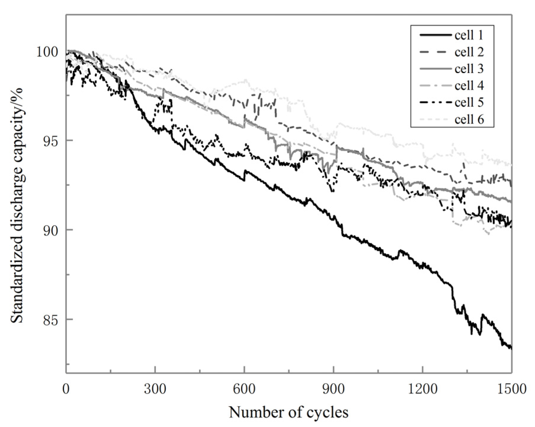
After 1500 cycles of aging experiments, the capacity-fade performance of six cells is obtained, as shown in Figure 3. Experimental results show that the capacity degradation curves of cells under thermal gradient conditions have a high degree of nonlinearity. As can be seen from the figure, cells with thermal gradients demonstrate a slower degradation than the cell without a thermal gradient. The main reason for this phenomenon is that the cell under a thermal gradient performed as a cell at a higher temperature than its theoretical average temperature of the imposed gradient [7]. Such cells can therefore be regarded as cells at elevated temperature, decaying more slowly than cells at room temperature because of a decrease in the ionic conductivity of electrolyte, as well as a slowdown in electrochemical reactions in these cells [16].

3. Proposed Prediction Model

3.1. Extreme Learning Machine

The extreme learning machine is an algorithm for solving single-hidden-layer feedforward neural networks. It has a good learning fitting ability for highly nonlinear, highly nonstationary, and strongly time-varying data, which are widely used in regression prediction. Compared with a traditional neural network algorithm, the ELM model has high accuracy and obvious advantages in learning speed. Its network model is shown in Figure 4.

In Figure 4, x₁~x_n are the inputs of ELM, ω₁₁~ω_nk are the weights between the input layer and the hidden layer, g(x) is the activation function, b₁~b_k are the hidden layer node bias, β₁₁~β_nk are the weights between the hidden layer and the output layer, and y₁~y_n are the outputs of the model.

There are N arbitrary training samples ${\left\{\left(x_i,y_i\right)\right\}}_{i=1}^N$. The n-dimensional input data of the training set in the sample is set as x_i = [x_i1, x_i2, x_i3,···, x_in]^T∈ Rⁿ, and the m-dimensional output value of the training set is set as t_i = [t_i1, t_i2, t_i3,···, t_im]^T∈ R^m. The ELM network model with the number of K hidden-layer nodes and the activation function g_i(x_i) can be represented as:

$${\mathbf{y}}_j={\displaystyle \sum _{i=1}^K{\mathsf{\beta }}_i{g}_i\left({\mathsf{\omega }}_i\cdot {\mathit{x}}_j+{\mathit{b}}_i\right),j=1,2,\cdots ,K}$$

(1)

where ω_i is the input weight vector between the input layer node and the ith hidden layer node; β_i represents the output weight vector connected between the ith hidden layer and the output layer; b_i is the bias of the ith hidden layer node; y_i is the true output of the neural network model; g_i(ω_i∙x_j + b_i) is the activation function.

If there are K hidden-layer nodes, the feedforward neural network can approach any N training samples without errors, and the expression is:

$${\displaystyle \sum _{i=1}^N‖{\mathit{y}}_i-{\mathit{t}}_i‖}=0$$

(2)

That is, the existence of ω_i, β_i, b_i makes:

$${\mathit{t}}_j={\displaystyle \sum _{i=1}^K{\mathsf{\beta }}_i{g}_i\left({\mathsf{\omega }}_i\cdot {\mathit{x}}_j+{\mathit{b}}_i\right)},j=1,2,\cdots ,N$$

(3)

The matrix can be represented as:

$$\mathit{H}\mathsf{\beta }=\mathit{T}$$

(4)

$$\mathit{H}={\left[\begin{array}{ccc}{g}_1\left({\mathsf{\omega }}_1\cdot {\mathit{x}}_1+{\mathit{b}}_1\right)& \cdots & g_i\left({\mathsf{\omega }}_K\cdot {\mathit{x}}_1+{\mathit{b}}_K\right)\\ ⋮& \ddots & ⋮\\ g_i\left({\mathsf{\omega }}_1\cdot {\mathit{x}}_N+{\mathit{b}}_1\right)& \cdots & g_i\left({\mathsf{\omega }}_K\cdot {\mathit{x}}_N+{\mathit{b}}_K\right)\end{array}\right]}_{N\times K}$$

(5)

where H represents the output matrix of the hidden layer; T represents the ideal output vector.

In the ELM algorithm, the input weight vector ω_i and the hidden-layer bias b_i are randomly determined. The output matrix of the hidden layer can be obtained through network training, and the output weight vector β_i is then determined. Equation (4) can be regarded as the least square solution of linear regression based on the generalized inverse theory of matrices, thus obtaining:

$$\widehat{\mathsf{\beta }}={\mathit{H}}^{+}\mathit{T}$$

(6)

where H⁺ is the augmented inverse matrix of matrix H. The reason why the ELM prediction model has a fast learning speed is that ω and b are randomly generated by the network before training. It is only necessary to determine the number of hidden-layer nodes and the corresponding activation function g(x) to obtain the value of the β. The ELM training step is actually to find the linear regression least squares solution, and the optimal solution can be obtained by running it once.

3.2. Sparrow Search Algorithm

The sparrow search algorithm is a swarm intelligence optimization algorithm proposed by Xue et al. [17] in 2020. The algorithm is novel and effective for optimization. The algorithm is inspired by the predatory behavior of sparrow populations, whose rules can be summarized as follows:

(1)

Explorers have higher energy reserve capabilities and provide foraging directions and areas for followers in the population. The health status of an individual determines its energy reserve level.

(2)

When a sparrow perceives a predator, it chirps to tell other sparrows that danger is coming. When the danger level is above the threshold, the explorer guides the sparrows in following it to areas away from the predator.

(3)

Sparrows become explorers on the premise of finding a better food source, but the ratio of explorers to followers remains constant across the population.

(4)

Sparrows with higher energy will become explorers. Many hungry followers will fly to other places to get food, hoping to gain enough energy to become explorers.

(5)

Because the explorer has a good food source, followers will follow the explorer to find food. Meanwhile, to gain energy, followers may spy on the explorer and snatch food when the time is right.

(6)

When perceiving danger, sparrows at the edge of the group will immediately move away from the predator, while those in the middle of the group will fly closer to other sparrows and move around at will.

In the SSA model, the priority of explorers for getting food depends on their fitness. Because of their responsibility for finding food, explorers can fly to a wider area to find food. According to the first two rules of the SSA, the explorer position in the iteration is updated as follows:

$$X_{i,j}^{t+1}=\left\{\begin{array}{c}{X}_{i,j}^t\cdot \exp \left(\frac{-i}{\alpha \cdot ite{r}_{\max }}\right)\begin{array}{cc}& R_2<ST\end{array}\\ X_{i,j}^t+Q\cdot L\begin{array}{cc}\begin{array}{cc}& \end{array}& R_2\ge ST\end{array}\end{array}\right.$$

(7)

where t is the number of real-time iterations, j is the real-time dimension. $X_{i,j}^t$ is the position of the ith sparrow in the jth dimension of the iteration. iter_max is the maximum number of iterations. α is taken randomly from [0, 1]. R₂∈[0, 1] and ST∈[0.5, 1] are hazard values and safety thresholds, respectively. Q is a random number that follows a normal distribution. L is the unit vector where the d-dimensional elements are all 1, and dimension d is the dimension of the variable to be optimized.

When R₂ < ST, indicating that the situation is currently safe, the explorer will look for food in a larger area; when R₂ ≥ ST, it means that the predator is nearby and found by the sparrow, and the group needs to fly quickly to safety. Followers need to implement Rules (4) and (5). Followers frequently spy on the explorer. If they perceive that the explorer has found a high-quality food source, they will immediately fly to its position and fight with it. If the followers win, the explorer’s food belongs to them; if the followers fail, proceed to Rule (5). The position of followers is updated iteratively as follows:

$$X_{i,j}^{t+1}=\left\{\begin{array}{c}Q\cdot \exp \left(\frac{X_{worst}^t-X_{i,j}^t}{i^2}\right)\begin{array}{cc}& i>\frac{n}{2}\end{array}\\ X_P^{t+1}+\left|X_{i,j}^t-X_P^{t+1}\right|\cdot A^{+}\cdot L\begin{array}{cc}& i\le \frac{n}{2}\end{array}\end{array}\right.$$

(8)

where $X_{worst}^t$ represents the worst position of the sparrow population in the tth iteration; $X_P^{t+1}$ represents the best position of the explorer at the t + 1 iteration; A is a 1× d-dimensional matrix with the same input dimensions, and each element in the matrix is randomly 1 or −1; n is the number of sparrows.

When I > n/2, it means that the ith follower has a high probability of being eliminated because of its poor health; when i $\le$ n/2, it represents the update position of the followers in the iteration.

Sparrows that could detect the approach of predators account for 10% to 20% of the total population, and their positions will appear randomly in the sparrow population at the beginning of the algorithm. Rule (6) is expressed as follows:

$$X_{i,j}^{t+1}=\left\{\begin{array}{c}{X}_{best}^t+\lambda \cdot \left|X_{i,j}^t-X_{best}^t\right|\begin{array}{cc}& f_i>f_g\end{array}\\ X_{i,j}^t+J\left(\frac{X_{i,j}^t-X_{worst}^t}{\left(f_i-f_w\right)+\epsilon }\right)\begin{array}{cc}& f_i=f_g\end{array}\end{array}\right.$$

(9)

where $X_{best}^t$ is the global best position for the tth iteration; λ is a random number that represents the step size control parameter and follows a normal distribution with a variance of 1 and a mean of 0; J∈[0, 1] is a random number; f_i is the fitness value of the sparrow; f_g and f_w are the global best fit and the worst fit, respectively; ε is a small constant to avoid f_i − f_w = 0.

To reduce model complexity, when f_i > f_g, Equation (9) represents the latest position of the sparrow at the edge of the group in the iteration. When f_i = f_g, it means that the sparrow in the middle of the population detects an approaching predator and needs to fly to other sparrows. J is the control coefficient of sparrow step length. The flow of SSA is as follows:

Step 1: set algorithm parameters, such as the total number of sparrow population, the number of explorers, the number of sparrows found to be close to the predator, the maximum number of iterations iter_max, and the safety threshold R₂.

Step 2: the algorithm uses mean squared error (MSE) as a fitness function to calculate the health status of sparrows, from which the best and worst fitness values are found.

Step 3: calculate the latest position of the explorer, follower, and sparrow that detects an approaching predator using Equations (7)–(9), respectively. If the sparrow can get more food at this position, the position information is updated.

Step 4: repeat Step 3 and stop iteration when the number of iterations reaches the maximum. The sparrow with the lowest fitness value among all iterations is the optimal solution.

3.3. SSA-ELM Prediction Model

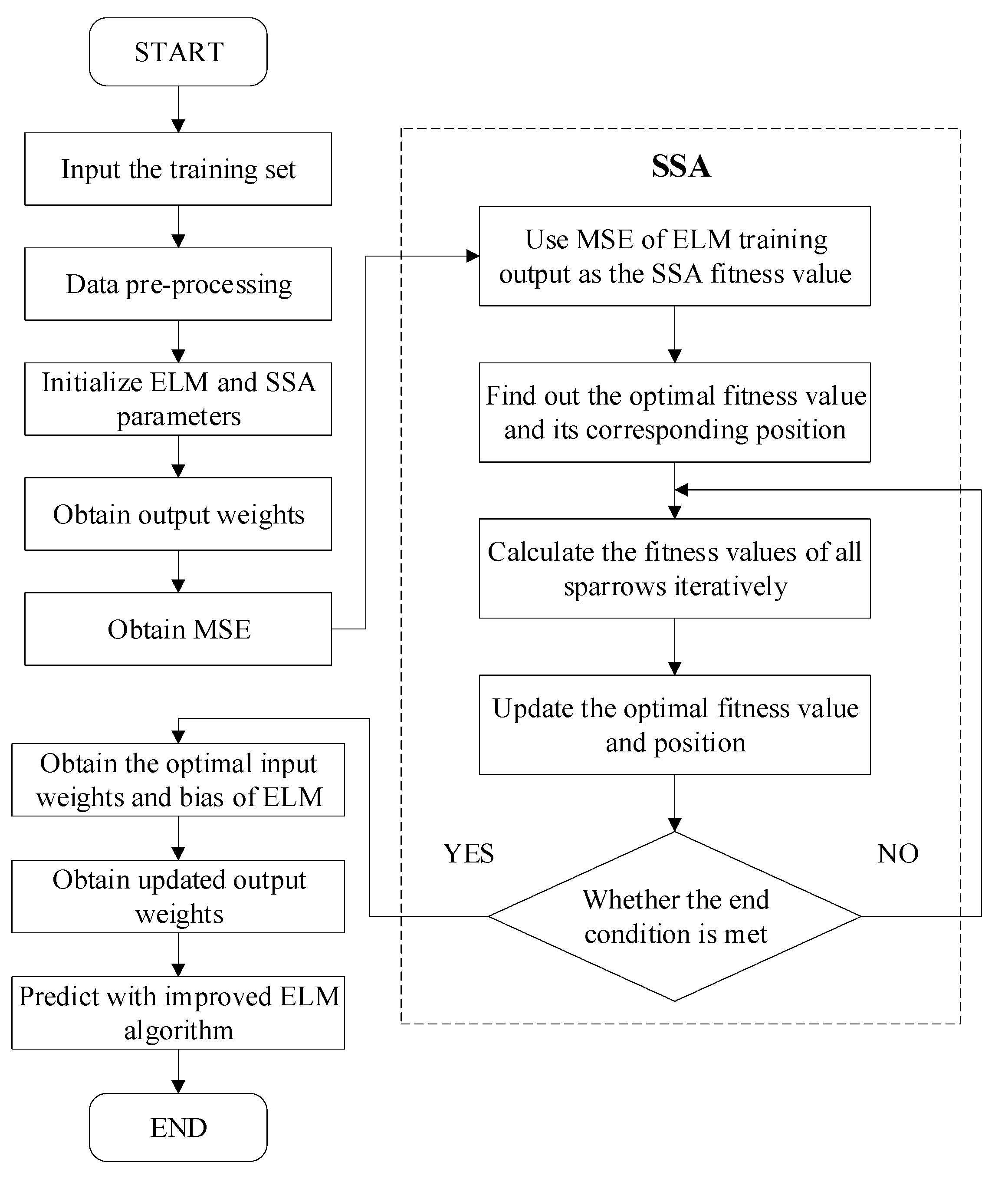
When ELM is used for prediction, the input weights and bias generated by the network model at the initial moment have a greater impact on the model training results because of their randomness. To avoid blind training of the ELM model, this paper uses SSA to optimize input weights and bias of the ELM model. The optimal network weights and bias found by SSA are substituted into the ELM model. The updated output weights and optimized ELM model are obtained and established. The specific algorithm flow of the proposed SSA-ELM hybrid prediction model is shown in Figure 5.

The process of SSA to find the optimal input weights and bias is as follows. Based on the six proposed rules, the SSA first divides the sparrows into explorers, followers, and sparrows that detect an approaching predator. The fitness value of each individual sparrow, MSE, is then calculated. The optimal fitness and the corresponding sparrow position can be therefore obtained. The model is then iterated to find the optimal network weights and bias by comparing the values of the fitness function. In each iteration, the minimum MSE in this iteration is compared with the optimal fitness in all previous iterations. If it is less than the optimal fitness, it indicates this sparrow has better fitness. The optimal position is then updated to that of this sparrow. If it is greater than the optimal fitness, it is not necessary to update the data and proceed directly to the next iteration until the maximum number of iterations is reached. When all iterations are completed, the optimal input weights and bias obtained by SSA are used to build a new ELM prediction model.

4. Results and Discussion

Based on the 1500 cycles aging experiment data of six cells, the accuracy of different algorithms is tested on the platform of Matlab. In the training set, discharge capacity data of the first 800 cycles of six cells are used as model input and discharge capacity of the last 700 cycles of six cells are served as model output.

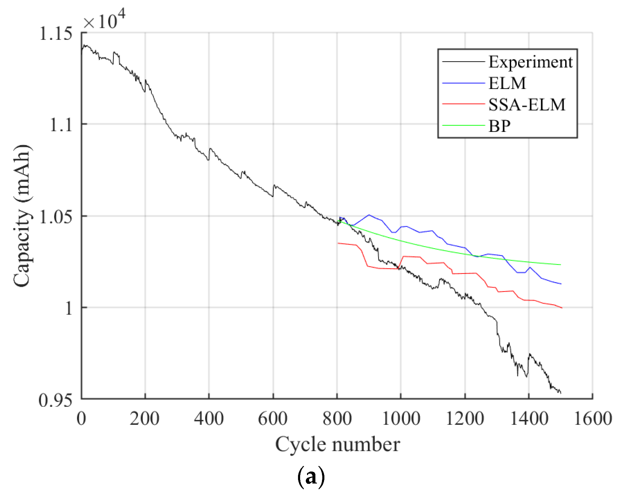
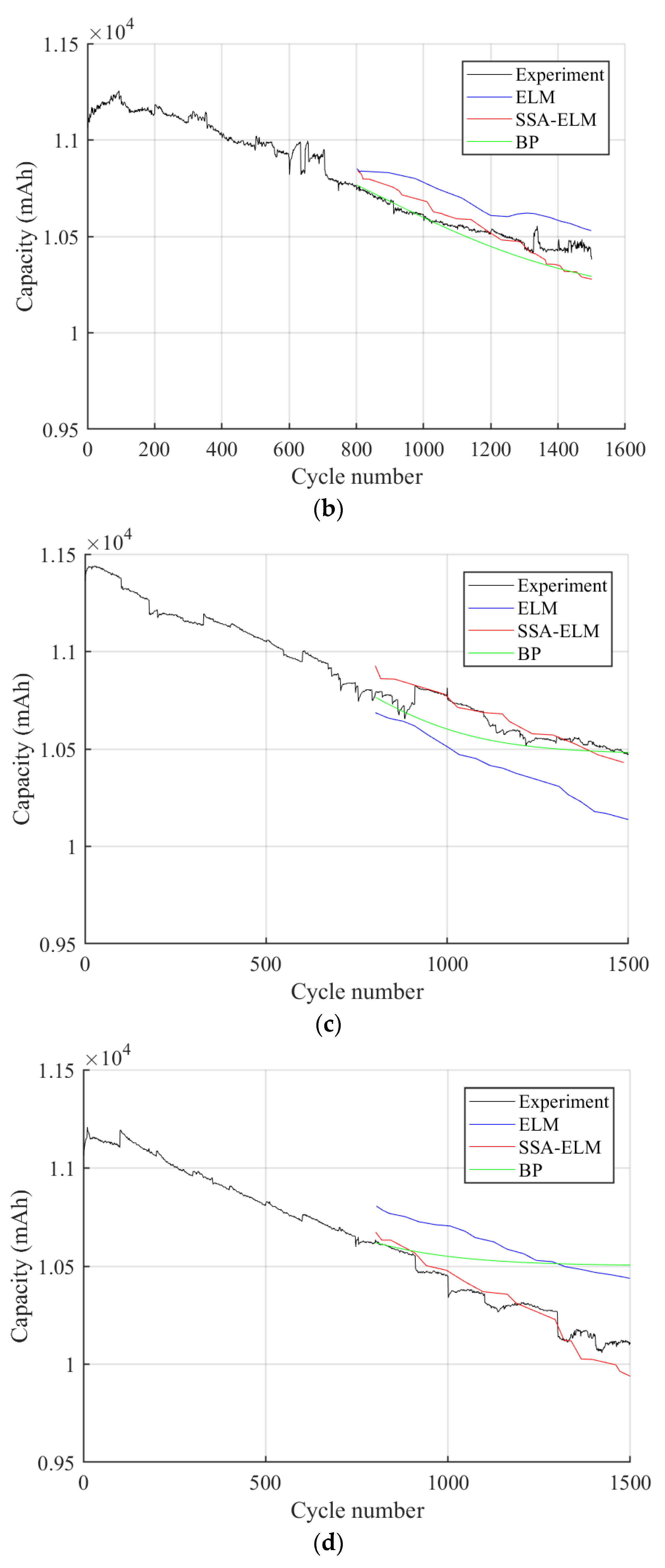
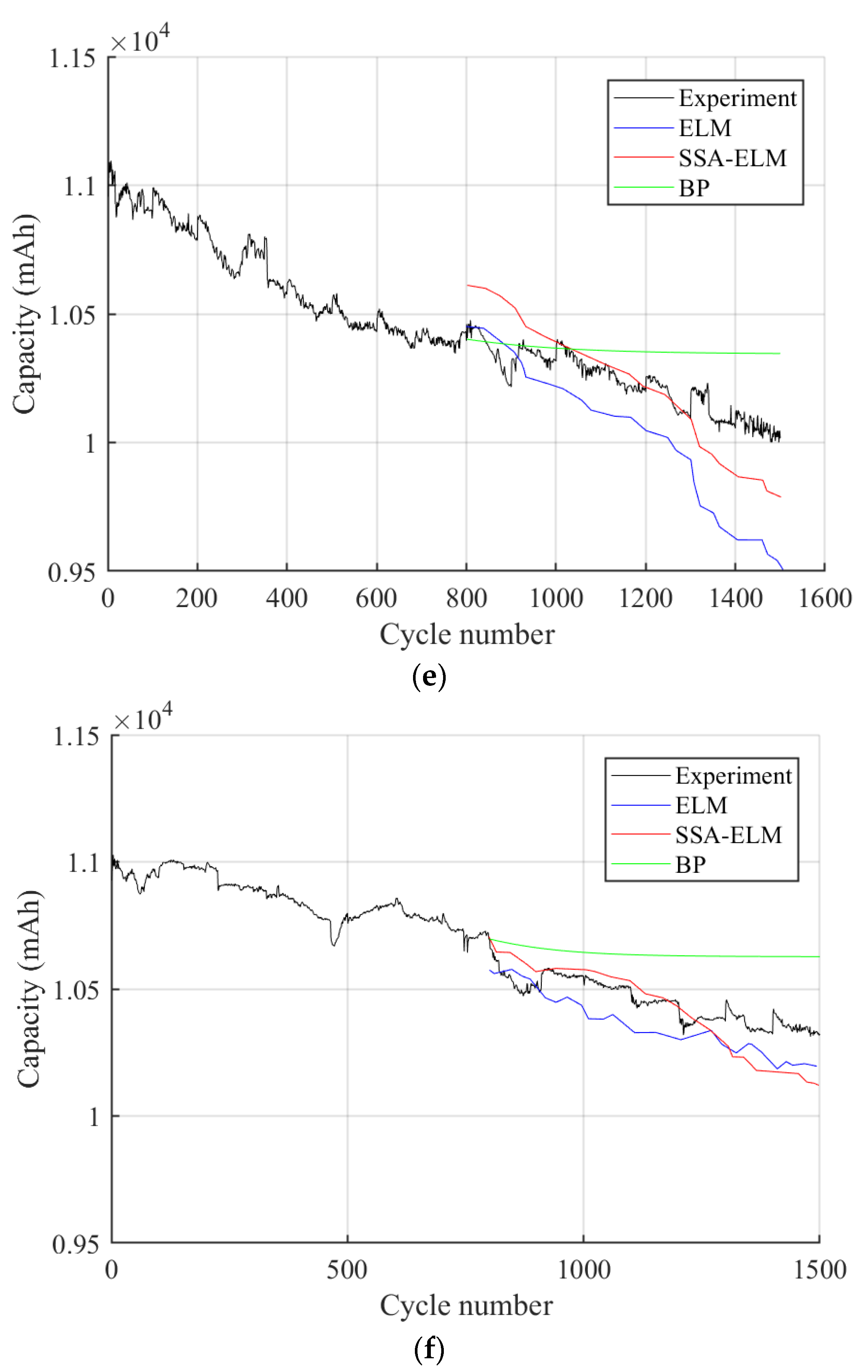
To verify the superiority of the proposed SSA-ELM model for predicting battery life under thermal gradient conditions, the prediction results of six cells are compared with those of the traditional ELM model and back-propagation (BP) neural network, as shown in Figure 6.

The simulation is run in Windows 11 with Intel(R) Core(TM) i7-10700F CPU @ 2.90 GHz, 16.0 GB RAM. The computational time for ELM, SSA-ELM, and BP is about 0.235 s, 138.818 s, and 0.273 s, respectively. By observing Figure 6, it can be intuitively found that the SSA-ELM hybrid prediction model has less fluctuation than the traditional ELM prediction curve and the BP neural network prediction curve. The prediction results of the proposed prediction model have a higher degree of fit with the true value curve.

To increase the reliability of the simulation results, the mean absolute percentage error (MAPE) and root mean square error (RMSE) are added as evaluation indicators of model accuracy. The equations to calculate MAPE and RMSE are as follows:

$$\mathrm{MAPE}=\frac{1}{m}{\displaystyle \sum _{t=1}^m\left|\frac{e_t}{R_t}\right|}$$

(10)

$$\mathrm{RMSE}=\sqrt{\frac{1}{m}{\displaystyle \sum _{t=1}^m{\left(e_t\right)}^2}}$$

(11)

where m represents the prediction time point, e_t represents the absolute error between the actual value at time t and the predicted value, and R_t represents the actual value at time t.

The MAPE and RMSE error indexes of the predicted results of the SSA-ELM model for six batteries were compared with those of the ELM model and BP neural network, as shown in

Table 3. Comparison of prediction results.

Battery Number	MAPE			RMSE (mAh)
	ELM	SSA-ELM	BP	ELM	SSA-ELM	BP
Battery 1	2.9639%	1.8129%	2.8011%	334.63	218.82	342.01
Battery 2	1.3194%	0.6150%	0.5375%	143.62	77.48	72.78
Battery 3	2.1539%	0.4189%	0.6779%	241.02	59.25	90.41
Battery 4	2.7101%	0.5236%	2.0839%	285.52	69.34	250.17
Battery 5	2.1598%	1.1032%	1.3193%	267.29	145.80	165.65
Battery 6	0.9815%	0.7615%	1.8256%	111.91	102.74	203.69
Average value	2.0481%	0.8725%	1.54%	230.67	112.24	187.45

.

As can be seen from the table, most of the MAPE and RMSE of the SSA-ELM prediction result of each battery are lower than that of the ELM and BP. The average value of MAPE of the six cells using the SSA-ELM model is 0.87%, which is lower than that of the ELM and BP. The average value of RMSE is 112.24 mAh, which is also lower than that of the ELM and BP. For batteries 2–6 with different thermal gradients, the SSA-ELM still achieves high accuracy prediction results. This shows that the proposed algorithm has an advantage in predicting data with a high degree of nonlinearity.

According to the results of the algorithm, it is concluded that: (1) compared with the traditional ELM model and BP neural network, the SSA-ELM-based life prediction model has higher prediction accuracy under thermal gradient conditions; (2) the SSA-ELM prediction model can better handle data with high nonlinearity (such as battery capacity degradation data under thermal gradients); and (3) since SSA optimizes the ELM network weights and bias, the proposed prediction model can maintain good prediction stability.

5. Conclusions

Analysis of battery aging experimental data under thermal gradient conditions shows that the capacity degradation curves of lithium batteries under thermal gradient conditions have a high degree of nonlinearity. In this paper, an SSA-ELM model is proposed to improve the robustness of the ELM and the accuracy of RUL prediction. SSA is used to optimize the network weights and bias of the ELM. The life of lithium-ion batteries is predicted based on aging experimental data and the proposed prediction model. Comparing the proposed SSA-ELM prediction model with the traditional ELM and BP neural network, it is found that the average value of MAPE and RMSE of the six cells of SSA-ELM are both lower than those of the ELM and BP, indicating that the SSA-ELM prediction model has higher accuracy. For batteries 2–6 with thermal gradients, the accuracy of the SSA-ELM prediction is highly improved, indicating that the proposed algorithm has an advantage in predicting data with a high degree of nonlinearity.

References

1. Chen, W.; Liang, J.; Yang, Z.; Li, G. A review of lithium-ion battery for electric vehicle applications and beyond. Energy Procedia 2019, 158, 4363–4368. [Google Scholar] [CrossRef]
2. Reddy, R.C.K.; Lin, J.; Chen, Y.; Zeng, C.; Lin, X.; Cai, Y.; Su, C.Y. Progress of nanostructured metal oxides derived from metal–organic frameworks as anode materials for lithium–ion batteries. Coord. Chem. Rev. 2020, 420, 213434. [Google Scholar] [CrossRef]
3. Reddy, R.; Lin, X.; Zeb, A.; Su, C.Y. Metal–Organic Frameworks and Their Derivatives as Cathodes for Lithium-Ion Battery Applications: A Review. Electrochem. Energy Rev. 2022, 5, 312–347. [Google Scholar] [CrossRef]
4. Han, X.; Lu, L.; Zheng, Y.; Feng, X.; Li, Z.; Li, J.; Ouyang, M. A review on the key issues of the lithium ion battery degradation among the whole life cycle. ETransportation 2019, 1, 100005. [Google Scholar] [CrossRef]
5. Liu, J.; Duan, Q.; Qi, K.; Liu, Y.; Sun, J.; Wang, Z.; Wang, Q. Capacity fading mechanisms and state of health prediction of commercial lithium-ion battery in total lifespan. J. Energy Storage 2022, 46, 103910. [Google Scholar] [CrossRef]
6. Hu, Y.; Choe, S.Y.; Garrick, T.R. Measurement of heat generation rate and heat sources of pouch type Li-ion cells. Appl. Therm. Eng. 2021, 189, 116709. [Google Scholar] [CrossRef]
7. Troxler, Y.; Wu, B.; Marinescu, M.; Yufit, V.; Patel, Y.; Marquis, A.J.; Brandon, N.P.; Offer, G.J. The effect of thermal gradients on the performance of lithium-ion batteries. J. Power Sources 2014, 247, 1018–1025. [Google Scholar] [CrossRef]
8. Hu, Y.; Choe, S.Y.; Garrick, T.R. Measurement of two-dimensional heat generation rate of pouch type lithium-ion battery using a multifunctional calorimeter. J. Power Sources 2022, 532, 231350. [Google Scholar] [CrossRef]
9. Liu, X.; Ai, W.; Marlow, M.N.; Patel, Y.; Wu, B. The effect of cell-to-cell variations and thermal gradients on the performance and degradation of lithium-ion battery packs. Appl. Energy 2019, 248, 489–499. [Google Scholar] [CrossRef]
10. Werner, D.; Paarmann, S.; Wiebelt, A.; Wetzel, T. Inhomogeneous temperature distribution affecting the cyclic aging of Li-ion cells. Part I: Experimental investigation. Batteries 2020, 6, 13. [Google Scholar] [CrossRef]
11. Liu, D.; Luo, Y.; Liu, J.; Peng, Y.; Guo, L.; Pecht, M. Lithium-ion battery remaining useful life estimation based on fusion nonlinear degradation AR model and RPF algorithm. Neural Comput. Appl. 2014, 25, 557–572. [Google Scholar] [CrossRef]
12. Hosen, M.S.; Youssef, R.; Kalogiannis, T.; Van Mierlo, J.; Berecibar, M. Battery cycle life study through relaxation and forecasting the lifetime via machine learning. J. Energy Storage 2021, 40, 102726. [Google Scholar] [CrossRef]
13. Deng, Y.; Ying, H.; Jiaqiang, E.; Zhu, H.; Wei, K.; Chen, J.; Zhang, F.; Liao, G. Feature parameter extraction and intelligent estimation of the State-of-Health of lithium-ion batteries. Energy 2019, 176, 91–102. [Google Scholar] [CrossRef]
14. Long, B.; Li, X.; Gao, X.; Liu, Z. Prognostics comparison of lithium-ion battery based on the shallow and deep neural networks model. Energies 2019, 12, 3271. [Google Scholar] [CrossRef] [Green Version]
15. Ng SS, Y.; Xing, Y.; Tsui, K.L. A naive Bayes model for robust remaining useful life prediction of lithium-ion battery. Appl. Energy 2014, 118, 114–123. [Google Scholar]
16. Cao, W.; Li, J.; Wu, Z. Cycle-life and degradation mechanism of LiFePO4-based lithium-ion batteries at room and elevated temperatures. Ionics 2016, 22, 1791–1799. [Google Scholar] [CrossRef]
17. Xue, J.; Shen, B. A novel swarm intelligence optimization approach: Sparrow search algorithm. Syst. Sci. Control Eng. 2020, 8, 22–34. [Google Scholar] [CrossRef]
Figure 1. Block diagram of battery module with forced thermal gradient.
Energies 16 00767 g001
Figure 2. Battery aging test bench under thermal gradient conditions.
Energies 16 00767 g002
Figure 3. Capacity-fade performance of six cells.
Energies 16 00767 g003
Figure 4. Extreme learning machine network model.
Energies 16 00767 g004
Figure 5. SSA-ELM algorithm flow chart.
Energies 16 00767 g005
Figure 6. Comparison of prediction results of six cells. (a) Comparison of the prediction results of battery 1. (b) Comparison of the prediction results of battery 2. (c) Comparison of the prediction results of battery 3. (d) Comparison of the prediction results of battery 4. (e) Comparison of the prediction results of battery 5. (f) Comparison of the prediction results of battery 6.
Energies 16 00767 g006aEnergies 16 00767 g006bEnergies 16 00767 g006c