Prognosis of Lithium-Ion Batteries’ Remaining Useful Life Based on a Sequence-to-Sequence Model with Variational Mode Decomposition

Abstract

The time-varying, dynamic, nonlinear, and other characteristics of lithium-ion batteries, as well as the capacity regeneration phenomenon, leads to the low accuracy of the traditional deep learning models in predicting the remaining useful life of lithium-ion batteries. This paper established a sequence-to-sequence model for remaining useful life prediction by combining the variational modal decomposition with bi-directional long short-term memory and Bayesian hyperparametric optimization. First, variational modal decomposition is used for noise reduction processing to maximize the retention of the original information of capacity degradation. Second, the capacity declining trend after noise reduction is modeled and predicted by the combination of bi-directional long-short term memory and temporal attention mechanism. In addition, a Bayesian optimizer is used to adaptively adjust the hyperparameters while training the model. Finally, the model was validated on NASA and CALCE data sets, and the results show that the model can accurately predict the future trend with only the initial 12% capacity data.

1. Introduction

Lithium-ion batteries have the advantages of high energy density, long cycle life, safety, and reliability. They are widely used in mobile electronic equipment, medical equipment, transportation, power grid energy storage systems, and other fields, and are also gradually being extended to military communications, aerospace, and other fields [1,2,3,4]. Battery health prediction is an important part of the battery management system (BMS). Accurate prediction of battery state of health (SOH) and remaining useful life (RUL) [5] are of key significance to the battery and the whole system.

At present, the common lithium battery RUL prognosis methods include model-based methods and data-driven based methods [6,7,8]. Based on certain empirical knowledge and physical or chemical knowledge, the model-based methods explicitly express the battery capacity decay with a formula, and then recurses the battery aging trajectory to obtain the RUL [9]. Model-based methods can be built through electrochemical models, equivalent circuit models, and empirical models [10,11,12]. Since electrochemical models are difficult to execute on BMS with limited computing resources, and equivalent circuit models are dependent on the impedance data, exponential and power function battery degradation models have been widely used [13]. Sarasketa established a battery degradation model with discharge current, discharge depth, and battery accumulated ampere hours as independent variables, including exponential function and power function [14]. The RUL can be calculated based on the battery degradation model, but the application range of the degradation model determined according to the experiment is limited. For expanding the application range of the model, the filter algorithm is applied to real-time update the model parameters to improve the accuracy of RUL prediction. Particle filters (PF) can be used to estimate the state of nonlinear and non-gaussian stochastic systems. A large number of scholars use PFs to update the parameters of battery degradation models to predict the RUL [15]. He et al. established a battery degradation model with double exponential functions, initialized and updated the model parameters with the Dempster-Shafer theory, and the Bayesian Monte Carlo method, respectively, then predicted the battery RUL [16]. Guha et al. fused the internal resistance (IR) and capacity to obtain a battery decay model, updated the parameters with PF, and predicted the battery RUL [17]. To solve the problem of particle degeneracy, Yang et al. [11] proposed an integrated lithium-ion battery RUL prediction method based on a particle resampling strategy. However, these empirical models are only approximate estimates of battery degradation trajectories, resulting in large RUL prediction errors. Furthermore, the Unscented Kalman Filter (UKF) is suitable for working when the observation noise variance is small, and the PF is influenced by the particle degeneracy issue.

Compared with the model-based methods, the data-driven methods do not rely on accurate battery models, but need to extract the key features from the massive historical data through a specific learning algorithm. It has been widely applied in the health state estimation and RUL prediction of lithium-ion batteries. Data-driven methods include machine learning and deep learning methods. Machine learning is the most recognized data-driven method that has a significant focus on support vector machines (SVM), relevance vector machines (RVM) [18], support vector regression (SVR) [19], and decision tree [20,21], widely used in RUL prediction of lithium-ion batteries. Razavi Far and Pattipati used an extreme learning machine (ELM) and SVM to forcast RUL of lithium-ion batteries [22]. Since capacity shows different decay laws at different stages, Patil et al. applied SVM to predict RUL at the later stage of battery capacity decline [23]. The decline data of similar batteries has a certain guiding significance for RUL prediction, thus Richardson et al. combined multiple battery decline data with GPR to predict RUL to improve prediction accuracy [24]. Although these machine learning tools are widely used and can be explained, they have the following disadvantages: high computing costs (such as GPR and RVM), lack of sparsity (such as GPR and SVM), and lack of stability (such as RVM) for large datasets. Generally speaking, machine learning tools are invalid in the case of large datasets, whether parametric or nonparametric models are used, because they need to be retrained using the entire dataset after adding newly observed data. In addition, most previous studies on machine learning based RUL estimation reported satisfactory performance only under restricted environmental conditions, such as complete cycles under constant current, which does not represent a real scenario [25]. In addition, they require manual health indicators as input features. Different types of batteries may be different so they need expert knowledge of battery systems. Moreover, due to degradation data points contributing more or less to the construction of a precise degradation model, the sparse selection of degradation data will lead to a decline in prediction accuracy.

In recent years, with the development of big data technology and cloud platform services, methods based on deep neural networks have been widely concerned. In order to overcome the limitations of traditional data-driven methods, these methods approach high-dimensional nonlinear functions directly from the original data, and obtain high prediction accuracy in solving complex problems [26,27,28,29,30,31,32]. Zhang et al. [26] combined long short-term memory (LSTM) and Monte Carlo simulation to predict the long-term degradation of learning lithium-ion batteries, and the RUL confidence is given. On the above basis, Li et al. [27] proposed adding peephole connections to LSTM to estimate SOH through a many-to-one structure and predict RUL through a one-to-one structure. Kim et al. [28] proposed a method to predict the state of different types of batteries by integrating deep learning and transfer learning, and estimated RUL and SOH by using the prediction uncertainty with variational reasoning. Ding et al. [29] combined wavelet decomposition, a two-dimensional convolution network, and an adaptive multiple error correction method to verify the effectiveness of the method on the public NASA data set. Hong et al. [30] proposed an end-to-end deep learning framework for the swift prediction of lithium-ion battery remaining useful life by considering temporal patterns and cross-data correlations in the raw data. Kim et al. [31] collected impedance-related features from discharge curves, and then put them into the proposed knowledge-infused recurrent neural network with Monte Carlo dropout to improve the estimation accuracy and robustness. Due to traditional methods being incapable of solving nonlinear and negligible capacity fade in early cycles, Yang et al. [32] combined a convolutional neural network and a long short-term memory network to evaluate battery lifetime in the early-cycle stage. Since diverse aging mechanisms, various cycle profiles, and negligible capacity degradation in the early cycling stages pose significant challenges to accurate life prediction, Chen et al. [33] formulated a two-dimensional and one-dimensional parallel hybrid neural network to build a battery lifetime model. To solve the limitations on current numerical prediction strategies, Pang et al. [34] proposed an interval prediction strategy for lithium-ion battery remaining useful life (RUL) based on fuzzy information granulation and linguistic description. In order to improve the increasing amount of training data and avoid a deep network structure, Zhao et al. [35] combined a broad learning system (BLS) algorithm and a long short-term memory neural network (LSTM) to outstandingly predict the lithium-ion battery capacity and RUL. However, when the data volume is small or the data contains noise, recurrent neural networks such as RNN are prone to lead to underfitting. Futhermore, due to the capacity regeneration phenomenon in the battery degradation curve, the prediction ability based on methods such as RNN will become poor or even fail [11].

In conclusion, there are still some problems: (1) the battery capacity data are noisy because of the capacity regeneration or diving phenomenon occurs, which makes the RNN-based methods invalid. (2) At present, the hyperparameters of many models are not adaptive learning, but artificial selection. (3) At present, most methods usually require 40–70% battery aging data, or even other data to generate accurate prediction results. It is still a big challenge to use only a small amount of historical capacity data to predict the trend of future capacity changes.

To solve the above problems, this paper proposes a lithium-ion battery RUL prediction method based on sequence-to-sequence (seq-to-seq) model with variational mode decomposition (VMD). Firstly, the capacity degradation curve is decomposed using the VMD method, which can effectively decompose complex signals into signals of different frequencies. Secondly, by adaptively selecting super parameters to train the model through the Bayesian optimization algorithm, many appropriate sparse neural networks will share their weights with each other to generate a model with high performance. Finally, with the predicted SOH value, a many-to-many Bi-LSTM based RUL prediction neural network model is proposed, and the next stage capacity of lithium-ion battery is estimated. The experimental results on NASA data sets and CALCE data sets show that the lithium-ion battery aging data can truly represent its capacity decay process, and the proposed hybrid model has high accuracy and robustness in the early RUL prediction of lithium-ion batteries. The specific contributions of this study are as follows:

(1)

A hybrid deep learning model named VMD-BiLSTM-Attention is proposed to predict the battery lifetime at an early stage. Only the first 12% of discharging capacity are required to evaluate battery remaining useful life. In other words, the proposed model is capable of accurately predicting the lifetime of one battery before it deteriorates obviously.

(2)

The applied deep learning technique automates hyperparameters selection, avoiding the human-labor-based selection and the risk of missing the best model. The hyperparameters learned by deep learning have a stronger stability to give accurate predictions for new inputs that have never been seen during the training stage.

(3)

In the VMD-BiLSTM-Attention model, the cycle-to-cycle evolution of the discharging process is selected as the input. The VMD and BiLSTM are utilized to eliminate capacity noise and capture temporal information, respectively. The model architecture and implementation setups are demonstrated in detail.

The structure of this paper is as follows: Section 2 introduces the relevant algorithms in this paper; Section 3 introduces the battery data and pretreatment methods in detail, and then the complete experimental process of variable current lithium-ion battery aging data sets and the resulting RUL prediction methods used in this experiment are introduced in detail, and the specific evaluation criteria are given; Section 4 is the conclusion.

2. Methods

2.1. VMD

VMD is an adaptive, completely non-recursive modal transformation and signal processing technology. VMD improves the end effect and modal component localization in empirical mode decomposition (EMD), and has a more solid mathematical basis. For time series with high complexity and strong nonlinearity, it can reduce the nonstationarity of the signal and decompose it to obtain relatively stable subsequences containing multiple different frequency scales, which is very suitable for non-stationary sequence signal extraction. The essence of the variational problem is the maximum value problem of the functional, and its core is to obtain n modal components (t), making the sum of the bandwidth of each mode the minimum, and the sum of the modes is equal to the input signal f. The constrained variational model is as follows.

$$\{\begin{array}{l}\underset{\left\{u_n\right\},\left\{w_n\right\}}{\min }\{{\displaystyle \sum _n\parallel {\partial }_t[(\delta (t)+j/\pi t)\times u_n(t)]e^{-j{w}_{n}t}{\parallel }_2^2}\}\\ s.t.{\displaystyle \sum _n{u}_n=f}\end{array}$$

(1)

where ${\partial }_t$ means partial derivative of t, and $\delta (t)$ means impulse function. The VMD algorithm introduces a quadratic penalty term and a Lagrange multiplication operator. The former can ensure the reconstruction accuracy of signal, and the latter can enhance the effect of constraint conditions. The augmented Lagrange function expression is shown below.

$$L(\{u_n\},\{w_n\},\lambda )=\alpha {\displaystyle \sum _n\parallel {\partial }_t[(\delta (t)+j/\pi t)\times u_n(t)]e^{-j{w}_{n}t}{\parallel }_2^2}+\parallel f(t)-{\displaystyle \sum _n{u}_n(t)}{\parallel }_2^2+\langle \lambda (t),f(t)-{\displaystyle \sum _n{u}_n(t)}\rangle$$

(2)

The solution of the minimum problem in Formula (2) is the saddle point in Formula (3). Here, the alternating direction method of multipliers (ADMM) is used to solve the above variational problem by updating u_n^k+1, w_n^k+1, λ^k+1 to find the saddle point of the augmented Lagrangian function and the Parseval/Plancherel Fourier isometric transformation to convert the frequency domain to obtain modal component u_n.

$${\hat{u}}_n^{k+1}(w)=\frac{\hat{f}(w)-{\displaystyle \sum _{i\ne n}\widehat{u_i}(w)+\frac{\hat{\lambda }(w)}{2}}}{1+2\alpha {(w-w_n)}^2}$$

(3)

Similarly, the updated method of center frequency can be obtained by Formula (4), updated according to the Formula (5), until it converges to meet Formula (6), resulting in getting n modal components.

$$w_n^{k+1}=\frac{{\displaystyle {\int }_0^{\infty }w\mid {\hat{u}}_n(w){\mid }^2}dw}{{\displaystyle {\int }_0^{\infty }\mid {\hat{u}}_n(w){\mid }^2}dw}$$

(4)

$${\hat{\lambda }}^{k+1}(w)={\hat{\lambda }}^k(w)+\tau ({\hat{f}}^k(w)-{\displaystyle \sum _n{\hat{u}}_n^{k+1}}(w))$$

(5)

$${\displaystyle \sum _n\parallel u_n^{k+1}-u_n^k{\parallel }_2^2/\parallel u_n^k{\parallel }_2^2<\epsilon }$$

(6)

2.2. Bi-LSTM

LSTM is no longer an ordinary hidden node, but a storage unit with memory function, which can effectively avoid gradient distortion or explosion after a long time-sequence, and overcome the difficulties encountered in traditional RNN training. The key to LSTM lies in the cell state and various gate structures, including the forgetting gate, input gate, and output gate. The unit state can store historical information and update the information through continuous transmission. Therefore, the unit state can be regarded as the “memory” of the network. The illustrative structure of the LSTM predictor is shown in Figure 1a.

$$i_c^{(t)}=\sigma \left(W_i\cdot \left[h^{(t-1)},x_t\right]+b_i\right)$$

(7)

$$f_c^{(t)}=\sigma \left(W_f\cdot \left[h^{(t-1)},x_t\right]+b_f\right)$$

(8)

$$o_c^{(t)}=\sigma \left(W_o\cdot \left[h^{(t-1)},x_t\right]+b_o\right)$$

(9)

$${\stackrel{\wedge }{s}}_c^{(t)}=tanh(W_C\cdot \left[h^{(t)},x_t\right]+b_C$$

(10)

$$S_c^{(t)}=f_c^{(t)}\times S_c^{(t-1)}+i_c^{(t)}\times {\stackrel{\wedge }{s}}_c^{(t)}$$

(11)

$$h^{(t)}=o_c^{(t)}·tanh\left(S_c^{(t)}\right)$$

(12)

In the above formulas, h and x represent the output samples and input samples of the network, respectively, o, i, and f represent the three gates mentioned above, the matrices W and b indicate the weight parameter and the bias term, respectively, and S represents the cell state. σ(·) is the activation function ReLU. Through the Formulas (7)–(12), the error and weight of each LSTM neuron in the back propagation process to update the network data can be calculated, and thus gradually calculates the output value of the LSTM model. The number of neurons is in direct proportion to the computing power and complexity of the neural network. In addition, because the number of network parameters is determined by the number of neurons in each layer, increasing the number of hidden layers will increase the geometric times of the parameters to be trained, and its complexity is several times that of increasing the number of neurons in a single layer. In order to solve the above problems, a BiLSTM network is proposed to model, which not only avoids the operation of manually adding time frames, but also captures the information of future states. A BiLSTM network is composed of forward and backward LSTM networks. It can not only obtain the past information of input data, but also use future information. It is very helpful for sequence data tasks.

As can be seen from the above Figure 1b, BiLSTM is composed of an output layer, a forward hidden layer, a backward hidden layer, and an output layer. The input layer contains a series of input data. The data of the input layer is input to the forward hidden layer and also input to the backward hidden layer, so as to achieve the purpose of paying attention to the upper and lower sequence information at the same time; the forward hidden layer is the forward flow LSTM from start to end, and the backward hidden layer is the reverse flow LSTM from end to start. The input of the output layer node is composed of the output of the reverse hidden layer and the output of the forward hidden layer, and the final output sequence. In the structure, w1 and w3 are the weights from the input layer to the forward and backward hidden layers, respectively, w2 and w5 are the weights from the hidden layer to the hidden layer itself, and w4 and w6 are the weights from the forward and forward hidden layers to the output layer, respectively. The mathematical expression are as follows:

$${\stackrel{\rightharpoonup }{h}}_t=LSTM(x_t,\stackrel{\rightharpoonup }{h_{t-1}})$$

(13)

$$\overleftarrow{h_t}=LSTM(x_t,\overleftarrow{h_{t-1}})$$

(14)

$$y_t=f(W_{\stackrel{\rightharpoonup }{h}}\stackrel{\rightharpoonup }{h_t}+W_{\overleftarrow{h}}\overleftarrow{h_{t-1}}+b)$$

(15)

The forward hidden layer reads the data in time order, makes the information pass forward along the time starting point, and obtains the previous information of the sequence; the backward hidden layer reversely transmits information to obtain the following information of the sequence. By combining the forward layer and backward layer states at the same time, as the hidden layer state output represents the sequence context information, this structure ensures that the BiLSTM can obtain the past and future information at the same time. There is no information flow between the forward and backward hidden layers. The output of the forward LSTM will only be transmitted to the forward LSTM unit, and the output state of the reverse LSTM will only be transmitted to the reverse LSTM unit, which ensures that the expanded map is noncyclic. Although there is no connection between the two directions of the BiLSTM, because they jointly synthesize the output, the final output state sequence also contains the temporal context information.

2.3. Seq-to-Seq NN Based on VMD-BiLSTM-Attention

A seq-to-seq NN network is proposed for early RUL prediction in this section and the structure is shown in Figure 2. The two datasets are employed for training and testing the VMD-BiLSTM seq-to-seq model. The VMD-BiLSTM-Attention model is optimized by the Adam technique and an adaptive superparameter method. The adaptive superparameter method, based on the Bayesian optimization algorithm, automatically filter out the set of candidate superparameters meeting the learning objective task from the initial space of superparameters. Therefore, the proposed model is less sensitive to abnormal capacity value and deeply understands the degradation trend. Note that the performance of the BiLSTM-Attention neural network is sensitive to the number of neurons and dropout value. The range of neurons and dropout value are set from 10 to 200 and 0 to 0.5, respectively. Thus, the wide search space makes the BiLSTM obtain better accuracy and robustness. Adaptive moment estimation can replace the traditional stochastic gradient descent process. It is a first-order optimization algorithm and updates the neural network weights iteratively based on training data. In addition, an attention mechanism allocates computing resources to more important tasks under the condition of limited computing power. Therefore, the early prediction of degradation patterns for LIBs can be realized based on the proposed model. The entire seq-to-seq model training process is summarized in Algorithm 1.

Algorithm 1. Outline of seq-to-seq RUL prediction model for lithium batteries.
1:	Input: The training set Ltrain
2:	Output: Trained sequence-to-sequence model parameters
3:	Initialize parameters
4:	Repeat
5:	Forward Propagation:
6:	do
7:	Step1: Conduct VMD operation with the capacity data in Equations (1)–(6).
8:	Step2: Use BiLSTM Equations (7)–(15) to predict RUL using the SOH result from VMD.
9:	Step3: Use dropout to prevent overfitting
10:	Step4: Use temporal attention mechanism to focus sequence key in formation
11:	Step5: Use time-distributed fully connected dense layer to handle time dimension of sequence.
12:	Step6: Calculate the MAE introduced in Equation (18) between the prediction and targets.
13:	end
14:	Backward Propagation:
15:	Compute the gradient using Adam and update network parameters
16:	until A predefined small loss

3. Results

3.1. Data Sets Description

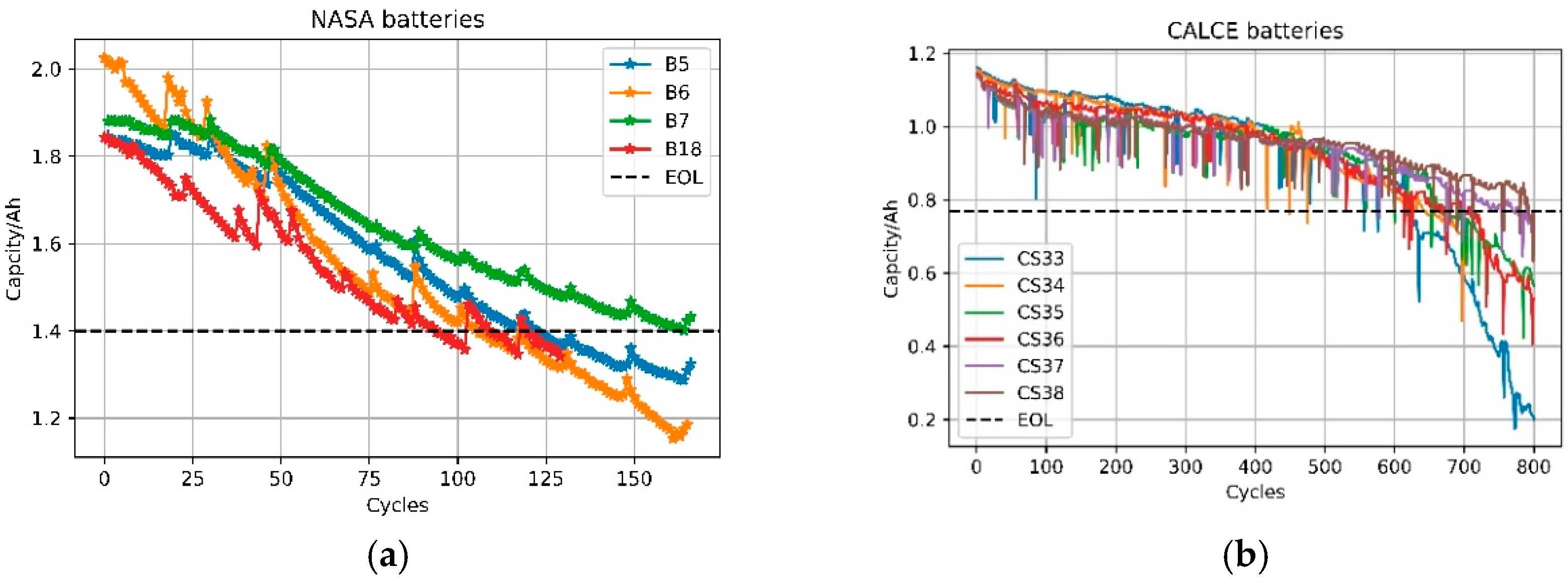
In this paper, the NASA dataset [36] and CALCE dataset [16] are applied to verify the effectiveness of the mentioned framework. The NASA batteries are 18,650 lithium-cobalt batteries with a rated capacity of 2 Ah. The aging experiment of lithium batteries mainly goes through two processes: charging and discharging. The charging process is mainly to charge in the constant current (CC) mode of 1.5 A until the voltage reaches 4.2 v, and then continue to charge in the constant voltage (CV) mode until the current drops to 20 mA. The discharge modes are different. B5, B6, B7, and B18 adopt 1C constant current discharge. Discharge was carried out at a constant current level of 2A until the battery voltage fell to 2.7 v, 2.5 v, 2.2 v, and 2.5 v for batteries B5, B6, B7, and B18, respectively, at room temperature. As shown in Figure 3a, the aging attenuation of different batteries are shown. The lithium battery decays to 70% of the rated capacity in 166 charge and discharge cycles. It is worth noting that the capacity of the lithium battery will increase abruptly in the process of performance degradation because of the relaxation of the physical and chemical reactions of the lithium battery during the rest period, realizing the regeneration of lithium batteries. The CALCE batteries have a graphite anode and a lithium cobalt oxide (LiCoO2) cathode with a rated capacity of 1.1 Ah. All CS2 batteries have gone through the standard constant current/constant voltage protocol. The constant current rate is 0.5 C until the voltage reaches 4.2 V, and then 4.2 V is maintained until the charging current drops below 0.05 A. Unless otherwise specified, the discharge cut-off voltage of these batteries is 2.7 V. The aging curve of CALCE batteries are shown in Figure 3b.

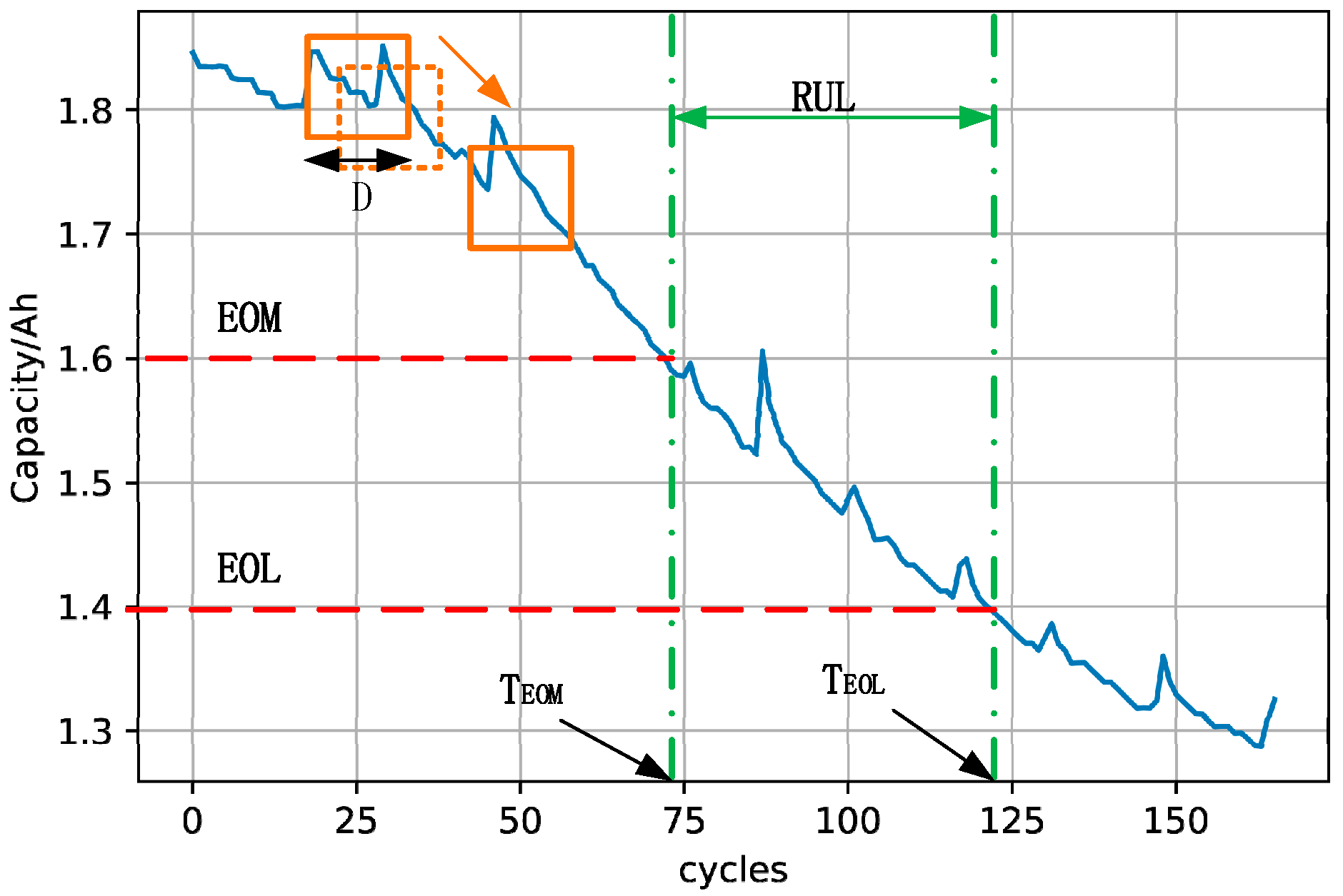
Figure 3 shows the degradation process curves of the discharge capacity of lithium-ion batteries. It can be seen from the graph that the degradation rate of each battery is different due to different discharge depths. With the increase of the cycle period, the degradation capacity of the batteries not only have an obvious downward trend, but also have obvious capacity regeneration phenomenon and random noise interference. The battery state fluctuates frequently, and the degradation data shows significant non-stationarity and non-linearity. Battery RUL is generally defined as the number of charging and discharging cycles that the operating state of the battery decays to the set failure threshold under specific operating conditions, in which the capacity state of the battery is the most commonly used threshold indicator. The starting capacity value used for RUL prediction is called the end of monitoring (EOM), corresponding to the number of cycles T_EOM. The end of life threshold (EOL) is the capacity value at the time of battery failure, corresponding to the number of cycles T_EOL. Therefore, the battery RUL can be specifically defined as:

RUL = 𝑇_EOL – 𝑇_EOM

(16)

The battery RUL prediction process is shown in Figure 4, where D is the predicted sliding window size. According to the existing literature, when the battery cycle capacity decays to 70% of the initial capacity value, it is considered that the battery has reached the end of its life [37]. Therefore, accurate battery capacity prediction is the key to achieve battery remaining life prediction.

3.2. VMD Results

From the capacity degradation curve, it can be seen that there is a lot of noise in the battery data, which is caused by the complex physical and chemical reactions inside the battery and the changes in practical applications, and is extremely unfavorable for the prediction of battery capacity. This problem can be solved by VMD decomposition of the signal, so that more accurate neural network prediction results can be obtained.

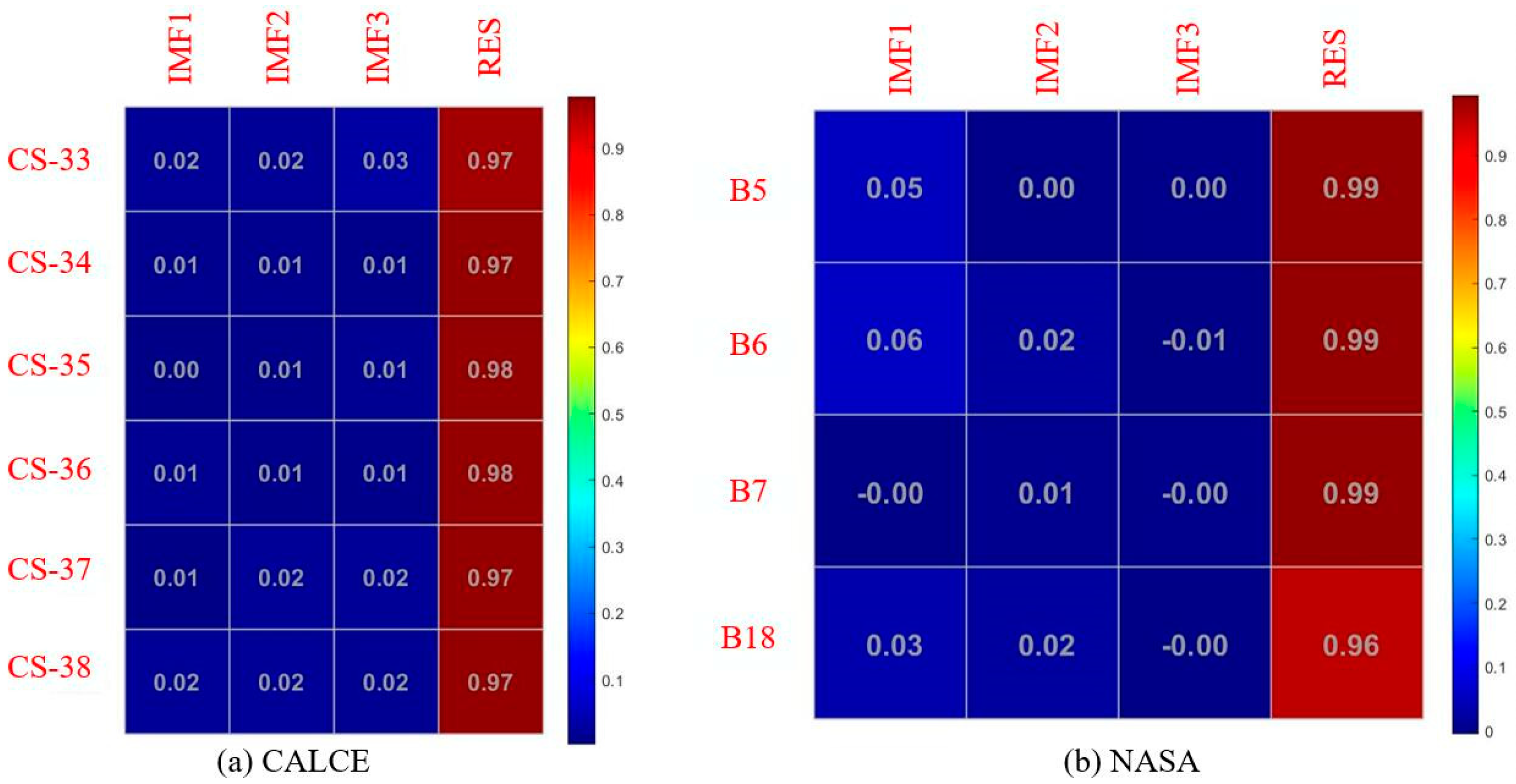
In this paper, the number of modes to be decomposed k is 4, noise-tolerance τ is 0, moderate bandwidth constraint α is 2000, and ε is 1 × 10⁻⁷. Figure 5 shows the original capacity data of the NASA B5 and the curves of the residual (RES) and intrinsic mode functions (IMFs) after the VMD method. Figure 6 shows the original capacity data of the CALCE CS34 and the curves of the RES and IMFs after the VMD method. RES not only maintains the degradation characteristics of the original data, but also is smoother than the original data and effectively eliminates the noise. It is obvious from the VMD separation results in Figure 5 that the capacity fading signal is successfully separated. Although the amplitude of the time domain waveform is different from that of the original signal, it does not affect the result. The separated capacity fading signal is smooth and undistorted. Therefore, if RUL is predicted directly based on the original data, it will be affected by noise fluctuations, which will greatly increase the prediction error. Meanwhile, the prediction of RES is unlikely to cause large errors because of the same trend between RES and the original data. Although the accuracy of prediction may increase for each IMF and the results of integration with RES, many components may increase the calculation time, thus increasing the computational complexity. As shown in Figure 7, in order to analyze the specific relationship between each component after VMD decomposition and the original data, spearman correlation coefficients are calculated. The correlation coefficient between each IMF component and the original value is lower than 0.1, while the correlation coefficient of RES is higher than 0.96. It shows that RES and the original data show a high correlation, and further explains that the prediction of RES changes can truly reflect the capacity degradation.

3.3. Training Detail

This experiment is implemented based on software and hardware such as CPU (Intel Core i7-8700k 3.2 ghz), GPU (NVIDIA geforce GTX 1660ti 6 GB) RAM memory (16 GB), the Windows operating system, and the Keras environment (with TensorFlow as the back end). The sequence-to-sequence model structure used in the experiment consists of an input layer, two BiLSTM layers with attention mechanism, two dropout layers, a full connection layer, and an output layer. After building the seq-to-seq model, it is necessary to determine the loss function for network training to obtain the convolutional neural network parameters. In this experiment, the mean absolute error (MAE) is taken as the loss function, and Adam is used as the adaptive optimizer to minimize the objective function. The learning rate is set to 0.000001, the first-order momentum attenuation coefficient is 0.9, the second-order momentum attenuation coefficient is 0.999, and the batch size is 32. In addition, the number of experimental epoch is set to 300. The sample capacity needs to be normalized before being used in the seq-to-seq neural network. The processing method is as follows:

$$x_{norm}=\frac{x-x_{min}}{x_{max}-x_{min}}$$

(17)

where the lower x_norm is the normalized data, x is the vmd data, x_max is the maximum value in the VMD results, and xmin is the minimum value in the VMD results. The normalized data is in the interval [0, 1]. Meanwhile, in order to quantitatively describe the performance of the lithium-ion battery SOH estimation method, this section uses mean absolute error (MAE), root mean square Error (RMSE), and relative error (RE) as performance evaluation functions, which are respectively:

$$MAE=\frac{1}{N}{\displaystyle \sum _{n=1}^N|c_n-c_n{}^{\prime }|}$$

(18)

$$RMSE=\sqrt{\frac{1}{n}{\displaystyle \sum _{i=1}^n{(c_n-c^{\prime }{}_n)}^2}}$$

(19)

$$RE=\frac{|{\mathrm{RUL}}_{\mathrm{p}}-{\mathrm{RUL}}_{\mathrm{r}}|}{{\mathrm{RUL}}_{\mathrm{r}}}$$

(20)

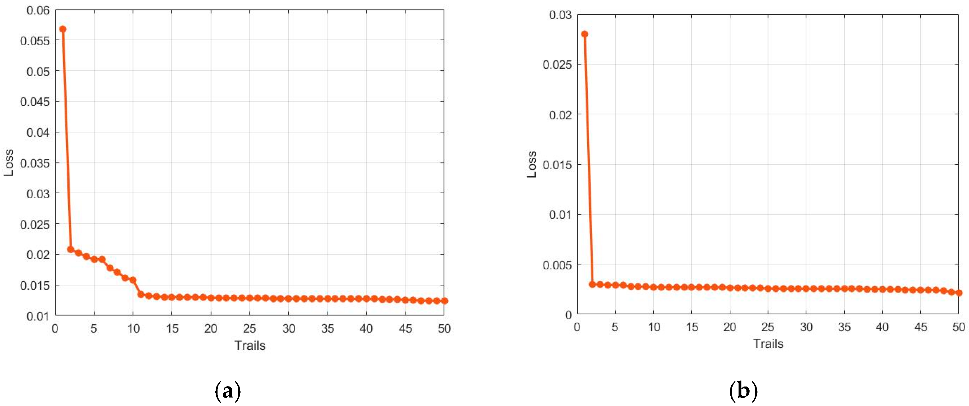
where c_n, c’_n, RUL_r, and RUL_p are true value, predicted value, true RUL, and predicted RUL, respectively. The smaller RMSE, MAE, and RE, the better the prediction performance of the model. In addition, KerasTuner with Bayesian optimization is used to optimize hyperparameters that solve the pain points of the hyperparameter search, which is shown in Figure 8. After 10 times of superparameter optimization, the best superparameter was found in the CACLE dataset, while NASA found the best superparameter after 4 times of searching due to its limited data.

3.4. Results and Discussion

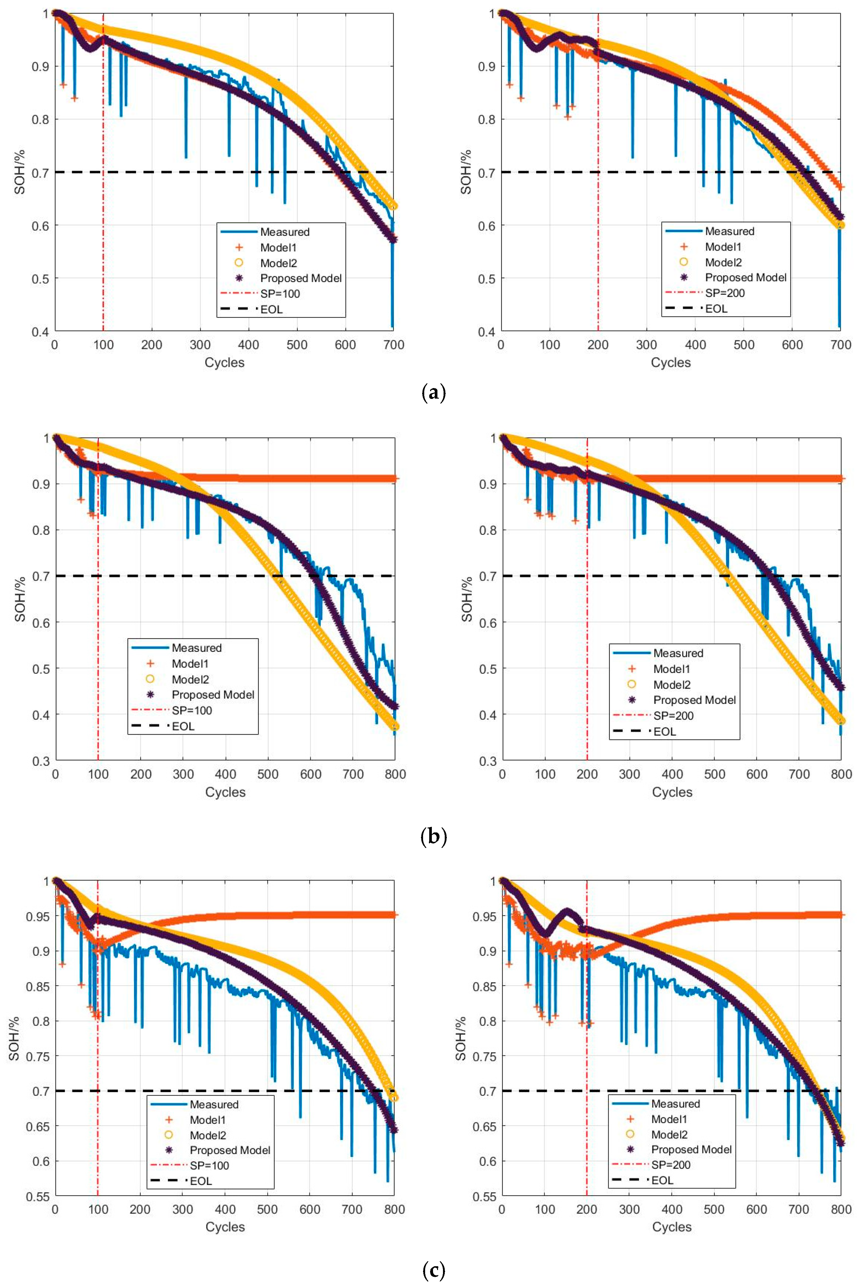
In this paper, when the battery capacity drops to 70% of the nominal capacity, it is the EOL of each battery. The proposed model is validated by the data sets of five cells at different current rates and cut-off voltages. The early recognition result of battery degradation mode based on our method is shown in Figure 9. CS33, CS35, and CS38 are used for training, and CS34, CS36, and CS37 are used for test data. The values of the hyperparameters in the random search shown when the BiLSTM units are from 10 to 200, and step is 10, the dropout = [0.1, 0.2, 0.3, 0.4, 0.5]. Based on the results of the grid search, the final hyperparameters selected were units = 80, dropout = 0.4, window size = [15, 1], and result shape = [5, 1]. After the superparameters are determined by Bayesian optimization, the NN model needs to be fully trained. The capacity data of CS2-33, CS2-35, and CS2-38 are used for RUL model training, and the remaining battery data were used for testing. In addition, three comparison models are defined: model1, model2, and model3. Model1 uses raw data for training. Model2 conducts training based on EMD decomposed data [32], and model3 trains VMD data. We tested the variation trend of RUL derived from 12% and 20%. It can be seen that the three can better characterize the capacity degradation trend, but the accuracy is different. Among them, the prediction after VMD can better fit the degradation trend of the original data and obtain the minimum loss value. However, some RUL predictions trained with the original data cannot even show the degradation trend. The possible reason is that the original data has too much noise and the training model cannot converge well. Figure 10 compares the impact of different sequence lengths on the model and the effect. It compares 10 to 10, 19 to 1, 12 to 8, 14 to 6, and 14 to 6, respectively. Small estimation errors are obtained on the three test batteries, but for the CACLE dataset, the prediction loss of 15 to 5 is the smallest.

Table 1. Performance on the CALCE dataset.

Battery ID	SP	RUL	PRUL	RE/%	RMSE	MAE
CS34	100	602	590	1.9	0.026	0.017
	200	602	621	3.1	0.025	0.015
CS36	100	618	608	1.6	0.048	0.028
	200	618	630	1.9	0.028	0.016
CS37	100	726	746	2.7	0.036	0.029
	200	726	736	1.4	0.034	0.026

shows the different start point (SP) for the CS34, CS36, and CS37 battery. The predicted values of SP = 100 (12%) and SP = 200 (20%) were very close to the real values, indicating that the method could effectively estimate the battery’s RUL at an early stage.

In the NASA data, B5 and B6 are used for testing, while B7 and B18 are used for training. The EOL of each battery is set at the moment that battery declines to 70% of the nominal capacity in the NASA dataset. Figure 11 shows the RUL prediction results of B5 and B6 in the NASA dataset, of which the RUL prediction RE of B5 is 5.6% and 4.0% when starting from 100 and 200, respectively. The prediction error of B6 is 8.2% and 4.5% when the prediction starts from 100 and 200, respectively. For NASA, we can see from the figure that the effect of prediction and regression of the data after emd and vmd is similar, because the noise of the original data itself is not very much. In this way, a simpler emd can achieve good results, and even the emd effect of a battery is better than that of vmd. Such as the prediction of 20% of B5. Figure 10a shows the comparison of prediction results under different sequence lengths. It can be seen from the chart that when the optimal sliding window is selected, NASA’s optimal sequence to sequence is 7 to 3. For B5, when the sequence length is 9 to 1, 8 to 2, 6 to 4, and 5 to 5, it is 0.0122, 0.0120, 0.0126, and 0.0127, respectively. For B6, when the sequence length is 9 to 1, 8 to 2, 6 to 4, and 5 to 5, it is 0.0138, 0.0141, 0.0144, and 0.0146, respectively. If the sliding window is too small or too large, the RUL prediction error will become larger, the performance will be degraded, and even the prediction will become invalid.

Table 2. Performance on the NASA dataset.

Battery ID	SP	RUL	PRUL	RE	RMSE	MAE
B5	20	124	131	5.6	0.026	0.022
	30	124	129	4.0	0.028	0.024
B6	20	109	100	8.2	0.036	0.030
	30	109	104	4.5	0.034	0.026

shows the different start points (SP) for the B5 and B6 batteries. The predicted values of SP = 20 (12%) and SP = 30 (20%) were very close to the real values, indicating that the method could effectively estimate the battery’s RUL at an early stage.

4. Conclusions

As an important object of industrial fault prediction and health management, lithium-ion batteries have a wide range of common problems in industrial RUL prediction, such as nonlinearity and non-stationarity. In this paper, the RUL of the battery is estimated by using a sequence-to-sequence model with variational mode decomposition, providing some reference for the accurate RUL estimation of electric vehicles. The next step is to simplify the model and use high-performance hardware, such as nano, Xavier, and other edge computing devices based on graphics cards to deploy our model to the embedded end, so as to realize SOH estimation and RUL prediction in real vehicles, which will have great prospects.

References

1. Xiong, R.; Li, L.; Tian, J. Towards a smarter battery management system: A critical review on battery state of health monitoring methods. J. Power Sources 2018, 405, 18–29. [Google Scholar] [CrossRef]
2. Ge, M.F.; Liu, Y.; Jiang, X.; Liu, J. A review on state of health estimations and remaining useful life prognostics of lithium-ion batteries. Measurement 2021, 174, 109057. [Google Scholar] [CrossRef]
3. Wang, Y.; Tian, J.; Sun, Z.; Wang, L.; Xu, R.; Li, M.; Chen, Z. A comprehensive review of battery modeling and state estimation approaches for advanced battery management systems. Renew. Sustain. Energy Rev. 2020, 131, 110015. [Google Scholar] [CrossRef]
4. Liu, K.; Wei, Z.; Yang, Z.; Li, K. Mass load prediction for lithium-ion battery electrode clean production: A machine learning approach. J. Clean. Prod. 2021, 289, 125159. [Google Scholar] [CrossRef]
5. Liu, K.; Ashwin, T.R.; Hu, X.; Lucu, M.; Widanage, W.D. An evaluation study of different modelling techniques for calendar ageing prediction of lithium-ion batteries. Renew. Sustain. Energy Rev. 2020, 131, 110017. [Google Scholar] [CrossRef]
6. Takagishi, Y.; Yamaue, T. Prediction of Li-ion Battery Module Performance under Running Condition Based on “Multifactorial Degradation Model”. Int. J. Automot. Eng. 2017, 8, 143–148. [Google Scholar] [CrossRef] [PubMed] [Green Version]
7. Liu, K.; Wei, Z.; Zhang, C.; Shang, Y.; Teodorescu, R.; Han, Q.-L. Towards long lifetime battery: AI-based manufacturing and management. IEEE/CAA J. Autom. Sin. 2022, 9, 1139–1165. [Google Scholar] [CrossRef]
8. Liu, K.; Gao, Y.; Zhu, C.; Li, K.; Fei, M.; Peng, C.; Zhang, X.; Han, Q.-L. Electrochemical modeling and parameterization towards control-oriented management of lithium-ion batteries. Control Eng. Pract. 2022, 124, 105176. [Google Scholar] [CrossRef]
9. Hu, X.; Li, S.; Peng, H. A comparative study of equivalent circuit models for Li-ion batteries. J. Power Sources 2012, 198, 359–367. [Google Scholar] [CrossRef]
10. Wei, J.; Dong, G.; Chen, Z. Remaining useful life prediction and state of health diagnosis for lithium-ion batteries using particle filter and support vector regression. IEEE Trans. Ind. Electron. 2017, 65, 5634–5643. [Google Scholar] [CrossRef]
11. Yang, J.; Fang, W.; Chen, J.; Yao, B. A lithium-ion battery remaining useful life prediction method based on unscented particle filter and optimal combination strategy. J. Energy Storage 2022, 55, 105648. [Google Scholar] [CrossRef]
12. Thelen, A.; Li, M.; Hu, C.; Bekyarova, E.; Kalinin, S.; Sanghadasa, M. Augmented model-based framework for battery remaining useful life prediction. Appl. Energy 2022, 324, 119624. [Google Scholar] [CrossRef]
13. Saxena, S.; Hendricks, C.; Pecht, M. Cycle life testing and modeling of graphite/LiCoO2 cells under different state of charge ranges. J. Power Sources 2016, 327, 394–400. [Google Scholar] [CrossRef]
14. Sarasketa-Zabala, E.; Martinez-Laserna, E.; Berecibar, M.; Gandiaga, I.; Rodriguez-Martinez, L.; Villarreal, I. Realistic lifetime prediction approach for Li-ion batteries. Appl. Energy 2016, 162, 839–852. [Google Scholar] [CrossRef]
15. Wang, D.; Yang, F.; Zhao, Y.; Tsui, K.-L. Battery remaining useful life prediction at different discharge rates. Microelectron. Reliab. 2017, 78, 212–219. [Google Scholar] [CrossRef]
16. He, W.; Williard, N.; Osterman, M.; Pecht, M. Prognostics of lithium-ion batteries based on dempster-shafer theory and the bayesian monte carlo method. J Power Sources 2011, 196, 10314–10321. [Google Scholar] [CrossRef]
17. Guha, A.; Patra, A. State of health estimation of Lithium-ion batteries using capacity fade and internal resistance growth models. IEEE Trans. Transp. Electrif. 2018, 4, 135–146. [Google Scholar] [CrossRef]
18. Li, H.; Pan, D.; Chen, C.L.P. Intelligent Prognostics for Battery Health Monitoring Using the Mean Entropy and Relevance Vector Machine. IEEE Trans. Syst. Man Cybern. Syst. 2014, 44, 851–862. [Google Scholar] [CrossRef]
19. Yang, J.; Fang, W.; Chen, J.; Yao, B. State of health prediction for lithium-ion batteries using multiple-view feature fusion and support vector regression ensemble. Int. J. Mach. Learn. Cybern. 2019, 10, 2269–2282. [Google Scholar]
20. Mansouri, S.S.; Karvelis, P.; Georgoulas, G.; Nikolakopoulos, G. Remaining useful battery life prediction for UAVs based on machine learning. IFAC-PapersOnLine 2017, 50, 4727–4732. [Google Scholar]
21. Donato, T.H.R.; Quiles, M.G. Machine learning systems based on xgBoost and MLP neural network applied in satellite lithium-ion battery sets impedance estimation. Adv. Comput. Intell. Int. J. (ACII) 2018, 5, 1–20. [Google Scholar]
22. Razavi-Far, R.; Chakrabarti, S.; Saif, M. Multi-step parallel-strategy for estimating the remaining useful life of batteries. In Proceedings of the 2017 IEEE 30th Canadian Conference on Electrical and Computer Engineering (CCECE), Windsor, ON, Canada, 30 April–3 May 2017; pp. 1–4. [Google Scholar]
23. Patil, M.A.; Tagade, P.; Hariharan, K.S.; Kolake, S.M.; Song, T.; Yeo, T.; Doo, S. A novel multistage support vector machine based approach for Li ion battery remaining useful life estimation. Appl. Energy 2015, 159, 285–297. [Google Scholar] [CrossRef]
24. Richardson, R.; Osborne, M.A.; Howey, A. Gaussian process regression for forecasting battery state of health. J. Power Sources 2017, 357, 209–219. [Google Scholar] [CrossRef]
25. You, G.; Park, S.; Oh, D. Real-time state-of-health estimation for electric vehicle batteries: A data-driven approach. Appl. Energy 2016, 176, 92–103. [Google Scholar] [CrossRef]
26. Zhang, Y.; Xiong, R.; He, H.; Pecht, M.G. Long short-term memory recurrent neural network for remaining useful life prediction of lithium-ion batteries. IEEE Trans. Veh. Technol. 2018, 67, 5695–5705. [Google Scholar] [CrossRef]
27. Li, P.; Zhang, Y.; Xiong, R.; He, H.; Pecht, M.G. State-of-health estimation and remaining useful life prediction for the lithium-ion battery based on a variant long short term memory neural network. J. Power Sources 2020, 459, 228069. [Google Scholar] [CrossRef]
28. Kim, S.; Choi, Y.Y.; Kim, K.J.; Choi, J.I. Forecasting state-of-health of lithium-ion batteries using variational long short-term memory with transfer learning. J. Energy Storage 2021, 41, 102893. [Google Scholar] [CrossRef]
29. Ding, P.; Liu, X.; Li, H.; Huang, Z.; Zhang, K.; Shao, L.; Abedinia, O. Useful life prediction based on wavelet packet decomposition and two-dimensional convolutional neural network for lithium-ion batteries. Renew. Sustain. Energy Rev. 2021, 148, 111287. [Google Scholar] [CrossRef]
30. Hong, J.; Lee, D.; Jeong, E.-R.; Yi, Y. Towards the swift prediction of the remaining useful life of lithium-ion batteries with end-to-end deep learning. Appl. Energy 2020, 278, 115646. [Google Scholar] [CrossRef]
31. Kim, S.W.; Oh, K.Y.; Lee, S. Novel informed deep learning-based prognostics framework for on-board health monitoring of lithium-ion batteries. Appl. Energy 2022, 315, 119011. [Google Scholar] [CrossRef]
32. Tang, Y.; Yang, K.; Zheng, H.; Zhang, S.; Zhang, Z. Early prediction of lithium-ion battery lifetime via a hybrid deep learning model. Measurement 2022, 199, 111530. [Google Scholar] [CrossRef]
33. Chen, D.; Zhang, W.; Zhang, C.; Sun, B.; Cong, X.; Wei, S.; Jiang, J. A novel deep learning-based life prediction method for lithium-ion batteries with strong generalization capability under multiple cycle profiles. Appl. Energy 2022, 327, 120114. [Google Scholar] [CrossRef]
34. Pang, X.; Zhao, Z.; Wen, J.; Jia, J.; Shi, Y.; Zeng, J.; Dong, Y. An interval prediction approach based on fuzzy information granulation and linguistic description for remaining useful life of lithium-ion batteries. J. Power Sources 2022, 542, 231750. [Google Scholar] [CrossRef]
35. Zhao, S.; Zhang, C.; Wang, Y. Lithium-ion battery capacity and remaining useful life prediction using board learning system and long short-term memory neural network. J. Energy Storage 2022, 52, 104901. [Google Scholar] [CrossRef]
36. Saha, B.; Goebel, K. NASA Ames Prognostics Data Repository; NASA Ames: Moffett Field, CA, USA, 2007.
37. Cheng, G.; Wang, X.; He, Y. Remaining useful life and state of health prediction for lithium batteries based on empirical mode decomposition and a long and short memory neural network. Energy 2021, 232, 121022. [Google Scholar] [CrossRef]
Figure 1. Structure of LSTM and its variants: (a) LSTM; (b) Bi-LSTM.
Energies 16 00803 g001
Figure 2. RUL prediction network structure based on the seq-to-seq model.
Energies 16 00803 g002
Figure 3. Discharge capacity degradation curves of the two types of batteries: (a) NASA batteries; (b) CALCE batteries.
Energies 16 00803 g003
Figure 4. Process of RUL prediction.
Energies 16 00803 g004
Figure 5. VMD result of B5.
Energies 16 00803 g005
Figure 6. VMD result of CS34.
Energies 16 00803 g006
Figure 7. Spearman correlation coefficient between IMFs, RES, and original capacity.
Energies 16 00803 g007
Figure 8. Descending trend of training loss with superparameter optimization: (a) CACLE dataset; (b) NASA dataset.
Energies 16 00803 g008
Figure 9. RUL prediction results of the proposed method for CALCE batteries under different starting points: (a) CS34; (b) CS36; (c) CS37.
Energies 16 00803 g009
Figure 10. Performance of different sequence length: (a) CACLE dataset; (b) NASA dataset.
Energies 16 00803 g010
Figure 11. RUL prediction results of the proposed method for NASA batteries under different starting points: (a) B5; (b) B6.
Energies 16 00803 g011aEnergies 16 00803 g011b