Integrated Analysis of the 3D Geostress and 1D Geomechanics of an Exploration Well in a New Gas Field

Abstract

The aim of this study was to propose the workflow for integrated analysis of the 3D geostress and 1D geomechanics of an exploration in a new gas field. This integrated analysis will allow for problems associated with the inaccuracy of 1D geomechanical analysis to be overcome in a region with obvious anticline/syncline structures. The 1D geomechanical analysis of the well in the exploration of a new gas field mainly included the prediction of pore pressure and calculation of the mud weight window for safe drilling. In general, this integrated workflow included both a method for pore pressure prediction and a method for the calculation of the mud weight window, with the numerical solution of 3D geostress plus the interval velocity of formations. The procedure for the calculation of the 3D geostress of a target block was also introduced. Numerical solution of the 3D geostress of the target gas field, as well as solutions of 1D geomechanical analysis, have demonstrated the efficiency and practical use of the proposed theory in the successful drilling of the LT-1 well in the Junggar Basin, Xinjiang, China. For this LT-1 well in the target TS block, there was no logging data to refer to when predicting the pore pressure of undrilled formations. Only 3D geostress could be used to calculate the mud weight window. Influences of anticline structures were considered in the calculation of 3D geostress. Since the accuracy of the numerical solution of 3D geostress is higher than the accuracy of the 1D geostress solution for a single well analysis, the results of pore pressure and the mud weight window are more accurate than those obtained with conventional 1D geostress analysis. Details of the finite element modeling of the 3D geostress field of the TS block is presented along with the solution of the 3D geostress field. With the data of the interval velocity of formations and 3D geostress solution of the TS block, pore pressure prediction was carried out for the 7000 m-deep pilot LT-1 well. Finally, calculations were performed for the values of the mud weight window of the LT-1 well.

1. Introduction

The TS block is a new gas field under exploration. It is located in the east of the southern edge of the Junggar Basin. The earliest development of this gas field began in the 1990s, and the target formation is mainly the gas reservoir at 7000–8000 m vertical depth [1]. Since there is no logging data of any adjacent wells for the drilling design of a pilot well, predicting the pore pressure and mud weight window for this depth is much more difficult than for wells with offset wells.

Logging data such as sonic data and resistivity are the major input data of conventional 1D methods for predicting formations’ pore pressure [2,3,4,5,6] along a well trajectory. This type of calculation requires the data of an offset well. Since there is no logging data to refer to, conventional methods cannot accurately predict the pore pressure, nor can it provide solutions to accurately calculate the mud weight window for safe drilling [7,8,9].

In Eaton’s sonic method of pore pressure prediction, accurate calculation of the overburden stress is important for the accuracy of pore pressure prediction [10]. In particular, the magnitude of the pore pressure gradient is determined by the exponential function of the overburden stress and sonic data. Accurate analytical solution of the overburden stress is an important guarantee for the accuracy of pore pressure prediction results. The calculation method commonly used for overburden stress is the density integration method, which is to integrate the overburden from the ground down to the target formation, based on the density distribution of the formation rock and the vertical depth. The advantage of this method is that it is efficient and less time-consuming. The disadvantage is that it cannot obtain an accurate value of the overburden stress when an anticline exists within the formations. As the arched structure of the anticline has a significant impact on the local stress distribution, the vertical stress values at the top and bottom of the anticline vary with the depth position, and this makes the density integration method inaccurate. This makes it necessary to find a more accurate solution to use geostress to predict pore pressure using Eaton’s method.

The authors in [11] presented a semi-analytical model to simulate the bottom-hole pressure. In [12], a model that considered CO₂ viscous flow, diffusion, and adsorption in shale reservoirs, was introduced for determining the bottom-hole pressure during CO₂ injection. In [13], a method suitable for upscaling CO₂ migration in 3D heterogeneous geological systems was developed.

Reasons for using numerical solution of 3D geostress to predict the mud weight window for safe drilling are as follows:

(1)

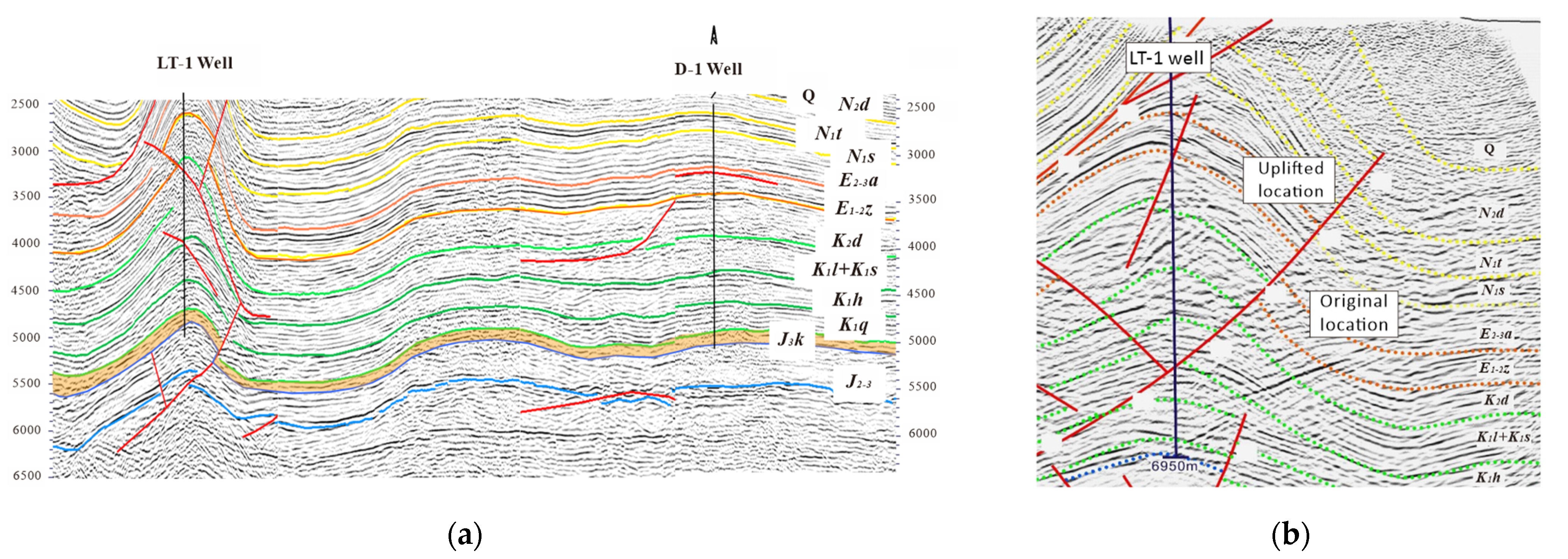
First, for a pilot well, such as the LT-1 well, in newly planned oil and gas blocks under investigation, there are no offset wells and no logging data available from the undrilled formations. The geomechanical analysis of the data and the further calculation of the mud window can only use the numerical results of the 3D geostress field for relevant analysis;

(2)

Second, when the ‘normal fault stress pattern’ appears within formations of the target block, the upper bound of the mud weight window is determined by the value of minimum horizontal stress. When a ‘reverse fault stress pattern’ appears, the upper bound of the mud weight window is determined by the value of overburden stress. In the oil and gas field at the southern edge of the Junggar Basin, due to the significant variation in elevation of the formation top, in different well sections of the same well, the ‘normal fault stress pattern’ and the ‘reverse fault stress pattern’ may exist at the same time: the upper part of the well section is in a normal fault stress pattern, the middle part is in a reverse fault stress pattern, and the lower part is again in a normal fault stress pattern. As a result, the analysis of the mud weight window obtained by the 1D analytical method is not accurate enough. So, it is necessary to use the numerical solution of the 3D geostress field to accurately calculate the mud weight window for a pilot well.

In the following sections, the geology of the target TS block, followed by the workflow for integrated analysis of 3D geostress and 1D geomechanical analysis of a well in a new gas field, is introduced. Then, the integrated analysis of the 3D geostress of the TS block and 1D geomechanical analysis of the LT-1 well are presented, which includes: (1) numerical analysis of the 3D geostress of the TS block; and (2) integrated 1D geomechanical analysis of target well LT-1. Pore pressure prediction and calculation of the mud weight window for safe drilling are then presented. Finally, a summary and conclusions are given along with discussions on further work for improvement of the results of this integrated method.

2. Materials and Methods

2.1. Overview of the Geology of the Target Block

The TS block includes the Tu-1 well and others that have been drilled with the shallower upper reservoir as the target layer. Figure 1 shows a plane view of the TS block in which the relative position of the target LT-1 well can be seen.

Table 1. Geological stratification and lithology description of well LT-1.

Formation	Symbol	Bottom Depth (m)	Lithology Description	Stratum Dip Angle
ShaWan	N1s	372	Mudstone with conglomerate, unequally grained sandstone.	55~65° southward tilt
AJHH	Breakpoint 1	542	The upper part is mainly mudstone; the lower part is interbedded with an unequal thickness of mudstone and argillaceous siltstone.	55~65° southward tilt
	E2-3a	1497
ZNQZ	E1-2z	2052	The upper part is dominated by siltstone, argillaceous sandstone; the lower part is composed of gravel-bearing unequal-grained sandstone and glutenite.	5~10° northward tilt
DG	Breakpoint 2	2162	Gravel-bearing unequal-grained sandstone, glutenite, fine sandstone, siltstone, and argillaceous sandstone.	5~15° northward tilt
	K2d	2947
LMQ + SJK	K1l + K1s	3847	The upper part is siltstone and sandy mudstone; the lower part is interbedded with argillaceous siltstone, gray mudstone and siltstone.	5~15° northward tilt
HTBH	K1h	4627	The upper part is dominated by argillaceous siltstone; the lower part is dominated by brown mudstone and silty mudstone.	5~15° northward tilt
QSH	K1q Breakpoint	5327	Mudstone and argillaceous siltstone interbedded. Light gray powder-fine sandstone and fine sandstone developed at the bottom.	5~15° northward tilt
HTBH2	K1h	5922	The upper part is mainly grayish brown argillaceous siltstone; the lower part is composed of brown mudstone and silty mudstone.	5~15° northward tilt
QSH2	K1q	6660	Mudstone and argillaceous siltstone interbedded. Light gray siltstone fine sandstone and fine sandstone are developed.	5~20° northward tilt
KaRaZha	J3k	6920	Dominated by thick-layered light gray sandy conglomerate.	5~20° northward tilt
QiGu	J3q	6950	Dominated by layers of brown mudstone and sandstone with medium-thick layers of gray–green siltstone and fine sandstone.	5~20° northward tilt

shows the distribution of formations from the ground to the J₁q formation. The length and width of the block model are 20.5 km and 15.5 km, and the maximum depth is 12 km. The plane grid size is 500 × 500 m². The LT-1 pilot well’s target formations are mainly the lower oil and gas formations including the formation of a reservoir, formations of source rock, and formation of the caprock below 6000 m. At this depth of formations, those included are the Karaza formation, the SGH formation, and the lower Jurassic BDW formation at a depth of 8000 m. The target formations of well Tu-1 and other wells that have been drilled in the upper part are the KaRaZha formation and the ZNQZ formation. The vertical depths of drilled upper shallow wells in the area are between 3000 m and 4000 m.

Figure 2a shows the seismic profile of well LT-1 and the distribution of the main faults. The vertical axis shows the data in the time domain. It can be seen from Figure 2a that the faults in the TS block are mainly reverse faults and thrust faults. This means that the horizontal geostress component in the block will have a higher value. Among the strata traversed by the LT-1 well, the upper strata have undergone substantial uplift. This part of the strata has undergone the movement of compaction first, and then uplift. Red curves represent locations of faults. The calculation of the normal compaction curve of the strata needs special attention. It has the same slope with a noncompacted strata but a different depth.

Figure 2b shows the view of a section of a survey line across the LT-1 well. It can be seen in Figure 2b that the E_1-2z and K₂d are two sets formations that were uplifted the most among all the formations around the LT-1 well. The compaction trend line will be discussed in later sections.

Table 1 shows the description of the geological stratification and lithology of well LT-1 obtained from the analysis of seismic information. According to the results of the seismic interpretation, there are three sets of reservoir formations. It is indicated that the upper reservoir is in the Paleogene formation, the middle reservoir is in the Cretaceous formation, and the lower reservoir is in the Jurassic formation. It has been predicted that the gas reservoir section of the ZNQZ formation is 1497~2052 m, the gas reservoir section of the QSH formation is 6500~6660 m, and the gas reservoir section of the Jurassic KaRaZha formation is 6660~6920 m.

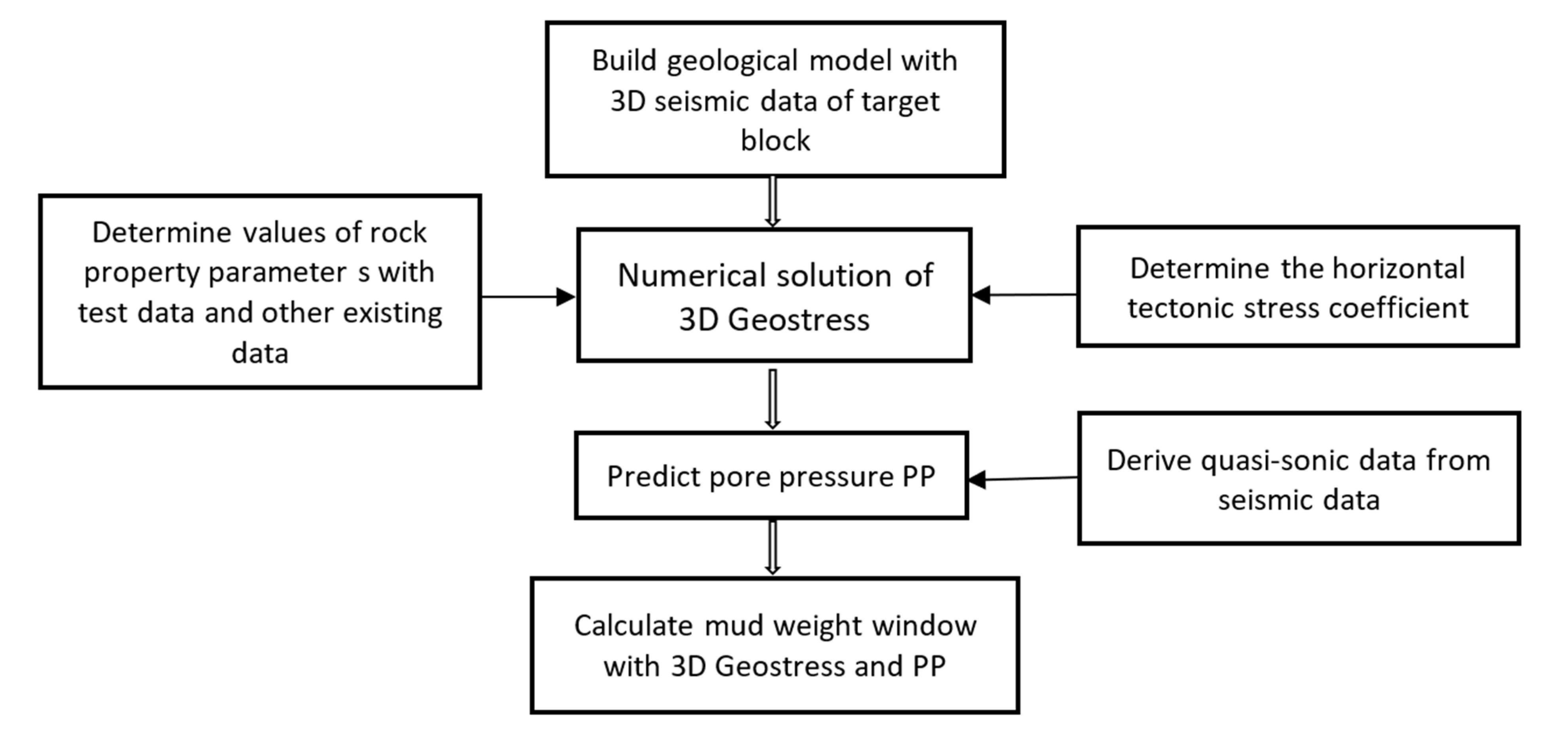
2.2. Workflow of the Integrated 1D Geomechanical Analysis of the Pilot Well and the 3D Geostress Analysis

The overall computational flow chart for pore pressure and mud window prediction with 3D geostress and formations’ interval velocity is shown in Figure 3.

This integrated analysis of the 3D geostress and 1D geomechanical analysis of the target well included a total of 4 main steps:

(1)

To build a geological model with input from the seismic data of the target block;

(2)

To perform a finite element analysis to obtain the numerical solution of the 3D geostress field;

(3)

The third step was the prediction of pore pressure. Tasks to be performed in this step included: (1) Extracting the formations’ interval velocity from the seismic data of the block and transferring it to sonic data; (2) Extracting the overburden pressure from the 3D geostress field and combining it with the sonic data to calculate the pore pressure curve. The Eaton’s method equation for the calculation of pore pressure is shown in Equation (1).

$$PP=OBG-ES;ES=\left(OBG-PP{G}_N\right){\left(\frac{d_{cO}}{d_{cN}}\right)}^E$$

(1)

where PP is pore pressure; OBG is the overburden gradient; ES is effective stress; PPGN is the hydrostatic pressure gradient, PPGN = 1.03 g/cm³; $d_{cO}$ is the sonic data; $d_{cN}$ is the sonic data of the normal compaction trend line; and E is the exponential index. The default value is 2.7. In the calculation presented here, the OBG is the vertical component ${\sigma }_v$ of the 3D geostress of the target block;

(4)

The fourth step was to synthetically use the solution of the 3D geostress of the target block and the 1D solution of the pore pressure of the pilot well to calculate the mud weight window of the target well.

Figure 4 shows the workflow for the calculation of the 3D geostress of the target block.

For simplicity. the value of the minimum horizontal stress, Shmin, of this 3D geostress was be used as the upper bound of the mud weight window. The lower bound of the mud weight window, called the shear failure gradient (SFG), was calculated with the other two principal components of the 3D geostress solution along with the cohesive strength and frictional angle of the formations. This process of calculation for the mud weight window is the same as that for a conventional method and further details can be found in [10].

3. Results of 3D Geostress and 1D Geomechanical Analysis

This section provides the application of the above principles for calculation of the 3D geostress of the target TS block, and the analysis for safe drilling of the pilot LT-1 well in the TS block. The TS block is located at the southern edge of the Junggar Basin, Xinjiang China.

3.1. Numerical Solution of 3D Geostress Field in TS Block

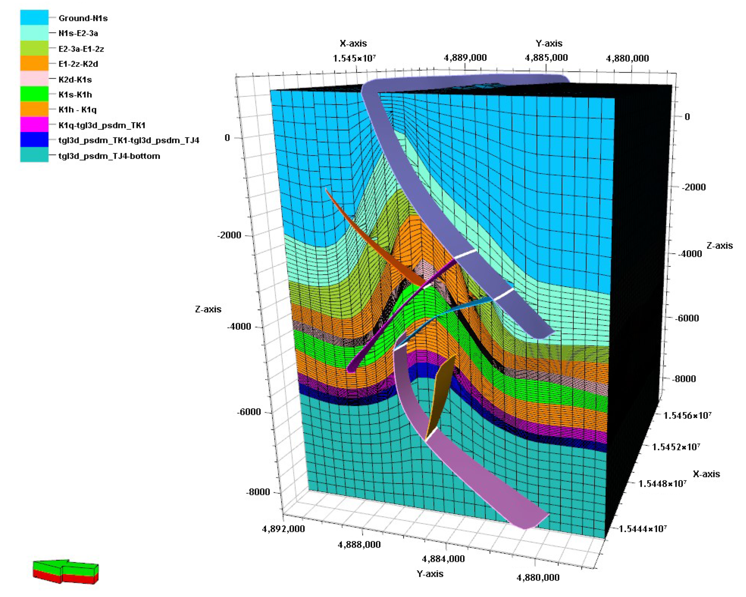
3.1.1. Finite Element (FE) Model

The geological properties of formations of the TS block and planar locations of existing wells in the block have been given in Figure 1 and Figure 2 and Table 1. Figure 5 below shows the 3D geological structure model of the TS block. It can be seen from Figure 5 that the block is cut by several thrust faults, and the anticline structure is obvious. Since there are many thrust faults in the block, the maximum horizontal geostress in the block is very high. In the process of orogeny, the fault is the location of displacement discontinuity. After hundreds of millions of years of geological periods, the current stress pattern is mainly determined by local structures such as anticline and gravity. The influence of tectonic movement is still there, but the magnitude of tectonic stress has obviously weakened with time.

When simulating the fault in the FE model, only the change in material properties is considered on both sides of the fault. The fault plane is not regarded as a fracture plane in a 3D space.

The finite element model given in Figure 6 completely inherits the stratigraphic structure given in Figure 5. Colors in Figure 6a indicate different formations of the model. The red shape in Figure 6b shows location of the LT-1 well. This finite element mesh includes 370,000 nodes and approximately 90,000 C3D20R-20-noded high-order elements. The boundary conditions of the Abaqus FE model are given as the following:

• The bottom surface and four side surfaces have normal zero displacement boundaries;
• The top surface is the ground and is a free surface.

The gravity is set as the initial load. The initial geostress field and gravity load form a balanced initial geostress field. Application of an initial stress field is realized by Abaqus software directly assigning values to the stress points of each element, and then performing elastic equilibrium iteration [14].

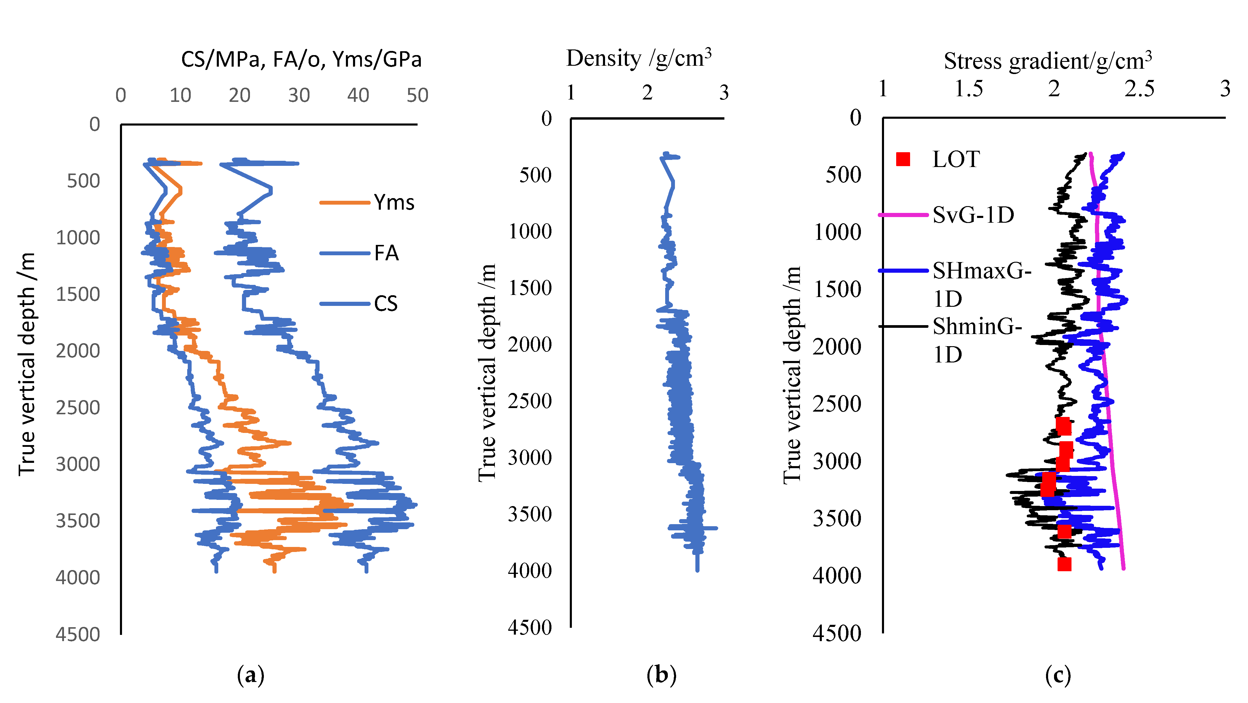
3.1.2. The 1D Geomechanical Analysis of the Tugu-1 Well and Initial Input Data for the 3D FE Model

The Tugu-1 well is an existing well at shallow formations of the TS block. In addition, it cannot provide data for the target formation of the pilot LT-1 well, which is below 5000 m; the 1D geomechanical solution of this Tugu-1 well provides data for formations in the upper part of the LT-1 well.

Solutions of the 1D geomechanical analysis of the Tugu-1 well are shown in Figure 7a–c. LOT (leak-off test) data indicate that the value of the minimum horizontal stress gradient ShminG is equal to the value of the fracture gradient. By definition, the fracture gradient is the value of the mud weight at which fractures within formations around the borehole start to open, and the fluid in the LOT starts to leak-off from the borehole into the formations. In theory, the fracture gradient is equal to the value of the minimum horizontal stress gradient. In this way, the curves of ShminG in Figure 7 are validated.

Based on the results of the 1D geomechanical analysis of the Tugu-1 well, the distribution of the lateral stress coefficients Lsr-1 and Lsr-2, which is the ratio of the 2 horizontal stress components to the vertical stress [14,15], along the vertical depth, is derived and is used as input data for the Abaqus FE model. At the formation K₁s-K₁q, which is at a depth interval from 2500 m and deeper, the value of the maximum horizontal stress SHmax is smaller than the value of the vertical stress Sv. Therefore, at this depth interval the stress pattern is a normal fault stress pattern.

At the location of target well LT-1, Figure 5 shows that location of the reverse fault structure is shallower than that at the Tugu-1 well. At the LT-1 well, the reverse fault stress pattern occurs within formation K1s-K1q, which is at a depth of 2700 m to 8000 m. This factor was considered in the input data for the TS block.

Based on the 1D geomechanics solution obtained with Tugu-1 and other existing wells, effective stress ratio k0 values were determined and they are listed in

Table 2. Values of k0 for the FEM model.

TVD/m	k0
197	0.8
2722	0.6
3000	2
3480	2
3551	2
4008	2
4309	2
4772	2
4808.37	3
5100	3.5
5135.39	3
5244	2
7105.57	1

. With Shmin as the minimum horizontal stress, Sv as the vertical stress, and pp as the pore pressure, the effective stress ratio k0 = (Shmin-pp)/(Sv-pp). It varies with the depth TVD, as shown in Table 2. The values listed here are approximately calculated by matching the reference drilling mud weight when calculating the collapse pressure of adjacent wells. At a depth of 3000~5200 m, the value of Shmin caused by tectonic stress is greater than the vertical stress. Due to the high pore pressure, the value of k0 is obviously greater than 1.

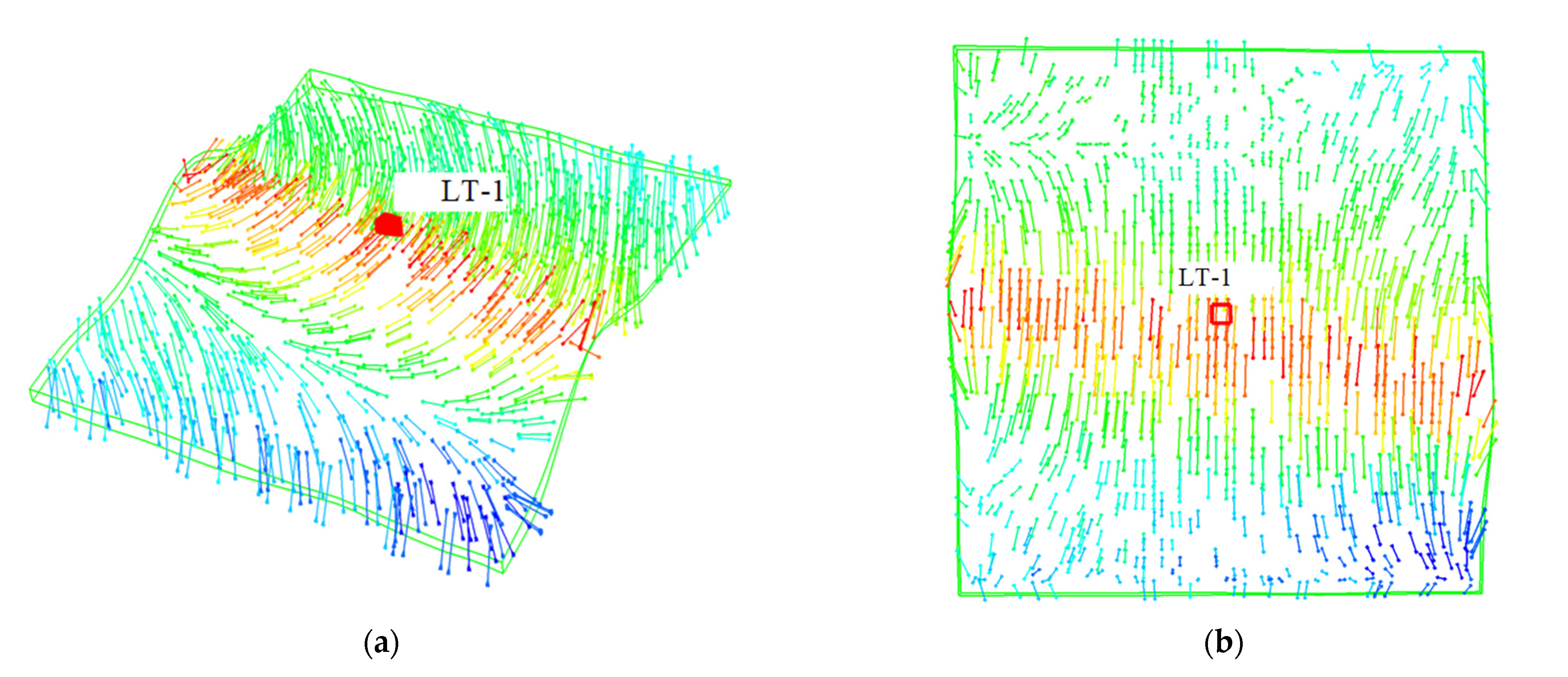
3.1.3. Numerical Solution of the 3D Geostress Field of the Target TS Block

Figure 8 shows the distribution of the orientation of the maximum principal stress Smax within the target formation J₃q. The red symbol indicates location of the LT-1 well. Figure 8a is a 3D distribution of Smax, and Figure 8b is a plane view of the distribution of Smax. The maximum horizontal principal stress SHmax is the maximum horizontal principal stress at the position of well LT-1, as shown in Figure 8b. At other locations, except at the top of the anticline, the orientation of SHmax is not horizontal.

Due to the variation in elevation of the formation top, the distribution of the maximum principal stress Smax in the target formation of well LT-1 varies with the horizontal position, as shown in Figure 8a. The direction of the SHmax at the position of LT-1 at the top of anticline is basically in a north–south direction. At this location, the vertical stress component is the minimum principal stress component, and the stress pattern is a reverse fault stress pattern.

The values stress components at the points of trajectory of the target LT-1 well can be extracted from the 3D geostress solution of the TS block. Figure 9 shows the values of the three principal stress components of the geostress field in the form of the stress gradient at LT-1. The curve of Sv-1D is the value obtained from the density integral over the entire well length. The other three curves are plotted from the numerical results of 3D numerical calculations. It can be seen in Figure 9 that the values of Sv-1D ad Sv-3D have a discrepancy. This discrepancy is caused by tectonic movement as well as factors of anticline structures of the formation.

3.2. Pore Pressure and Mud Weight Window Prediction of the LT-1 Well Based on 3D Geostress and Layer Velocity

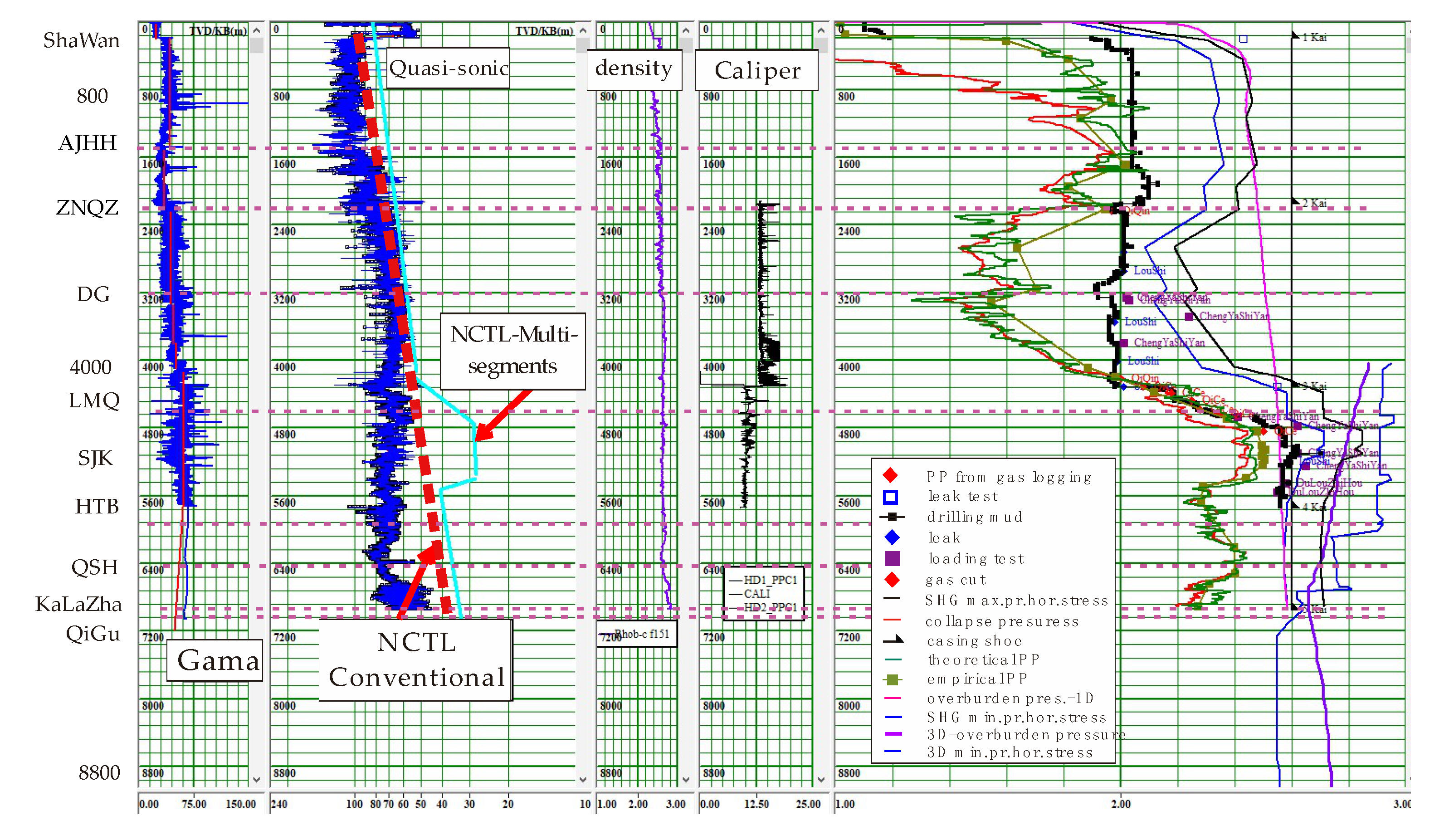
3.2.1. Pore Pressure Prediction

As the third step of the integrated analysis of 3D geostress and 1D geomechanical analysis, pore pressure prediction of the target LT-1 well was performed on the basis of numerical solution of the 3D geostress. The solution of the vertical stress gradient SvG-3D shown in Figure 9 was used. As there is no offset well in this TS block, the quasi-sonic data derived from the interval velocity of the target block was used as the sonic data for the LT-1 target well, as is shown in track 2 from the left in Figure 10. The software Drillworks v2020 was used for this 1D geomechanics calculation.

The data from the formation bearing test (FBT) are shown in Figure 9. The purpose of this test is to confirm that the value of a given mud weight density is safe for further drilling. This test is similar to the popular formation integrity test, but not exactly the same. The maximum value of this FBT was 2.65 g/cm³, which is obviously higher than the Sv-1D: the vertical stress obtained by density integration over depth. This indicates that the 1D solution of vertical stress was smaller than the real value of vertical stress, which was larger than the value of 2.65 g/cm³ at this depth section. Furthermore, this indicates than the 3D numerical solution of the vertical stress SvG-3D was accurate.

Discrepancy between the values of vertical stress obtained by the 1D method, Sv-1D and SvD-3D, and those obtained by the 3D numerical method was mainly due to the impact introduced by tectonic stress, and there was little impact from the local anticline structure. Sv-1D is calculated by the density integral over depth, and it does not account for tectonic stress. However, SvG-3D is obtained with magnitude of tectonic factor tf = (SHmax − Shmin)/(Sv − Shmin) = 1.3 to 1.5. Primary numerical results indicated that: if the magnitude of tf increases, the values of all three principal stress components will increase due to the existence of an anticline structure.

In Figure 10, the purple line indicates the depth of the bottom of each formation.

The normal compaction trend line (NCTL) is an important factor in the prediction of pore pressure [10]. The NCTL is a set of empirical lines in the space of the logarithm of the sonic data vs. depth, and it represents the value of sonic data at points of rock formation along the well trajectory after millions of years of sedimentation and compaction due to the gravity of overburdened formations. Usually, in Eaton’s method [10], this NCTL is empirically presented as a straight line.

In the case of the TS block and LT-1 well, formations were compacted first and then were lifted to a higher elevation by tectonic movement, as can be seen from Figure 2a,b. Consequently, the NCTL formations at the depth interval from 4500 m to 5500 m cannot be a straight line. Several line segments must be used to form a set of the NCTL that can properly reflect the compaction trend in formations at this specific depth interval. This set of multi-segmented NCTL is shown in track 2 from the left in Figure 10.

Caliper logging data, shown in track 2 from the right, illustrates that an obvious borehole enlargement occurred at sections around the depth of 4000 m. The data point leak at 4000 m, in track 1 from the right, indicates that there was mud loss during drilling, and there are plenty of high conductive natural fractures at this depth location. According to the record of drilling issues, hydraulic plugging was used in order to achieve an enhanced mud weight window for this section.

The rock density values of formations are shown in track 3 from the left, and they were calculated from the quasi-sonic data. This set of density data was validated by the rock density parameters obtained from the logging density data for the same type of formations in a neighboring block. Currently, the actual mud drilling has reached a depth close to 5800 m. Near the vertical depth of 4000 m, the borehole wall is seriously enlarged, which leads to poor logging data quality. Near 2300 m, there was a gas invasion event.

With the input data prepared as described above, the pore pressure prediction was performed. The results of the predicted pore pressure for this pilot LT-1 well are shown in track 1 from the right in Figure 10. The pore pressure coefficient values of the formations along the trajectory of the LT-1 well are listed in

Table 3. Mud weight window prediction for each formation in well LT-1.

Formation	Formation Bottom Depth/m	Pore Pressure Gradient g/cm3	Shear Failure Gradient g/cm3	Fracture Gradient g/cm3	Mud Weight Window g/cm3
Shawan N1s	172	1.0–1.1	1.0	1.85–2.0	1.1–1.85
AJHH E2-3a	188	1.0–1.1	1.0	2.0–2.1	1.1–2.0
AJHH2 E2-3a	1474	1.7–1.9	1.0–1.9	2.2–2.3	1.9–2.2
ZNQZ E1-2z	2100	1.8–1.98	1.75–1.98	2.3–2.35	1.98–2.3
DG K2d	2147	1.98	1.8	2.13	1.98–2.13
DG2 K2d	3250	1.6–1.97	1.45–1.9	2.05–2.23	1.97–2.05
LMQ K1l	4309	1.5–1.99	1.4–1.99	2.1–2.58	1.99–2.1
LMQ2 K1l	4578	1.99–2.3	1.99–2.25	2.68–2.81	2.25–2.68
SJK K1s	5240	2.3–2.55	2.3–2.45	2.74–2.79	2.55–2.74
HTBH K1h	5746	2.25–2.5	2.3–2.45	2.65–2.77	2.5–2.65
HTBH2 K1h	5922	2.25–2.35	2.25–2.35	2.63	2.35–2.63
QSH K1q	6660	2.3–2.4	2.3–2.4	2.61	2.4–2.61
KaLaZha J3k	6920	2.2–2.35	2.2–2.35	2.55	2.35–2.55
QiGu J3q	6950	2.2–2.35	2.2–2.35	2.5	2.35–2.5

.

The pore pressure curve in the rightmost column of Figure 10 shows the following trend at the target LT-1 well: (1) The uppermost ShaWan formation is at normal pressure. The pore pressure gradient rapidly increased to over 1.8 g/cm³ after entering the AJHH formation, then gradually decreased to approximately 1.5 g/cm³ in the ZNQZ formation and the DG formation, and then gradually increased to approximately 2.5 g/cm³ in the LMQ and SJK formations. The pore pressure gradient decreased in the HTBH formation, and increased in the QSH formation, and decreased again in the KaLaZha formation. However, its value remained between 2.2 and 2.4 g/cm³.

The current drilling issue information has proven that the predicted pore pressure values are in good accordance with the phenomena observed during drilling practices; the gas invasion event indicates that the pore pressure value equaled the mud weight gradient actually used during the drilling operation, which is shown as a black symbol in Figure 10.

3.2.2. Calculation of the Mud Weight Window for Safe Drilling

As the fourth step of the integrated analysis, the calculation of the mud weight window for safe drilling was performed for the target LT-1 well. The equations and theory for conventional calculation have been described by the authors [10,11]. The solution of 3D geostress was used here to calculate the lower and upper bound of the safe mud weight window instead of the solution of the conventional 1D geomechanical analysis.

The upper bound of the safe mud weight window took the value of the minimum horizontal stress ShminG-3D as an approximation, as shown in Figure 10 and Table 2. The lower bound is regarded as the shear failure gradient. Its input data include three principal stress components and rock strength parameters, including the cohesive strength and internal frictional angle of the points along the trajectory of the LT-1 well.

The resultant solution of the upper and lower bounds of the mud weight window for the LT-1 well is shown in track 1 from the right in Figure 10, and its values are listed in Table 3.

At the time of undertaking this study, the actual drilling operation had reached a depth close to 5800 m. The information regarding drilling issues proved that the predicted mud weight window values were in good accordance with the phenomena observed during drilling practices: (1) No borehole collapse occurred when the actual value of mud weight used in the drilling operation was larger than the value of the lower bound of the mud weight window; and (2) Mud leak-off occurred when the actual value of the mud weight used in the drilling operation approached the value of the upper bound of the mud weight window.

However, in track 1 from the right in Figure 10, it can be seen that, at a depth 4400 m, the pore pressure value obtained by gas logging was obviously higher than the value of the 1D overburden pressure, which was calculated by the integral of gravity over the depth. This indicates that the value of local stress components is seriously impacted by the anticline structure. Moreover, it indicates that the tectonic stress is high. These phenomena show that the 3D numerical solution of geostress is able to select the minimum principal stress component as the upper bound of the mud weight window under all kinds of stress pattern. This is one of the advantages of using the numerical solution of the 3D geostress field to predict pore pressure and to calculate the mud weight window.

4. Discussion

Aiming for a geomechanical solution for the safe drilling of a well in the exploration of a new oil and gas block with no logging data from existing wells, an integrated workflow for 1D geomechanical and 3D geostress analysis was proposed. The major steps of this workflow included numerical calculation of the 3D geostress of the target block and 1D geomechanical analysis of the pilot well, which applied the numerical solution of 3D geostress as an input to the 1D geomechanical analysis. In this way, the impact of high tectonic stress as well as the influence of local geostructures such as anticline and synclines were considered in the prediction of pore pressure, as well as in the calculation of the mud weight window for safe drilling.

With this proposed workflow, integrated 1D geomechanical analysis was performed for the pilot LT-1 well within the target TS block at the southern edge of the Junggar Basin, Xinjiang, China. The predicted results of pore pressure and the mud weight window were in good accordance with data obtained from the drilling operation through drilled well sections. This shows that this proposed method is accurate and feasible for the safe drilling of a pilot well at the southern edge of the Junggar Basin.

It should be noted that due to the existence of natural fractures, especially the existence of high conductivity fractures of this field under exploration, mud leakage may still occur despite that the value of the mud weight being within the calculated safe mud weight window, i.e., mud loss during drilling may occur with a mud density obviously smaller than that of the minimum horizontal stress Shmin. In this case, hydraulic plugging is the solution to stop mud loss during drilling, and it is necessary to perform analysis of the extended mud weight window. This will be a topic for further investigation in this area.

5. Conclusions

Due to the technical limits of 1D geomechanics analysis and that of 3D geostress calculation, it is not possible to use only one of them to obtained accurate solutions of pore pressure prediction as well as geostress: vertical stress calculated by 1D density integral over depth is not accurate for regions with high tectonic stress, and further results in inaccuracy of predicted pore pressure. Multi-segments of compaction trend line for regions with complicated fault and formation uplift is must to be used in the Eaton method for pore pressure prediction. Integrated workflow, which integrates merits of both 1D and 3D geomechanics method, is a powerful tool for pore pressure prediction and mud weight window’s calculation of an exploration well.

The target well LT-1 has been successfully drilled. This indicates the solution of pre pressure and mud weight window presented here are practical, and the model and workflow of this work are proper.

References

1. Gao, Z.Y.; Shi, Y.X.; Feng, J.R.; Zhou, C.M.; Luo, Z. Lithofacies paleogeography restoration of Jurassic to lower Cretaceous in southern margin of Junggar Basin, NW China. Pet. Explor. Dev. 2022, 49, 20220204. [Google Scholar] [CrossRef]
2. Lin, Z.; Sun, Z.; Hu, H.; Xu, K.; Lei, C. Pore pressure distributional characterization of shale gas reservoir in WR block of Sichuan basin. Prog. Geophys. 2021, 36, 2045–2052. [Google Scholar]
3. Chilingar, G.V.; Serebryakov, V.A.; Robertson, J.O., Jr. Origin and Prediction of Abnormal Formation Pressures, Development in Petroleum; Science Book Series; Elsevier: Berkeley, CA, USA, 2002; Volume 50. [Google Scholar]
4. Shen, G.Y.; Clemmons, C.; Shen, X.P. Integrated 1-D workflow for pore-pressure prediction and mud weight window calculation for subsalt well sections. In Proceedings of the 49th US Rock Mechanics/Geomechanics Symposium, San Francisco, CA, USA, 28 June–1 July 2015. Paper NoARMA 15-097. [Google Scholar]
5. Xu, J.L.; Wang, J.; He, D.B. A method for calculating pore pressure coefficient directly using ADCIGS. In Proceedings of the CPS/SEG International Geophysical Conference & Exposition, Beijing, China, 24 April 2018. Electronic Papers. [Google Scholar]
6. Uhunoma, O.A.; Olalere, O. Combining porosity and resistivity logs for pore pressure prediction. J. Pet. Sci. Eng. 2021, 205, 108819. [Google Scholar]
7. Wang, Z.C.; Wang, R.H. Pore pressure prediction using geophysical methods in carbonate reservoirs: Current status, challenges and way ahead. J. Nat. Gas Sci. Eng. 2015, 27, 986–993. [Google Scholar] [CrossRef]
8. Mannon, T.; Salehi, S.; Young, R. Seismic frequency versus seismic interval velocity based pore pressure prediction methodologies for a near salt field in Mississippi Canyon, Gulf of Mexico: Accuracy analysis and implications. In Proceedings of the IADC/SPE Drilling Conference and Exhibition, Fort Worth, TX, USA, 4–6 March 2014. Paper No SPE 167915-MS. [Google Scholar]
9. Cai, W.J.; Deng, J.D.; Zhang, J.F. Three-dimensional pore pressure prediction and visualization of reef limestone reservoirs in Indonesia A oilfield. Sci. Tech. Eng. 2021, 21, 8863–8869. (In Chinese) [Google Scholar]
10. Mouchet, J.P.; Mitchell, A. Abnormal Pressure while Drilling; Editions Technip.: Paris, France, 1989. [Google Scholar]
11. Wang, H.T.; Kou, Z.H.; Guo, L.L.; Chen, Z.T. A semi-analytical model for the transient pressure behaviors of a multiple fractured well in a coal seam gas reservoir. J. Pet. Sci. Eng. 2021, 198, 108159. [Google Scholar] [CrossRef]
12. Kou, Z.H.; Zhang, D.X.; Chen, Z.T.; Xie, Y.X. Quantitatively determine CO2 geosequestration capacity in depleted shale reservoir: A model considering viscous flow, diffusion, and adsorption. Fuel 2022, 309, 122191. [Google Scholar] [CrossRef]
13. Kou, Z.H.; Wang, H.; Alvarado, V.J.; McLaughlin, F.; Quillinan, S.A. Method for upscaling of CO2 migration in 3D heterogeneous geological models. J. Hydrol. 2022, 613, 128361. [Google Scholar] [CrossRef]
14. Dassault Systemes. Abaqus Analysis User’s Manual, 14th ed.; Dassault Systemes Simulia Corp.: Providence, RI, USA, 2011; Volume IV. [Google Scholar]
15. Shen, X.P.; Williams, K.; Standifird, W.B. Enhanced 1D prediction of the mud weight window for a subsalt well, deepwater GOM. Soc. Pet. Eng. J. 2014, 9. [Google Scholar] [CrossRef]
Figure 1. Planform of the TS block: target well and the relative position of existing wells.
Energies 16 00806 g001
Figure 2. (a) Profile and structure of a main survey line of Tugulu anticline of TS Block. (b) A sectional view of a survey line across well LT-1.
Energies 16 00806 g002
Figure 3. Illustration of workflow of integrated 1D geomechanical analysis of pilot well and 3D geostress analysis.
Energies 16 00806 g003
Figure 4. Workflow for calculation of 3D geostress.
Energies 16 00806 g004
Figure 5. Geological structure model of the TS block.
Energies 16 00806 g005
Figure 6. ABAQUS finite element model of TS block: (a) Model grid. (b) Grid of reservoir formation J3q.
Energies 16 00806 g006
Figure 7. Results of 1D geomechanical analysis of Tugu-1 well in TS block: (a) Distribution of CS, FA, and E along well depth; (b) density of rock; (c) SHmin, SHmax, and Sv.
Energies 16 00806 g007
Figure 8. Distribution of the Smax and SHmax of target formation J3q in block LS-1. (a) 3D view of the stress Smax distribution. (b) plane view of the stress SHmax distribution.
Energies 16 00806 g008
Figure 9. Stress gradient as a function of vertical depth at well LT-1.
Energies 16 00806 g009
Figure 10. Pore pressure prediction and mud weight window results based on 3D geostress and velocity analysis.
Energies 16 00806 g010