Abstract
Mixed and multi-model assembly line sequencing problems are more practical than single-product models. The methods and selection criteria used must keep up with the constantly increasing level of variability, synchronize flows between various—often very energy-intensive production departments—and cope with high dynamics resulting from interrupted supply chains. The requirements for conscious use of Earth’s limited natural resources and the need to limit energy consumption and interference in the environment force the inclusion of additional evaluation criteria focusing on the environmental aspect in optimization models. Effective sustainable solutions take into account productivity, timeliness, flow synchronization, and the reduction of energy consumption. In the paper, the problem of determining the sequence of vehicles for a selected class of multi-version assembly lines, in which the order restrictions were determined taking into account the above criteria, is presented. Original value of the paper is the development of the Grey Wolf Optimizer (GWO) for the mixed-model assembly lines sequencing problem. In the paper, a comparative analysis of the greedy heuristics, Simulated Annealing and GWO for a real case study of a mixed vehicle assembly line is presented. The GWO outperforms other algorithms. Overall research performance of the GWO on the sequencing problem is effective.
1. Introduction
Industry uses huge amounts of energy to transform resources into products or services, which increases competition for energy resources and has a huge impact on the environment [1,2]. The industrial sector, after transport and households, is one of the largest energy consumers in the EU, accounting for 25.6% of final energy consumption in 2021 [3]. By comparison, in the United States, one of the most industrialized countries, the industrial sector accounted for 33% of total U.S. energy consumption in the same year. Moreover, energy consumption forecasts until 2050 for the USA indicate that the largest percentage increases should occur in the industrial sector, where energy consumption is projected to increase by as much as 32% [4,5]. At the same time, the observed increase in energy prices is becoming a growing problem. This is becoming a challenge for manufacturers, especially in the automotive industry, which in recent years has also had to deal with global supply chain problems, such as global shortages of semiconductors. In this context, car manufacturers focus on developing long-term development strategies aimed at significantly improving the energy efficiency of production, further driven by global trends towards minimizing negative impact on the environment and so-called green and sustainable production. This is a particular challenge considering that modern cars are equipped with increasingly complex systems, making them greener, safer, and smarter, but it also contributes to a significant increase in the complexity of the vehicle itself and its production process. Of course, this increase in complexity directly affects the energy needs of production processes. Depending on the research, it is estimated that the production of today’s vehicle requires an estimated energy input of 62 GJ, of which approximately 42 GJ is energy consumed during extraction and material production, while the processes of producing parts and assembling the vehicle consume 12 and 8 GJ, respectively [6]. However, data presented by the European Automobile Manufacturers’ Association (ACEA) show that the specific energy consumption during car production is approximately 10 GJ [7].
The above-mentioned increase in the complexity of vehicles and the resulting increase in energy demand in production processes also increase the variability of the range and diversity of manufactured products. In the case of the automotive sector, this diversity is becoming an immanent feature not so much in relation to unit and small-series production but also increasingly to large-scale and mass production (mass customization). With regard to assembly lines, this variability and the associated level of flexibility are classified in the literature according to the number of models and versions, as single-model, multi-model, and mixed [8,9]. The production of different models on the same assembly line allows for significant energy and cost savings also thanks to the arbitrary combination of series, batches, and different volumes of individual models. Of course, the greatest flexibility is provided by solutions based on the mixed-model concept, but their wide application requires the simultaneous development of methods and techniques in the area of flow management and organization. The required increase in productivity and flexibility while maintaining or even reducing energy consumption can also be achieved by using the numerous opportunities offered by the fourth industrial revolution (Industry 4.0). They affect the so-called agility of the system, and thanks to ongoing production tracking and ensuring traceability and comprehensive information flow, they allow for dynamic sequencing of vehicles on the assembly line in response to current conditions [10,11].
Sequencing allows manufacturers to determine the order in which they deploy product variants or models depending on current requirements and the state of subsystems associated with the main product flow. In practice, this makes it possible to shorten the so-called planning time horizon, i.e., the period during which the established sequence can no longer be changed, which in turn reduces the number of costly and energy-intensive product withdrawals during the implemented sequence (e.g., due to the lack of required components or production capacity). Changes and imbalances in the sequence often lead to exceeding the availability of time at a given assembly station, which in turn results in frequent line downtime and ultimately non-compliance with production standards. This, in turn, forces overtime to make up for lost time and thus reduces energy efficiency per vehicle unit. In a multi-model assembly line, different models are assembled, and each model may require different assembly operation times.
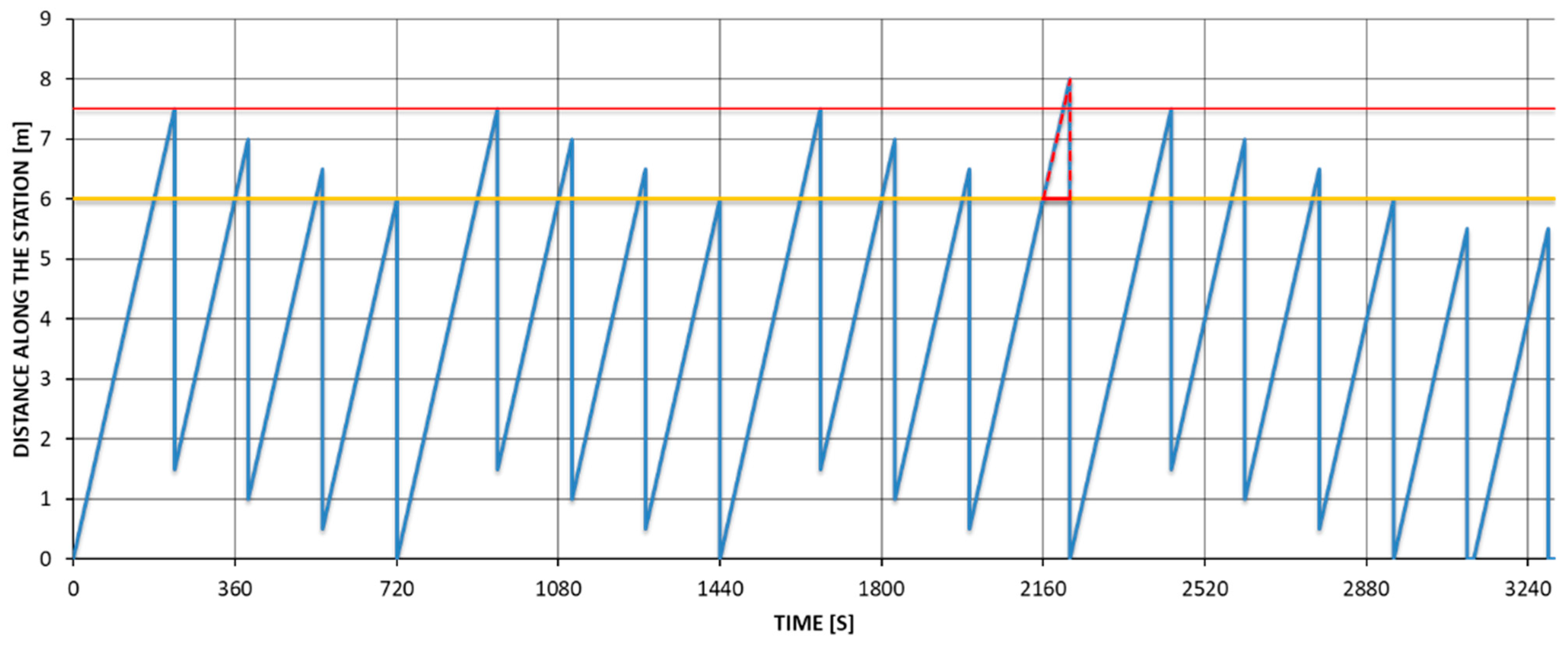
Depending on the model option, the vehicle may require additional time for individual assembly stations on the assembly line. Therefore, the vehicle is assumed to exceed the average time of assembly operations at the stations and is called a work-intensive model or version. In the case of successive operation of models with a longer operation time, the model completion time is moved to downstream of the station (the area between the yellow and red lines in Figure 1). This is especially important when an assembly line consists of a number of stations linked by a conveyor or an AGV moving at a constant rate. In cases of several work-intensive models being assembled consecutively at the same workstation, work overload may occur and should be compensated for (Figure 1). If the allowed area is exceeded, operators must stop the conveyor or AGV to complete the unfinished operation (beyond the red line in Figure 1) [12,13]. This situation (overrun and waste of time and energy) is often associated with exceeding the sequencing rule regarding the maximum number of vehicle occurrences with a specific option among a specified number of consecutive sequence positions [8,12].

Figure 1.
Operator movement at a workstation in the mixed-model line.
Therefore, manufacturers are looking for new, effective, and easy-to-implement (and later adopt to new requirements) computer-aided sequencing methods and tools for multi-model assembly lines in conditions of high variability and time pressure. In the literature, the sequencing problem considered in this paper is traditionally referred to as the car sequencing problem (CSP) [14,15]. However, this nomenclature (resulting from the origins of this class of problems) does not, of course, limit the scope of applicability of the group of methods solving this problem to assembly systems in the automotive industry—they can be (and are) also used in other industries. In recent years, for the above-mentioned reasons, the problem of sequencing assembly lines, also in the context of improving the energy efficiency of existing production systems, has become the subject of an increasing number of scientific publications [16,17,18].
The objective of this paper is to develop a sequencing method—in order to reduce overruns and waste of time and thus save energy—in which the traditional approach of specifying a representation of the problem proportion constraint (in terms of the number of vehicles that may contain an option in a sequence of a given length) is tightened to one vehicle in each subsequence. Moreover, for operational reasons, we move away from the traditional objective function based on minimizing the number of constraint violations within a sequence in favor of minimizing the sum of the degree of constraint violations. The motivation for this approach is presented in the next section. We propose the use of previously successfully applied algorithms in solving the traditional problem and a new, previously unused algorithm. For this reason, three approaches are examined to solve the analyzed problem: a method based on a dedicated greedy algorithm, a simulated annealing algorithm with various parameters, and a grey wolf optimizer.
Exact methods are effective in finding optimal solutions to small and medium-sized problems [19]. When it comes to solutions for large CSPs, metaheuristic algorithms play a leading role. Among metaheuristic algorithms, tabu search [19] and simulated annealing [20,21] methods are popular. Ant colony optimization [22] and genetic algorithms [23,24] are also known from the literature. In recent years, new metaheuristics have been proposed for solving scheduling problems: smart swarm optimization [25], flame moth optimization algorithm [26], salp swarm algorithm [27], and grey wolf optimizer [28]. In scheduling problems, GWO can obtain the most well-known solutions in most scheduling problems [28]. The algorithm based on GWO proposed in [28] outperformed the above-mentioned new metaheuristics and self-learning genetic algorithm [29], and it was proven that each grey wolf individual of GWO has simple intelligence. In many cases, scheduling problems are based on the permutation of production tasks just as CSP is based on the permutation of car versions, so the authors of the paper need to investigate the applicability of GWA for CSP. To the authors’ knowledge, the GWO has not been applied in CSP so far.
The original contributions of the paper are the proposed evaluation function for the tightened car sequencing problem, minimizing the degree of constraint violations and the developed grey wolf optimizer (GWO) with encoding, decoding, differentiating, and selection methods for solving the car sequencing problem with constraints in generating vehicle versions.
2. Problem Definition and Solution Methods
The problem of vehicle sequencing on the final assembly line, referred to in the literature as the car sequencing problem (CSP), is considered [14,15,22,30]. The proposed formal mathematical models of CSP have evolved since the 1980s along with the evolution of assembly line organization related to the need to produce many models and their variations (versions) in different volumes on the same line (mixed-model and multi-model). The CSP problem was first described in [31]. In the traditional approach, the set of considered constraints concerns the possible options for a given product version, and the definition of the so-called p/q ratio. In the ratio, in any subsequence of q vehicles sequentially planned for assembly on the line there may be at most p versions of vehicles in which a given option is present. CSP is defined as a tuple [15]:
where:
(V,O,p,q,r)
- V = {v1,…,vn}—set of vehicles to be made,
- O = {o1,…,om}—a set of different options that may be available in a given version of the product,
- p:O ⇒ ℕ and q:O ⇒ ℕ—capacity constraint associated with each option oi ∈ O—for any sub-sequence of products qi, there can be at most pi vehicles requiring option oi,
- r:V × O ⇒ {0,1}—option requirements,—for each vehicle vj ∈ V and for each option oi ∈ O, rij = 1 if oi is required for vehicle vj and rij = 0 if oi is not present.
Solving the CSP problem comes down to finding the order of the elements of the set V that meets the given constraints, thus determining the order in which the vehicles (or more precisely, their versions associated with the option set) are assembled on a given line. In particular, the question of whether it is possible to find a sequence that satisfies all the p/q constraints must be answered. The p/q constraints were originally related to the adopted assembly method, in which stations dedicated to the assembly of a given option were designed for a specific maximum percentage of vehicles moving along the line [15,31]. In such a case, in order to be able to install a specific percentage of vehicles (with an even workload of employees) at selected assembly stations, it is necessary to plan a multi-person team of operators and design the length of the stations as a multiple of the distance travelled by the vehicle during the line takt time [31].
In currently designed assembly lines, especially in the automotive industry, the described mode of operation is very rare. There is practically no movement of operators to subsequent assembly stations during work. Requirements related to additional labour consumption of the vehicle in which a given option is to be installed are taken into account in the determined average length of stations for the lines on which the vehicle moves at a constant speed (and thus in the average line cycle). This approach assumes the possibility of crossing the station zone for the so-called heavy versions (versions with an option required during assembly, causing an increase in labour consumption above the average for a given station), which is levelled during assembly operations for (usually several) consecutive so-called light vehicles (see Figure 1). Therefore, an extremely undesirable situation is two consecutive heavy versions for a given station in a row of vehicles. The authors observed this approach to the design and organization of flow on assembly lines, especially in heavy vehicle assembly plants.
In practice, for a given set of options (and the corresponding vehicle versions, already at the line design stage), manufacturers determine the minimum number of versions not containing a given option, which should follow the version containing it. This guarantees that the planned line capacity will be achieved. Therefore, in order to meet the requirements of today’s manufacturers, we propose modification of the constraints in the traditional model (1) in such a way that the p constraint always takes the value 1. This corresponds to a tightening of the pi/qi constraint set to 1/qi and describes the above situation, in which the planner defines the number of vehicles without options in the sequence (q − 1) that should occur between every two vehicles having a given option. Thus, the modified SCP problem is a tuple:
(V,O,1,q,r)
The sequence of product versions is defined as an ordered m × n matrix S, whose columns correspond to the vectors of individual product versions r:
where i—option number that may appear in a given vehicle version, i = 1…m, m—number of options, j—jth position in the version implementation sequence in the production cycle, j = 1…n, n—number of vehicles to be completed.
S = [sij], sj ∈ rj
Thus, the restriction shown in Constraint (4) imposes that only one vehicle may contain the option i in a sequence of qi length:
where gap(ij)—a gap in the sequence S between product vj and the next product with option oi.
We also propose another modification with respect to the traditional approach to the definition of CSP problem. It is assumed there [15,22,30] that different cars of V may require the same option configuration, and all cars requiring the same option configuration are clustered in the same car class. More precisely, there are k different classes of cars, so V is divided into k subsets such that all vehicles in the same subset Vi require the same option configuration [15]. In our model, we do not define the division of the set of vehicles into classes. This is motivated by today’s industrial practice, in which not only different versions of the same model are assembled on the same line but also different models with corresponding options. This causes much greater variability and freedom in formulating sets of input vehicles for the sequencing process, in which for a single work shift there may practically be no two identical sets of options in different vehicles.
The evaluation of the established sequence must reflect the degree to which the specified performance constraints are met (4). In industrial practice, they are the result of the assumptions made when designing the line as well as the current parameters (and disturbances) of the line operation, including production volume, component availability, staff, etc. The approaches proposed for solving the traditional CSP can be mainly split between treating it as a feasibility problem and treating it as an optimization one [8,22]. The first group cannot be used in many practical cases due to the fact that they are unable to handle unfeasible instances, which are typical cases in industrial practice. Approaches that treat CSP as an optimization problem mainly try to minimize the number of constraint violations in the sequence [22]. Minimizing the number of constraint violations in the sequence may be a good indicator of the assessment in the case of constraints related to the maximum number of option occurrences in a subsequence of a given length (traditional approach). However, it is a completely impractical indicator of the quality of the solution in the applications we are discussing, for which an extremely unfavourable situation is the occurrence of two “heavy” options in a row in a sequence. In our research, SCP has been formulated and studied as a single-objective optimization problem. Therefore, it was necessary to introduce the objective function for our proposed modified CSP problem, which minimizes the sum of the reduction in the required distance between vehicles containing a given option in the sequence, i.e., the sum of the degree of constraint violations.
The adopted sequence quality assessment function should take into account the impact of the degree of fulfilment of individual constraints on the regularity of vehicle flow through subsequent stages of the process and thus on the efficiency of the entire line. This influence is the greatest when the constraint of the hard version is not met, i.e., options for which qi is the greatest. Taking the above into account, we introduce the objective function based on individual indicators for the μi option, which grows exponentially as the exceedance (the sum of the reduction in the required distances between vehicles with a given option) increases:
where:
- D, F—adopted constants responsible for the slope of the function, D = 3 and F = 2,
- —average normalized distance of the occurrence of the oi option in a sequence <0;1>:
The best fit CSP solution (5) approaches 0.
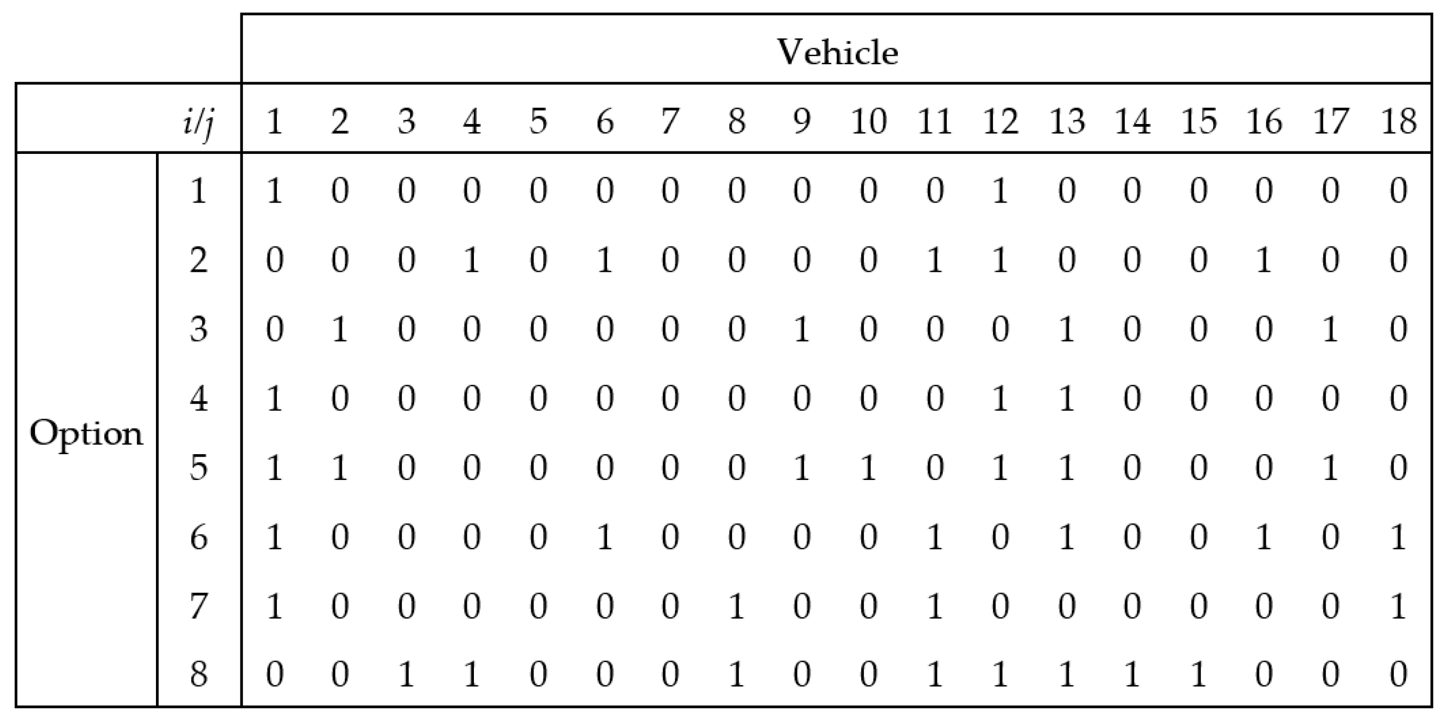
In the sequencing problem, the input data are a set of vehicles to be executed r during a work shift, a set of options for a given version, and constraints 1/q. The set of vehicles to be completed during a work shift includes information about the required options for each vehicle and is determined by the order coordination department (Figure 2).

Figure 2.
The solution representation of the CSP for a set of 18 vehicles, n = 18 and a set of 8 options, m = 8, where 1 means that option i can appear in vehicle version j.
The space of possible solutions in CSP includes all possible permutations of vehicles V, requiring different configurations of options O [15]. CSP is an NP-hard problem, as shown in [14,32]. The proposed methods for solving CSP are based on exact or approximate methods [8,33]. The first group involves systematic exploration of the search space until a solution is found or it is proven that there is no solution. In practical applications, they can be effective in solving cases with low n and are not competitive with heuristic methods [15]. Moreover, in practical problems, in many cases, there is no solution that meets all the constraints, and the decision-making problem comes down to searching for a solution that exceeds them as little as possible. In the group of heuristic methods, the most common are greedy algorithms, local search, genetic algorithms and ant algorithms [15]. In this paper, approaches based on a dedicated greedy algorithm, simulated annealing algorithm, and grey wolf optimizer are proposed to solve the analysed problem.
2.1. The Greedy Algorithm
The greedy algorithm creates a sequence by selecting the best local solution for the current sequence and the first unallocated vehicle with the “heaviest” version. The proposed greedy algorithm GR (Figure 3) was developed for the needs of the planning department of one of the automotive industry companies and served as a basis for comparison in the presented research results. The auxiliary function find_gaps() determines the distance to the nearest product with the oi option for each position in the current sequence S. The algorithm favours constraints for versions which the increase in labour consumption is the highest, i.e., for which the value qj of constraints among vehicles not yet assigned is the highest. In the event that it is not possible to find an item that meets the imposed conditions, the product is allocated in the position furthest from the already-allocated product with the same option.
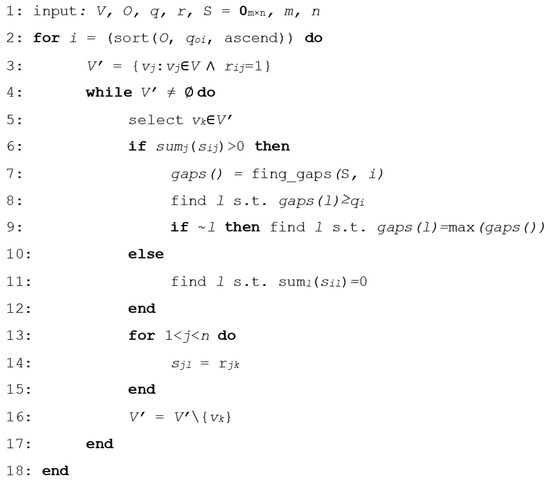
Figure 3.
Steps of the greedy algorithm for the sequencing problem.
The CSP solution is an S matrix whose columns correspond to the vectors of individual vehicle versions. The input data are: a set V of products to be executed, a set O of options that may appear in a given version of the product and the requirements for the option r: V × O ⇒ {0,1}.
2.2. The Simulated Annealing Algorithm
The simulation annealing (SA) heuristics algorithm was proposed by Kirkpatrick et al. [34] and Cerny [35]. The AS algorithm is a stochastic approach and is based on the analogy to the annealing of ideal crystals in thermodynamics and the problem of solving large combinatorial optimization problems [36]. For each temperature change step corresponding to the slow cooling of metals, the SA algorithm probabilistically generates a new potential solution and probabilistically decides between moving the system to the new state or staying in the current state. The algorithm used in this study is a modified version of the standard SA algorithm [37]. The modifications concern protection against staying within the local minimum too long. The number of iterations (70) is determined in which the newly generated solution is adopted, after which the temperature is reset. After each iteration k of the algorithm, the temperature is reduced according to the exponential function t(k) = ti 0.95k. In turn, the probability P(A) of accepting a candidate sequence f(Scnd) worse than the current point f(Scur) is defined in two variants as:
and
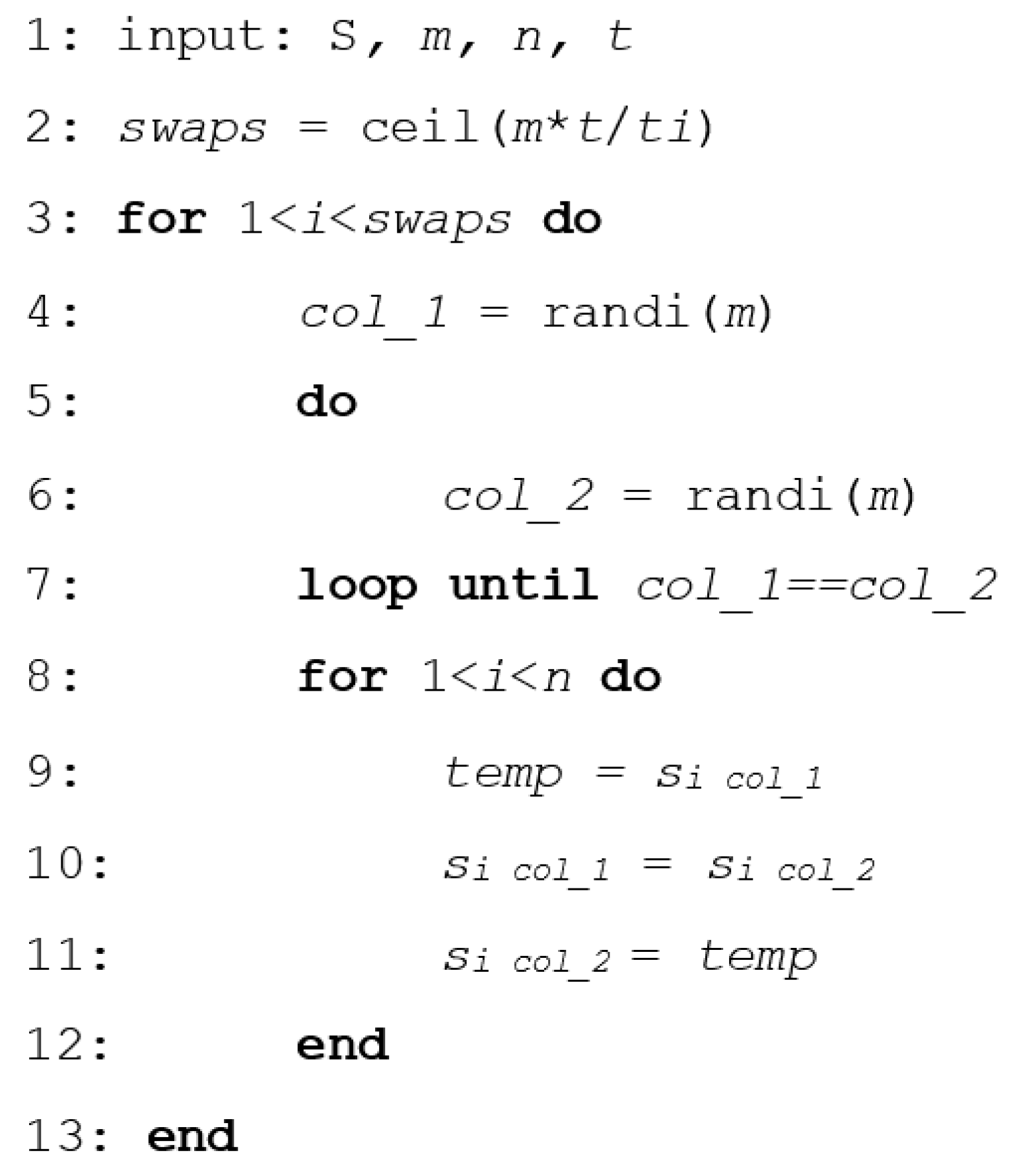
Generating a candidate solution (candidate sequence) is generated by repeatedly replacing two randomly selected columns of matrix S. This multiplicity is variable and corresponds to the product n and the ratio of the current temperature t to the initial temperature ti (Figure 4):

Figure 4.
Steps of the simulated annealing algorithm for the sequencing problem.
The sequences determined as a result of the algorithm execution (for both probability functions) are compared to the random sequence and the base sequence—the sequence obtained as a result of the greedy algorithm.
2.3. The Gray Wolf Optimizer
The grey wolf optimizer GWO is a metaheuristic algorithm proposed by Mirgalili et al. in 2014. GWO imitates the habits of grey wolf packs: the hierarchical stratification and prey behaviour during an attack [38]. A pack contains on average 5 to 12 wolves from four classes with different statuses: alpha(α), beta(β), delta(δ), and omega(ω) wolves. Individual α makes decisions about group actions. The β group assists the α wolves and becomes α when the α wolf dies or gets old. The δ wolf trains the α wolf and reinforces the α wolf’s commands to the lowest level wolves. The ω wolf follows the orders of higher-level wolves to support the tasks they need to complete.
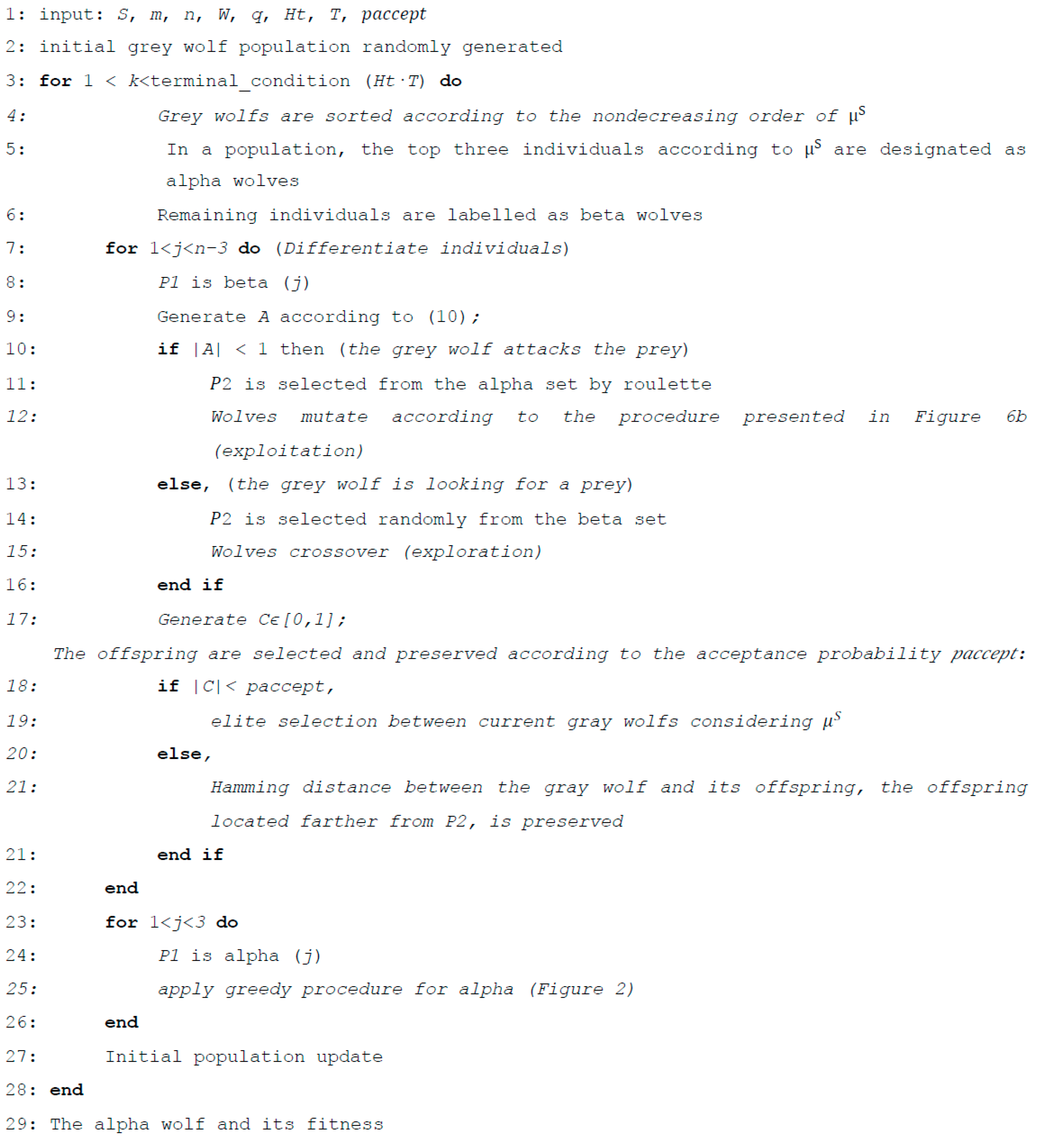
The discrete interpretation of the GWO mathematical model presented in [28] has been modified to apply to the sequencing problem. The GWO architecture is divided into four parts: surrounding, hunting, attacking, and searching for prey. Initially, the three wolf leaders stand as prey positions. The steps of the GWO are presented in Figure 5 for the sequencing problem.
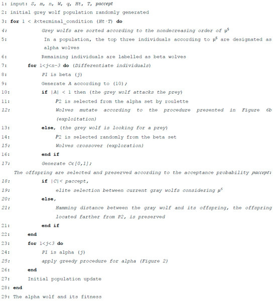
Figure 5.
Steps of the GWO for the sequencing problem.
The initial wolf population is initialized at random. The algorithm is limited to only two populations: alpha and beta wolves. The three best individuals according to (5) in a population are labelled as alpha wolves; the remaining individuals are labelled as beta wolves.
For each beta wolf, Parameter A is generated to decide between exploitation and exploration. When A < 1, the attack procedure is performed, in other words, the solution space is exploited. When A ≥ 1, beta wolves search for a prey, the exploration procedure is applied. Parameter A controls the intensity of global and local search mechanisms of the solution space. When |A| < 1, the beta wolf moves towards the alpha wolf in the population, which means that the algorithm puts emphasizes local search. Otherwise, the beta wolf moves away from the alpha wolf, which means that the algorithm focuses on a global search. Parameter A is generated with a linearly decreasing trend:
where t is the number of current iterations, T is the total number of iterations, and is used to correct the non-linear downward trend of a.
In order to control the exploration and exploitation processes, a non-linear strategy of generating control parameters based on exponential functions from [28] is adopted. In the early iteration of GWO, parameter a is generated with a descent rate that is accelerated to improve the convergence rate of the algorithm. In later iterations, the slowdown is intended to increase the usefulness of GWO. In [28] the convergence trend of parameter a for different values of is presented.
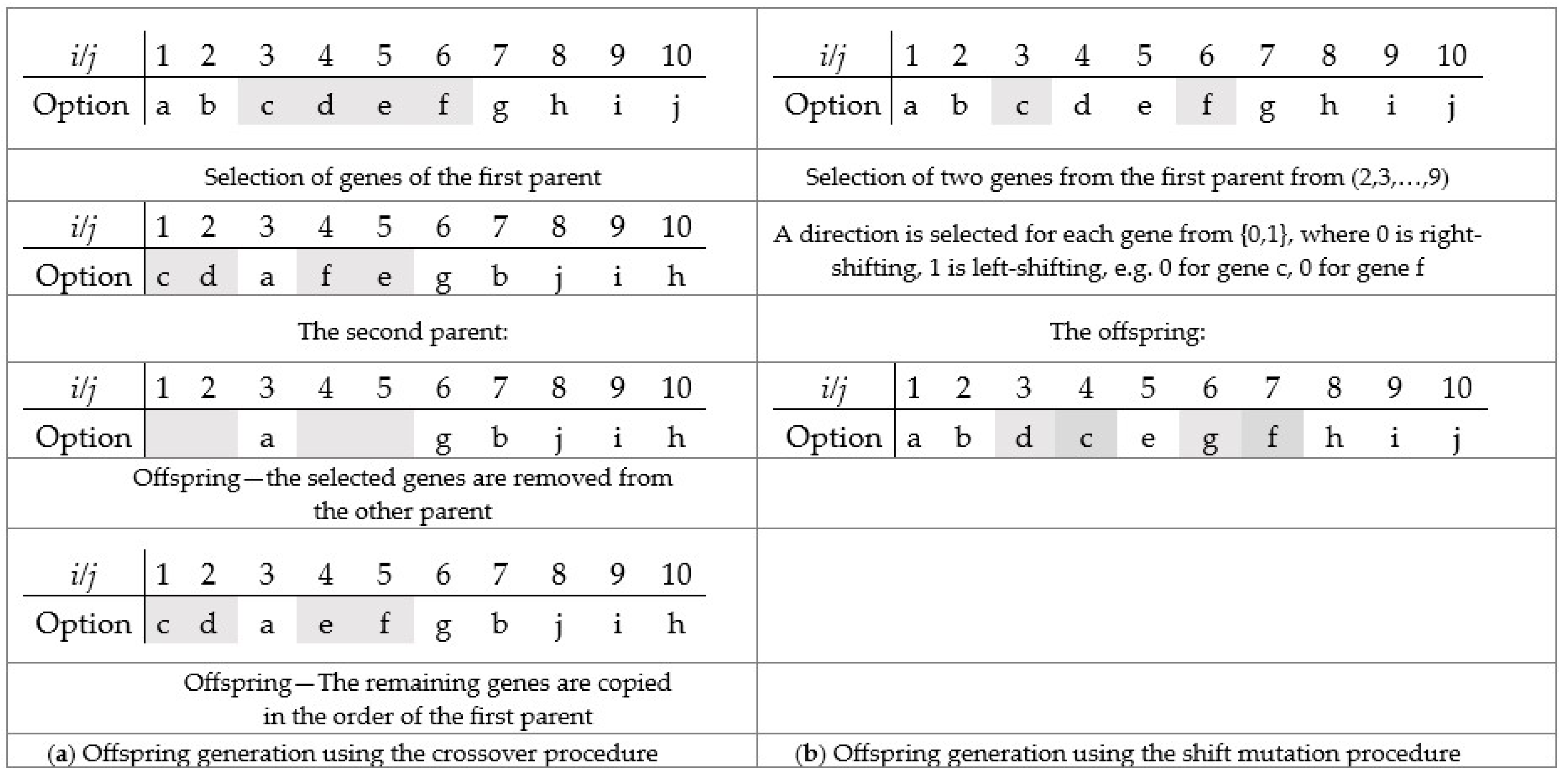
Similarly, for each beta wolf, parameter C is selected to decide between exploitation and exploration. The offspring are selected and preserved according to the acceptance probability paccept. When C < paccept, a close but better solution is probably selected for exploitation. When C ≥ paccept, it is more probable that a distant solution is selected for exploration. The offspring is generated using crossover or mutation procedure. In the crossover procedure (Figure 6a), a subchromosome is randomly selected from the [1, V] range. Selected genes are removed from the other parent’s chromosome. The remaining genes of the second parent are copied in the order of the first parent. In the mutation procedure (Figure 6b), two genes are randomly selected from the range [2, V−1], and the copy direction before or after the mutation point is randomly selected from {0,1}. Offspring are generated using the shift mutation procedure for each selected gene and direction.
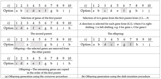
Figure 6.
Crossover (a) and mutation (b) procedure for the car sequencing problem.
Surrounding and hunting is also used with alpha wolves in a greedy procedure. The greedy procedure can also be interpreted as changing the leader of the pack to a new, younger one.
3. Results and Detailed Discussions
The algorithms proposed in the previous chapter were implemented in the MATLAB computing environment. First, computer simulations were carried out for GWO with constraints on generating vehicle versions (9 options), q—constraint vector q = [8 5 6 3 4 4 7 4 8] and the following input data: number of wolves in the pack W = 10; number of hunting trails Ht = 30, = 1.5 (parameter of formula 8); total iteration number in each hunting trail, T = 5; Euler number = exp(1); accept = 0.5.
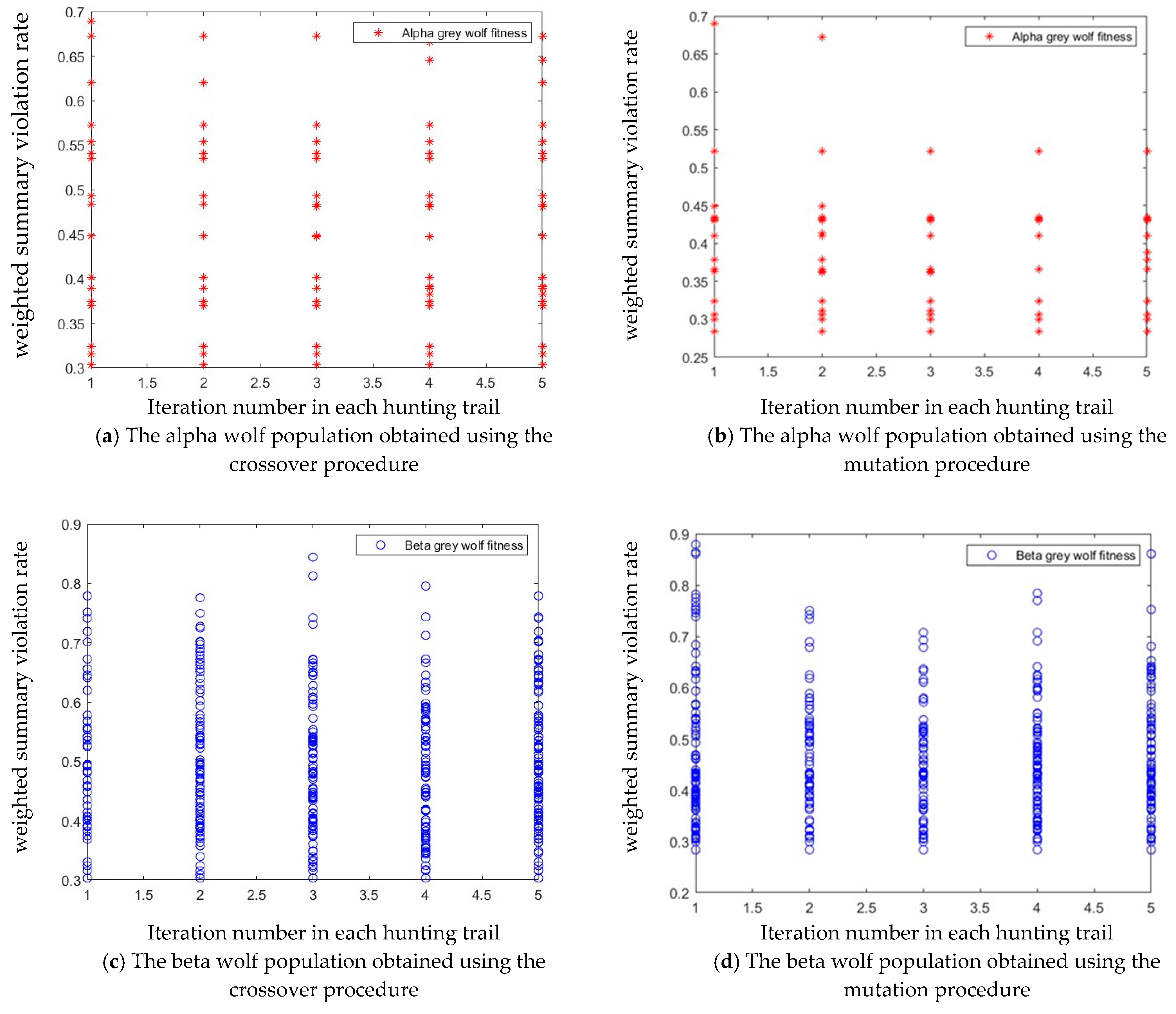
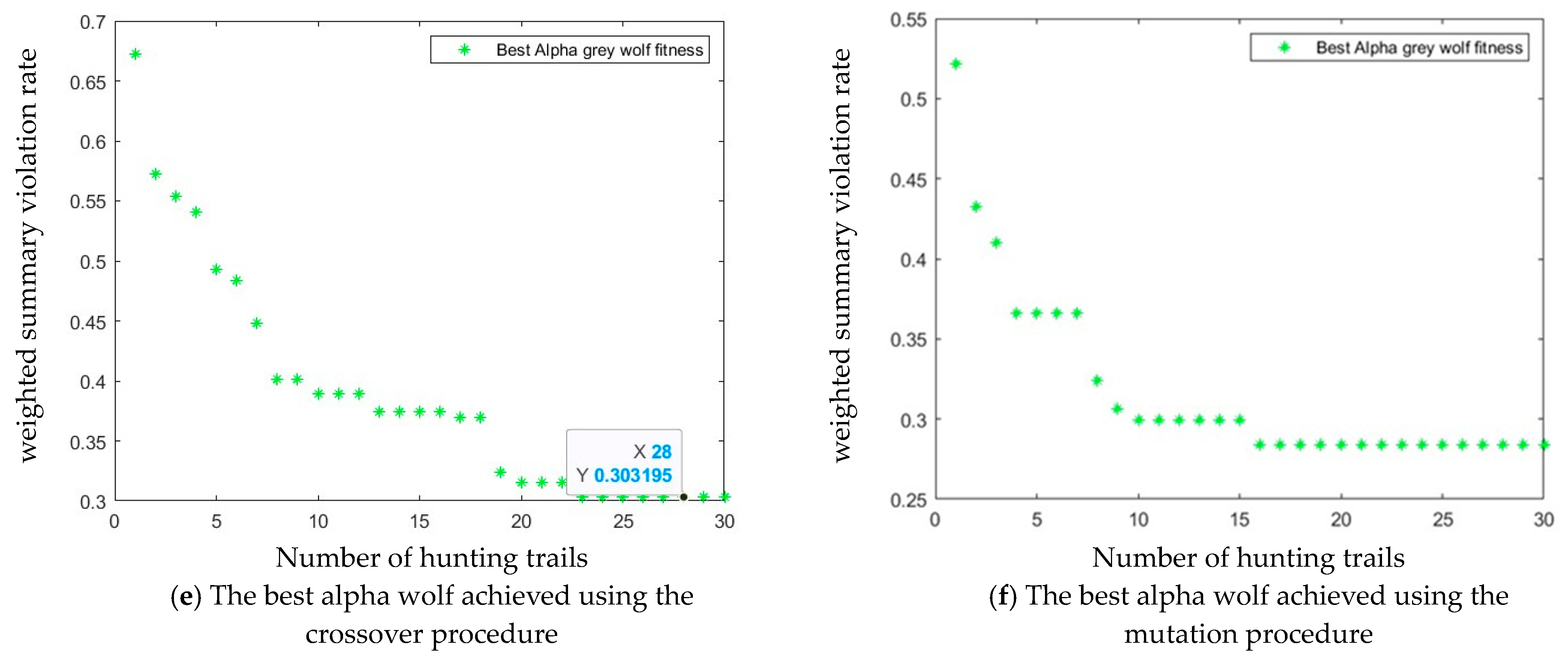
Computer simulations were performed for the GWO using the crossover procedure described in Figure 6a. Figure 7c on the Y-axis shows the fitness function values (5) of the beta wolves achieved in each population (X-axis) in each trail. Similarly, Figure 7a on the Y-axis shows the values of the alpha wolf fitness function. Figure 7e on the Y-axis shows the fitness function values of the best alpha wolf achieved in the last iteration in each trail. The best sequence was achieved for the weighted summary violation rate, = 0.3032 in trails from 23 to 30 (Figure 8a).
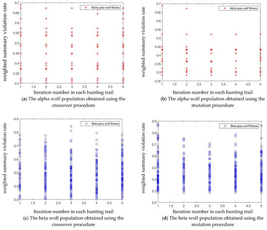
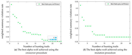
Figure 7.
Population alpha (a,b) and beta (c,d) obtained by computer simulation for input data {W = 10, Ht = 20, = 1.5, T = 5; Euler number = exp(1); accept = 0.5;}. The best alpha wolf (e,f) achieved by the GWO in each hunting trail and each iteration. Populations achieved using crossover (a,c,e) and mutation (b,d,f) procedures.

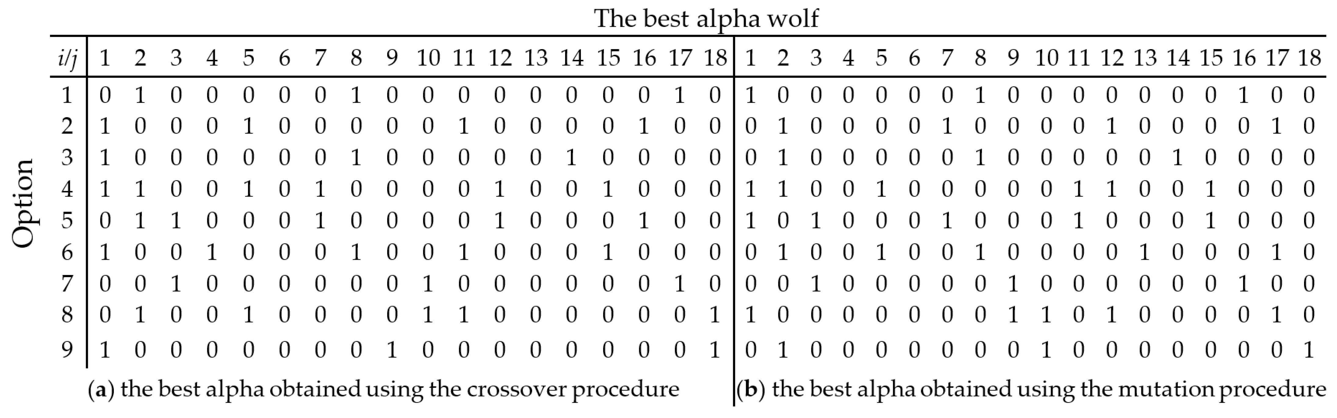
Figure 8.
The best alpha wolf obtained using (a) crossover procedure, (b) mutation procedure for input data {W = 10, Ht = 20, = 1.5, T = 5; Euler number = exp(1); accept = 0.6;}.
The GWO balances the processes of exploration and exploitation because it is able to escape from the local optimum, which can be observed by analysing the best alpha solutions obtained in subsequent hunting trials. Computer simulations were also performed for the GWO using the mutation procedure described in Figure 6b. Results are presented in Figure 7b,d,f. The best sequence was obtained in trails from 16 to 30 for the weighted summary violation rate = 0.2838 (Figure 8b).
The observation and analysis of sensitivity of the GWO performance to changes in “input” parameters of the algorithm can provide information useful for optimizing the sequencing problem. The observation and sensitivity analysis of the GWO are presented in the next section.
3.1. The Influence of Input Parameters on the Weighted Summary Violation Rate
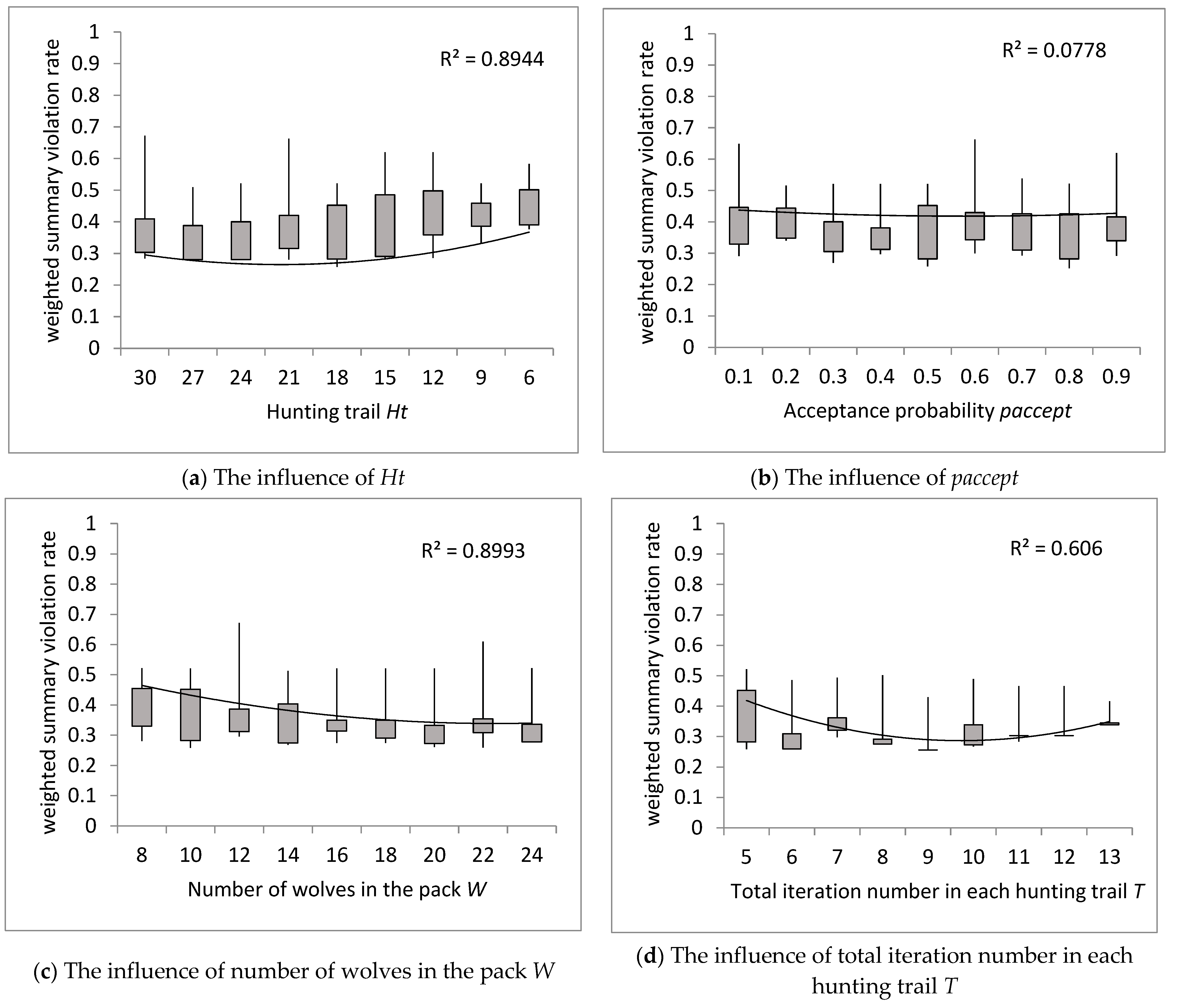
First, we investigated the effect of Ht on the weighted summary violation rate . The weighted summary violation rate decreases with an increase in the number of hunting trails to the minimum value achieved for Ht = 18 and then increases with an increase in the number of trails (Figure 9a). The decreasing and then increasing value of means that is not necessary to achieve the best-quality solution for small and large numbers of hunting trails. The similar conclusion can be drawn for the total iteration number in each hunting trail (Figure 9d).
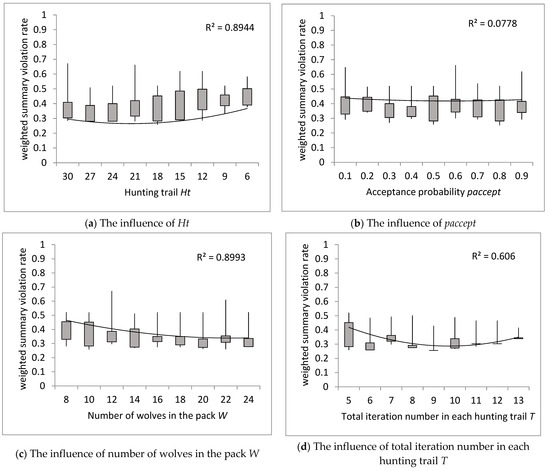
Figure 9.
The influence of changes in input parameters on the weighted summary violation rate: (a) hunting trail Ht, (b) paccept, (c) number of wolves in the pack W, and (d) total iteration number in each hunting trail T.
Offspring are selected and preserved according to their acceptance probability paccept. When C < paccept, a close but better solution is probably to be selected for exploitation. When C ≥ paccept, it is more likely a distant solution will be selected for exploration. The GWO balances exploration and exploitation very well, therefore the effect of paccept is difficult to notice (Figure 9b).
Next, we examine the effect of the number of wolves in the pack W on . The weighted summary violation rate decreases as the number of W increases (Figure 9c). The decreasing value of means that as the number of wolves increases, the chances of achieving a better solution increase.
The best sequence with minimum weighted summary violation rate was achieved for q = [8 5 6 3 4 4 7 4 8] and input data: {W = 10; Ht = 18, = 1.5; T = 5; accept = 0.5}. The best sequence has been improved, = 0.258, compared to the solution presented in Figure 8.
3.2. The Comparative Analysis
Then, the results obtained using the GWO were compared with those obtained using the greedy heuristic and simulated annealing algorithm for both probability functions (6) and (7). The input data includes a set of vehicles to be executed during a work shift, a set of options for a given version and constraints 1/q. The set of vehicles to be completed during a work shift includes information about the required options for each vehicle and is determined by the order coordination department. In order to compare the algorithms, 10 such cases proposed by the Procurement Coordination Unit for sequencing problems of different sizes (m × n) were taken into account (Table 1).

Table 1.
Ten case studies and the solutions generated at random (RAN) using GR and SA with probability function (6) (SA P(A) > 3) and (7) (SA P(A) > 4) and GWO for sequencing problems of different sizes (m × n).
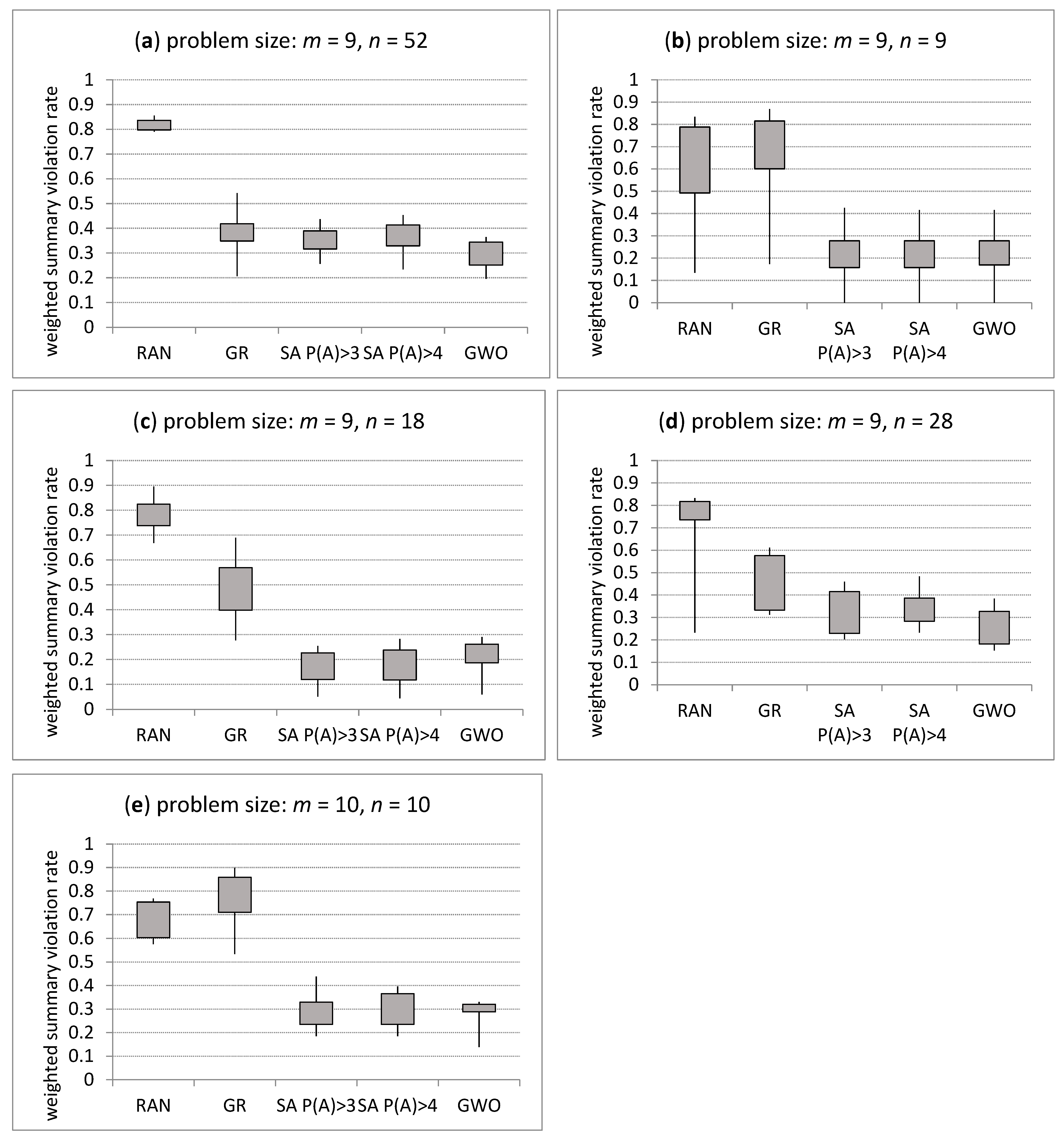
Let us analyse a real car sequencing problem for a set of 52 heavy vehicles and a set of 9 different options that can be present in a given product version (Table 1). Better sequences were obtained using the GWA for the 10 required options proposed by the procurement coordination. The GWO obtained lower weighted summary violation rates than GR, SA P(A) > 3 and SA P(A) > 4. By analysing the minimum, maximum, first quantile, and third quantile of the weighted summary violation rate of obtained solutions (Figure 10a), the following conclusion can be drawn: the GWO outperforms the other algorithms.
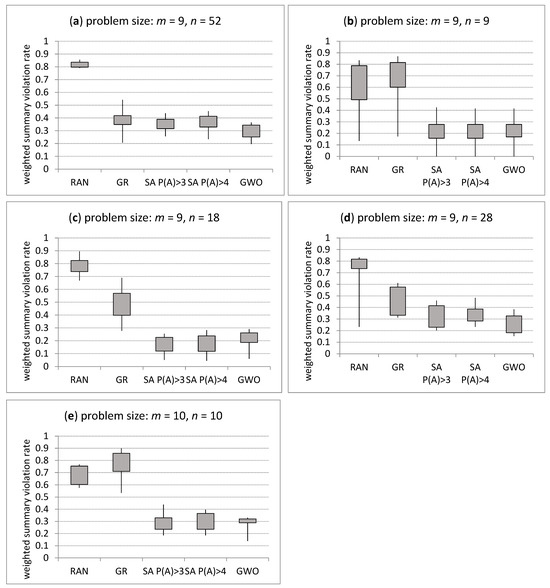
Figure 10.
The solutions generated at random (RAN), using GR, SA with probability function (6) (SA P(A) > 3) and (7) (SA P(A) > 3) and the GWO for problems: (a) m = 9, n = 52, (b) m = 9, n = 9, (c) m = 9, n = 18, (d) m = 9, n = 28 and (e) m = 10, n = 10.
Let us analyse the CSP for a set of nine vehicles and a set of nine different options that can be present in a given product version, n = 9 and m = 9, respectively. Solutions obtained using individual algorithms are presented in Table 1. The same sequences were obtained using the GWA and SA except of the required option {6 6 9 5 8 3 9 3 4}. By analysing the minimum, maximum, first quantile, and third quantile of the weighted summary violation rate of solutions achieved using RAN, GR, SA P(A) > 3, SA P(A) > 4 and the GWO (Figure 10b) for n = 9 and m = 9, the following conclusion can be drawn: the GWO obtained similar solutions to the SA.
Let us analyse the CSP for a set of 18 vehicles and a set of 9 different options that can be present in a given product version (Table 1 and Figure 10c). SA outperforms the GWA.
By analysing the CSP for a set of 28 vehicles and a set of 9 different options that can be present in a given product version (Table 1 and Figure 10d), the opposite conclusion can be drawn: the GWO obtained better solutions than the SA.
Let us analyse the CSP for a set of 10 vehicles and a set of 10 different options that can be present in a given product version (Table 1 and Figure 10e). The best sequence generated by the GWO was achieved for five options {3 3 5 6 8 8 9 9 6}, {6 7 7 5 7 8 7 6 3}, {9 7 3 9 3 9 9 4 9}, {5 7 4 4 4 8 9 3 9}, and {7 5 8 6 6 4 3 8 8}. Additionally, the best sequence generated by SA P(A) > 3 was achieved for five sets of options. The best sequence generated by SA P(A) > 4 was achieved for two sets of options. Thus, the quality of solutions obtained by the GWO and the SA P(A) > 3 is equal.
Overall research performance of the GWO on the sequencing problem is more effective for large-sized sequencing problems.
3.3. Discussion
Thanks to the GWO parameters, A and C, each beta wolf decides between exploitation and exploration. The parameters controlled the intensity of global and local search mechanisms of the solution space. When the beta wolf approaches the alpha wolf in a population, local solutions are sought. When the beta wolf, away from the alpha wolf, survives, a global solution is sought. Making the decision between exploitation and exploration is similar to the decision process in an ant colony optimization (ACO) algorithm [39]. The difference concerns the formulas for the probability of choosing a search strategy. In the ACO, the formulae are based on pheromone parameters, i.e., common intelligence acquired by individuals in previous generations and the quality of the potential solution to the analysed problem. In the GWO, the adaptive convergence factor (8) is used to decide between the global and local search capabilities of the algorithm. At the beginning of the GWA, the local search strategy is promoted. As the number of iterations increases the global search becomes crucial.
The third parameter, the number of hunting trails Ht, makes it possible to exit the local minimum in a situation where a certain number of hunting attempts of the herd have been unsuccessful. In practice, this means giving up hunting for the prey when too much effort is required or when the prey is simply faster.
Offspring are generated via crossover or mutation procedures. Using the crossover procedure, more genetic material is lost than using the mutation procedure. In other words, more distant (different) solutions are generated in the crossover procedure (Figure 6a). In the mutation procedure (Figure 6b), only two genes are randomly selected and shifted. Ultimately, a mutation procedure is applied to generate the offspring in order to preserve the heritage, knowledge, or skills of wolves in the pack.
Observing the results of the sensitivity analysis of the GWO performance to changes in the “input” parameters, the following conclusions can be drawn regarding the optimization of the sequencing problem:
- Decreasing and then increasing the value of μS while increasing Ht means that the number of hunting trails could not be too small or too large to obtain the best quality solution (Figure 9a). A similar conclusion can be drawn for the total number of iterations (hunting attempts on the trail) T, which is closely related to Ht (Figure 9d). When too much energy is spent hunting prey, the grey pack simply gives up.
- The GWO balances exploration and exploitation very well. Thus, the effect of paccept is difficult to notice (Figure 9b).
- The decreasing value of μS as the value of W increases (Figure 9c) indicates that as the number of wolves increases, the chances of achieving a better solution also increase.
After tuning the GWO parameters, the algorithm was compared to the GR and the SA for probability functions (6) and (7). The GWO outperforms the other algorithms in two CSPs, namely (9 × 28) and (9 × 52). The performance of the GWA is better than GR, SA for large size car sequencing problems. Overall research performance of the GWO on the sequencing problem is effective.
4. Conclusions
In the face of the negative effects of climate change, much attention is paid to the issue of greenhouse gas emissions. Following the dynamically accelerating climate and energy trends, transition challenges and strategic decisions are presented in [40]. Companies operating in energy-intensive industries constitute as many as four fifths of companies listed in the steel industry [41]. Reducing energy consumption in car factories will also have a positive impact on reducing greenhouse gas emissions.
Production departments deal with problems of unsynchronized flows resulting from broken supply chains and high energy consumption in transport between different production departments. This article addresses the problem of car sequencing on the assembly line of mixed models. The criteria for assessing the proposed solutions take into account the mixed model production and, indirectly, energy consumption.
The proposed CSP solving algorithms have demonstrated their effectiveness in solving the considered CSP class. The obtained results are better in a significant number of cases than those obtained with greedy algorithms used in industrial practice. They can therefore be successfully implemented in systems supporting assembly sequencing planning, in particular in relation to multi-version and multi-model lines with a large variation in assembly times, e.g., heavy vehicle manufacturers.
The original value of the paper was the development of the grey wolf optimizer for the mixed-model assembly line sequencing problem. The algorithm was selected due to its efficiency in solving scheduling problems [25] compared to other biologically inspired algorithms: smart swarm optimization [26], flame moth optimization algorithm [27], and salp swarm algorithm [28]. Further research will include comparing GWO with other metaheuristic methods in the sequencing tasks of the assembly line with an emphasis on sustainable production.
Author Contributions
Conceptualization, I.P. and D.K.; methodology, D.K and I.P.; software, D.K and I.P.; validation, I.P.; formal analysis, I.P. and D.K.; investigation, I.P. and D.K.; resources, I.P. and D.K.; writing—original draft preparation, I.P. and D.K.; writing—review and editing, I.P. and D.K.; visualization, I.P; supervision, I.P. and D.K; funding acquisition, I.P. All authors have read and agreed to the published version of the manuscript.
Funding
The publication is supported by the rector’s pro-quality grant. Silesian University of Technology, grant number 10/020/RGJ/22/1024.
Data Availability Statement
Not applicable.
Conflicts of Interest
The authors declare no conflict of interest.
References
- Menghi, R.; Papetti, A.; Germani, M.; Marconi, M. Energy efficiency of manufacturing systems: A review of energy assessment methods and tools. J. Clean. Prod. 2019, 240, 118276. [Google Scholar] [CrossRef]
- Renna, P.; Materi, S. A literature review of energy efficiency and sustainability in manufacturing systems. Appl. Sci. 2021, 11, 7366. [Google Scholar] [CrossRef]
- Final Energy Consumption in Industry—Detailed Statistics. Statistics Explained, Eurostat. 2023. Available online: https://ec.europa.eu/eurostat/statistics-explained/index.php?title=Final_energy_consumption_in_industry_-_detailed_statistics (accessed on 25 August 2023).
- The Annual Energy Outlook (AEO2023). U.S. Energy Information Administration. 2023. Available online: https://www.eia.gov/outlooks/aeo/ (accessed on 25 August 2023).
- Use of Energy Explained. Energy Use in Industry. U.S. Energy Information Administration. 2023. Available online: https://www.eia.gov/energyexplained/use-of-energy/industry-in-depth.php (accessed on 25 August 2023).
- Sato, F.E.K.; Nakata, T. Energy Consumption Analysis for Vehicle Production through a Material Flow Approach. Energies 2020, 13, 2396. [Google Scholar] [CrossRef]
- Energy Consumption during Car Production in the EU. The European Automobile Manufacturers’ Association (ACEA). 2023. Available online: https://www.acea.auto/figure/energy-consumption-during-car-production-in-eu/ (accessed on 25 August 2023).
- Boysen, N.; Fliedner, M.; Scholl, A. Sequencing mixed-model assembly lines: Survey, classification and model critique. Eur. J. Oper. Res. 2009, 192, 349–373. [Google Scholar] [CrossRef]
- Liao, M.-L. Construction and comparison of multi-model and mixed-model assembly lines balancing problems with bi-objective. J. Ind. Prod. Eng. 2014, 31, 483–490. [Google Scholar] [CrossRef]
- Gjeldum, N.; Salah, B.; Aljinovic, A.; Khan, S. Utilization of Industry 4.0 Related Equipment in Assembly Line Balancing Procedure. Processes 2020, 8, 864. [Google Scholar] [CrossRef]
- Cohen, Y.; Faccio, M.; Galizia, F.G.; Mora, C.; Pilati, F. Assembly system configuration through Industry 4.0 principles: The expected change in the actual paradigms. IFAC-PapersOnLine 2017, 50, 14958–14963. [Google Scholar] [CrossRef]
- Kim, S.; Jeong, B. Product sequencing problem in Mixed-Model Assembly Line to minimize unfinished works. Comput. Ind. Eng. 2007, 53, 206–214. [Google Scholar] [CrossRef]
- Rahimi-Vahed, A.; Mirzaei, A.H. A hybrid multi-objective shuffled frog-leaping algorithm for a mixed-model assembly line sequencing problem. J. Comput. Ind. Eng. 2007, 53, 642–666. [Google Scholar] [CrossRef]
- Kis, T. On the complexity of the car sequencing problem. Oper. Res. Lett. 2004, 32, 331–335. [Google Scholar] [CrossRef]
- Solnon, C.; Cung, V.D.; Nguyen, A.; Artigues, C. The car sequencing problem: Overview of state-of-the-art methods and industrial case-study of the ROADEF’2005 challenge problem. Eur. J. Oper. Res. 2008, 191, 912–927. [Google Scholar] [CrossRef]
- Bänsch, K.; Busse, J.; Meisel, F.; Rieck, J.; Scholz, S.; Volling, T.; Wichmann, M.G. Energy-Aware Decision Support Models in Production Environments: A Systematic Literature Review. Comput. Ind. Eng. 2012, 159, 107456. [Google Scholar] [CrossRef]
- Lamy, D.; Delorme, X.; Gianessi, P. Line Balancing and Sequencing for Peak Power Minimization. IFAC-PapersOnLine 2020, 53, 10411–10416. [Google Scholar] [CrossRef]
- Zhang, B.; Xu, L.; Zhang, J. A multi-objective cellular genetic Algorithm for energy-oriented balancing and sequencing problem of mixed-model assembly line. J. Clean. Prod. 2019, 244, 118845. [Google Scholar] [CrossRef]
- Wu, J.; Ding, Y.; Shi, L. Mathematical modeling and heuristic approaches for a multi-stage car sequencing problem. Comput. Oper. Res. 2012, 152, 107008. [Google Scholar] [CrossRef]
- Coreau, J.-F.; Laporte, G.; Pasin, F. Iterated tabu search for the car sequencing problem. Eur. J. Oper. Res. 2008, 191, 945–956. [Google Scholar] [CrossRef]
- Briant, O.; Naddef, D.; Mounie, G. Greedy approach and multi-criteria simulated annealing for the car sequencing problem. Eur. J. Oper. Res. 2008, 191, 993–1003. [Google Scholar] [CrossRef]
- Moya, I.; Chica, M.; Bautista, J. Constructive metaheuristics for solving the Car Sequencing Problem under uncertain partial demand. Comput. Ind. Eng. 2019, 137, 106048. [Google Scholar] [CrossRef]
- Ko, S.-S.; Han, Y.-H.; Choi, J. Paint batching problem on M-to-1 conveyor systems. Comput. Oper. Res. 2016, 74, 118–126. [Google Scholar] [CrossRef]
- Zhang, H.; Ding, W. A Decomposition Algorithm for Dynamic Car Sequencing Problems with Buffers. Appl. Sci. 2023, 13, 7336. [Google Scholar] [CrossRef]
- Kennedy, J.; Eberhart, R. Particle swarm optimization. In Proceedings of the ICNN’95-International Conference on Neural Networks, Perth, WA, Australia, 27 November–1 December 1995; pp. 1942–1948. [Google Scholar]
- Mirjalili, S. Moth-flame optimization algorithm: A novel nature-inspired heuristic paradigm. Knowl.-Based Syst. 2015, 89, 228–249. [Google Scholar] [CrossRef]
- Mirjalili, S.; Gandomi, A.H.; Mirjalili, S.Z.; Saremi, S.; Faris, H.; Mirjalili, S.M. Salp Swarm Algorithm: A bio-inspired optimizer for engineering design problems. Adv. Eng. Softw. 2017, 114, 163–191. [Google Scholar] [CrossRef]
- Kong, X.; Yao, Y.; Yang, W.; Yang, Z.; Su, J. Solving the Flexible Job Shop Scheduling Problem Using a Discrete Improved Grey Wolf Optimization Algorithm. Machines 2022, 10, 1100. [Google Scholar] [CrossRef]
- Chen, R.H.; Yang, B.; Li, S.; Wang, S.L. A self-learning genetic algorithm based on reinforcement learning for flexible job-shop scheduling problem. Comput. Ind. Eng. 2020, 149, 106778. [Google Scholar] [CrossRef]
- Gravel, M.; Gagné, C.; Price, W.L. Review and comparison of three methods for the solution of the car sequencing problem. J. Oper. Res. Soc. 2005, 56, 1287–1295. [Google Scholar] [CrossRef]
- Parrello, B.; Kabat, W.; Wos, L. Job-shop scheduling using automated reasoning: A case study of the car-sequencing problem. J. Autom. Reason. 1986, 2, 1–42. [Google Scholar] [CrossRef]
- Gent, I.P. Two Results on Car Sequencing Problems; Technical Report APES APES-02; University of Strathclyde: Glasgow, UK, 1998. [Google Scholar]
- Chutima, P.; Olarnviwatchai, S. A multi-objective car sequencing problem on two-sided assembly lines. J. Intell. Manuf. 2018, 29, 1617–1636. [Google Scholar] [CrossRef]
- Kirkpatrick, S.; Gelatt, C.D., Jr.; Vecchi, M.P. Optimization by simulated annealing. Science 1983, 220, 671–680. [Google Scholar] [CrossRef]
- Černý, V. Thermodynamical approach to the traveling salesman problem: An efficient simulation algorithm. J. Optim. Theory Appl. 1985, 45, 41–51. [Google Scholar] [CrossRef]
- van Laarhoven, P.J.M.; Aarts, E.H.L. Simulated annealing. In Simulated Annealing: Theory and Applications. Mathematics and Its Applications; Springer: Dordrecht, The Netherlands, 1987; Volume 37. [Google Scholar]
- Eglese, R.W. Simulated annealing: A tool for operational research. Eur. J. Oper. Res. 1990, 46, 271–281. [Google Scholar] [CrossRef]
- Mirjalili, S.; Mirjalili, S.M.; Lewis, A. Grey Wolf Optimizer. Adv. Eng. Softw. 2014, 69, 46–61. [Google Scholar] [CrossRef]
- Paprocka, I.; Krenczyk, D.; Burduk, A. The method of production scheduling with uncertainties using the ants colony optimization. Appl. Sci. 2021, 11, 171. [Google Scholar] [CrossRef]
- Energy Policy of Poland until 2040 (EPP2040). Available online: https://www.gov.pl/web/climate/energy-policy-of-poland-until-2040-epp2040 (accessed on 25 August 2023).
- Chen, J.; Sun, C.; Wang, Y.; Liu, J.; Zhou, P. Carbon emission reduction policy with privatization in an oligopoly model. Environ. Sci. Pollut. Res. Int. 2023, 30, 45209–45230. [Google Scholar] [CrossRef] [PubMed]

Disclaimer/Publisher’s Note: The statements, opinions and data contained in all publications are solely those of the individual author(s) and contributor(s) and not of MDPI and/or the editor(s). MDPI and/or the editor(s) disclaim responsibility for any injury to people or property resulting from any ideas, methods, instructions or products referred to in the content. |
© 2023 by the authors. Licensee MDPI, Basel, Switzerland. This article is an open access article distributed under the terms and conditions of the Creative Commons Attribution (CC BY) license (https://creativecommons.org/licenses/by/4.0/).