Abstract
The electric capacitance tomography (ECT) technique has been widely used in phase distribution reconstruction, while the practical application raised nonideal noise and other errors for cryogenic conditions, requiring a more accurate algorithm. This paper develops a new image reconstruction algorithm for ECT by coupling the traditional Landweber algorithm with the least square support vector regression (LSSVR) for cryogenic fluids. The performance of the algorithm is quantitatively evaluated by comparing the inversion images with the experimental results for both the room temperature working medium with the dielectric constant ratio close to cryogenic fluid and the cryogenic fluid of liquid nitrogen/nitrogen vapor (LN2-VN2). The inversion images based on the conventional LBP and Landweber algorithms are also presented for comparison. The benefits and drawbacks of the developed algorithms are revealed and discussed, according to the results. It is demonstrated that the correlated coefficients of the images based on the developed algorithm reach more than 0.88 and a maximum of 0.975. In addition, the minimum void fraction error of the algorithm is reduced to 0.534%, which indicates the significant optimization of the LSSVR coupled method over the Landweber algorithm.
1. Introduction
The occurrence of gas–liquid two-phase flow is prevalent in cryogenic fluid machinery [1], including transfer pipes, heat exchangers, evaporators, and condensers. Therefore, the determination of the phase distribution, which is one of the most vital parameters to classify the two-phase flow, as well as the void fraction, is essential to the cryogenic fluid industry [2,3]. Nevertheless, it is still intractable to measure the phase distribution of cryogenic fluids, either because of the fluid properties or the working conditions [4].
Many efforts have been made to obtain the phase distribution of the cryogenic two-phase flow, including the use of the capacitive probe method [5], the radio-frequency sensor (RF-sensor) [6,7,8], the dual-electrode capacitance sensor [4], and particle image velocimetry (PIV) [9]. Comparably, electrical capacitance tomography (ECT), as a non-intrusive measurement technique, can reconstruct the phase distribution image based on the dielectric permittivity difference between the phases. It also has the advantages of easy assembling, fast imaging, and low cost. Therefore, many studies have been made on its application to image reconstruction for room temperature fluids, such as in fluidized beds [10,11], water/oil flows [12], gas/oil flows [13,14,15,16], and other multi-phase conditions [17,18].
There are few published experimental studies about ECT applied to the cryogenic two-phase flow. The difficulties come from the fact that the dielectric permittivity ratio of the cryogenic liquid to its vapor is usually an order of magnitude smaller than those of the room temperature fluid pair, such as water/air (77.747/1.0005), while the LN2/VN2 (1.4337/1.0021) is much lower [19]. Therefore, the micro-capacitance acquisition circuit is required to have a higher sensitivity and anti-noise interference ability. In our previous studies, the potential feasibility of cryogenic ECT was evaluated [20] by conducting a substitutive ambient temperature experiment based on the pair of materials with a dielectric constant ratio close to that of cryogenic fluids. In addition, the reconstruction algorithm was especially improved to reconstruct the two-phase images for better quality. The potential application of electrical capacitance volume tomography (ECVT) to cryogenic cases was also evaluated by us, using numerical experiments [21], in which the essential roles of the shifted plane and the axial guard electrode play in ECVT were verified. Recently, Hunt et al. [22] conducted a pioneering cryogenic experiment to measure the density of the LN2-VN2 flow based on the eight-electrode ECT system. The ECT sensor in their alternative experiment can provide images of non-conducting inclusions in the flow, representing gas bubbles at room temperature. Although the final LN2-VN2 phase distribution reconstruction image was not obtained, their work was still constructive and provided evidence for the application of ECT in cryogenic fluids. Sun et al. [23] conducted a real-time cross-sectional holdup imaging experiment of high-pressure gas–liquid carbon dioxide (CO2) flow using the ECT method. The accuracy of real-time measurement based on the ECT system was acceptable; it was calculated by three widely used algorithms and evaluated with the images captured at the sight window. The convenience of the Calderon algorithm for the CO2 two-phase image reconstruction was also summarized. Tian et al. [24] compared the performance of deep neural network (DNN) modification to the classical linear algorithms (DNN-EC) and the DNN directly for image reconstruction (DNN-C). The generalization ability of these methods was validated in the numerical experiment, and the feasibility of these models for the cryogenic application was evaluated by a cryogenic experiment. The results showed that the DNN-C is a better solution than the DNN-EC, based on error capacitance. Gao [25] introduced the transformer technique to the U-net convolutional neural network (CNN). The trained CNN was applied to the numerical experiment and achieved excellent and stable results. The model was also used to reconstruct the LN2-VN2 flow in the cryogenic experiment, with clear and accurate images.
The image reconstruction of ECT is a typical underdetermined inverse problem [26] The phase information in the thousands of grid cells of the computational domain is calculated based on a very finite number of measured capacitance values—for example, eight for the eight-electrode ECT. Therefore, the reconstruction algorithm theoretically plays a crucial role in tomography, especially for cryogenic fluids that have a much smaller dielectric constant ratio of liquid to vapor. At present, there are several algorithms widely applied in the ECT image reconstruction developed for room-temperature fluids, including the linear back projection (LBP) [27], the Landweber iteration [28], and the total variation L1-norm regularization (TV L1-norm) [29] algorithms. Many efforts have also been made to improve the algorithms’ efficiencies. Xie et al. [27] demonstrated the significantly increased imaging speed of the back projection algorithm in determining the oil concentration. Yang et al. [28] proposed a new image inversion algorithm based on the modified Landweber iteration algorithm by applying a regularization, which showed a faster convergence speed and enhanced immunity to noise. Liu et al. [30] optimized the iterative step length of the Landweber algorithm based on minimizing the norm of the capacitance error vector. Soleimani and Lionheart [29] employed regularization techniques to overcome the ill-posedness, which proved the advantage of the TV regularization algorithm over the image reconstruction of different inclusions. To enhance the performance of the reconstruction image, Wang et al. [31] proposed an adaptive cell refinement approach based on the TV method to preserve the edge. Li and Yang [19] proposed a nonlinear iteration algorithm, in which the sensitivity matrix was updated rather than fixed in the iterative process. The results indicated that the relative capacitance residual and the image error decrease more quickly than in the fixed sensitivity matrix cases. Guo et al. [11] developed a machine-learning method by avoiding the postprocessing steps, which increased the imaging speed. The training samples were collected in different flow patterns through high-throughput experiments. Xie et al. [20] proposed an approach of the least squares support vector regression (LSSVR) coupled linear algorithm, reducing the error by 68%, at most, via fitting the correlation between the capacitance vector and the linearization error.
In this paper, the least square support vector regression (LSSVR) method was applied to improve the performance of the Landweber algorithm by introducing the sensitivity linear error matrix, which was realized by fitting the relationship between the normalized capacitance vector and the nonlinear error using the training samples. The image reconstruction results, based on the new algorithm together with the LBP algorithm and the original Landweber algorithm, were presented and compared with the experimental observations. A room-temperature experiment with a fluid pair having an electrical dielectric ratio of about 5 was first performed, which indicated the potential of the LSSVR modifying algorithm applied to the small electrical dielectric ratio cases. Then, a visual cryogenic experiment of LN2-VN2 two-phase flow was carried out to further evaluate the reconstructed images of the three algorithms for the eight-electrode ECT. By comparing the cryogenic imaging results of the proposed algorithm with the LBP algorithm and the original Landweber algorithm, it was proved that the proposed algorithm can improve the imaging performance.
2. ECT Cryogenic Experimental System
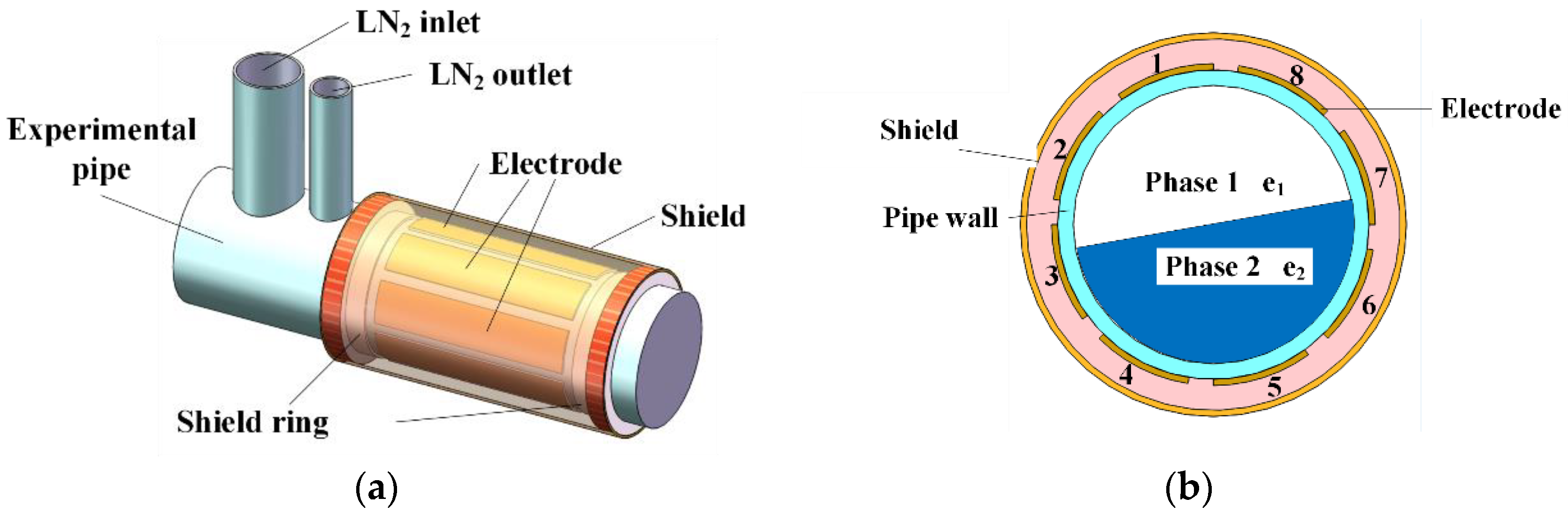
The ECT system for cryogenic flow primarily consists of the eight-electrode sensor, the micro-capacitance acquisition circuit, and the image reconstruction computer with the capacitance tomography algorithm. Figure 1 and Figure 2, respectively, show the scheme and real layout of the ECT cryogenic experiment system. Figure 3 provides the detailed test structure, as well as the cross-section of the sensor.
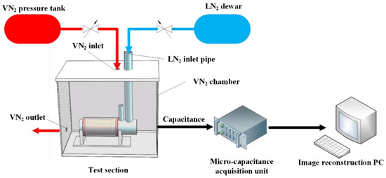
Figure 1.
Scheme of cryogenic ECT experiment system.
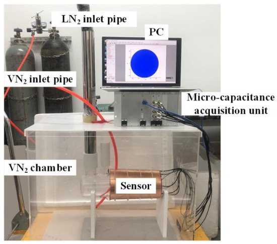
Figure 2.
Cryogenic ECT experimental facility.
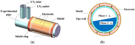
Figure 3.
Cryogenic ECT sensor: overall structure of test section (a) and the cross-section (b).
The sensor primarily comprises the experimental pipe and the eight electrodes uniformly attached to the external surface of the pipe in the circumferential direction. Each electrode has a length of 120 mm parallel to the central axis of the experimental pipe, a circumferential angle of 36°, and a thickness of 0.15 mm; thus, the covering ratio of the electrodes is 80%. The experimental pipe is made of quartz glass with a relative dielectric permittivity of 3.8. It has an outer diameter of 102 mm and a thickness of 2 mm. There is an inlet tube connected for adding the LN2 and another tube for releasing the VN2. Two additional axial shield rings are placed at both ends of the electrodes. Around the electrodes, there exists an electromagnetic shield to avoid the interference of the environmental magnetic field. Both the external and axial shields can reduce the parasitic effect. The material of all the electrodes and shields is copper. The whole cryogenic sensor is placed in a square chamber made of acrylic boards, as shown in Figure 2. The chamber is filled with static nitrogen to replace the original wet air to avoid frosting on the surface of the cryogenic pipe. The nitrogen also serves to reduce the heat leak due to the smaller thermal conductivity compared with the wet air. The design greatly simplifies the facility structure which should be in the complex vacuum insulation, while keeping it visual and maintaining an acceptable heat-leakage rate.
The micro-capacitance acquisition circuit collects the capacitance values between electrodes and transmits them to the computer. It has a signal-to-noise ratio of 60 dB and a measurement accuracy of 0.1 fF. The available total effective capacitance number M from the eight electrodes is 28. The reconstruction computer processes the acquired capacitance data based on the different imaging algorithms and presents the final phase distribution images.
First, the experimental tube was filled with LN2 and VN2 successively to calibrate the sensor. The stratified flows with different liquid levels were obtained when the LN2 slowly evaporated in the pipe, which was filled with LN2 at the beginning. The phase interface can be considered as the steady state because the change of liquid level caused by the evaporation is slow enough. The real phase distributions were recorded by a camera and the capacitance values between different electrodes were collected by the acquisition circuit.
3. Image Reconstruction Approach
3.1. Forward Problem of ECT
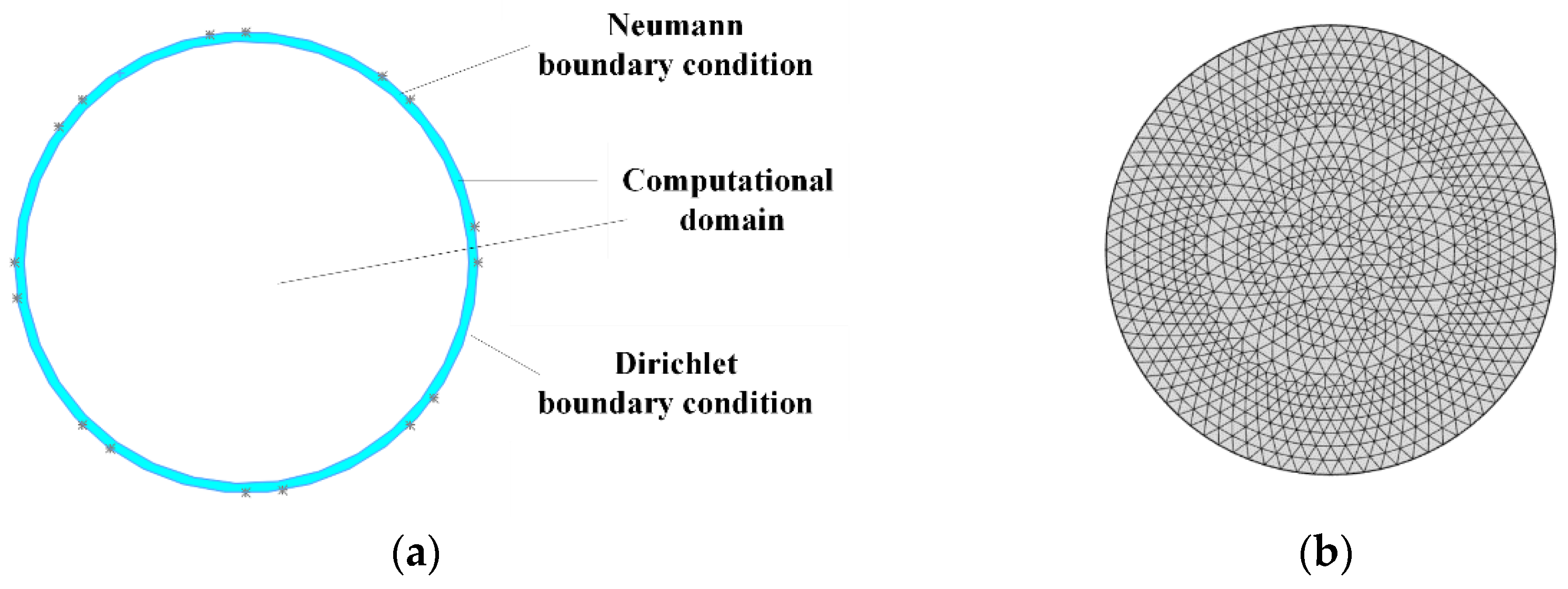
In our previous research, the forward and inverse problem of ECT was illustrated [19], and a brief introduction is presented here. Ignoring the electrode and shield shell, the imaging domain and tube wall are modeled, as shown in Figure 4a. In the calculation, the number N of grid cells in the computational domain is 1836, as shown in Figure 4b.
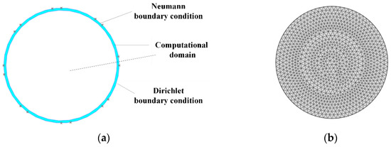
Figure 4.
Computational domain: boundary conditions (a) and grid cell scheme (b).
Because of the characteristics of both the non-polar insulators of LN2-VN2 and the experimental pipe, there is no electronic conduction between the outer environment and the test section. The governing equation of the potential in the computational domain can be obtained as in [32]:
and represent the dielectric permittivity and potential distribution inside the computational domain, respectively.
The boundary conditions are applied according to the actual use process: when electrode i is excited with the voltage , the potential at electrode i is . Meanwhile, when electrode j is grounded, the potential electrode j is 0. Thus, Dirichlet and Neumann boundary conditions are obtained. The total boundary conditions can be written as
In Equation (2), i and j represent the number of electrodes. Γ represents the positions where electrodes exist. Ω represents the computational domain. represents the boundary of the computational domain. represents the boundary of the computational domain which is not covered by the electrodes, and is the unit normal vector outside, toward the wall of the pipe.
When the dielectric permittivity distribution is known, Equation (1) coupled with Equation (2) has a unique solution. This calculation process is the solution to a forward problem [33]. The introduction of will simplify the formula derivation.
where and are the potential distribution in the computational domain when the i and j electrodes are excited by and voltage, respectively, and the other electrodes maintain 0 potential. is the induced charge on electrode i caused by electrode j.
On the other hand, when combined with Equation (1),
Combining Equation (3) with Equation (4), the calculation formula of the mutual capacitance of every electrode pair can be calculated as
3.2. Calculation of Sensitivity Field
The purpose of solving the ECT inverse problem is to find a method to calculate the distribution of dielectric permittivity in the computational domain after measuring the capacitance values of measuring electrode pairs.
For the cryogenic fluid medium, the difference between the liquid and gas dielectric permittivity is relatively small, as shown in Table 1. The slope of the capacitance-dielectric distribution function at the gas phase reference state can be considered to represent the sensitivity [34]. This method can reduce the computational load compared with the conventional ones [27,35], which is widely used in the analysis of capacitive tomography sensors with a liquid–gas dielectric ratio larger than 2.0 in the room-temperature fluid pair [26,34,36].

Table 1.
Relative permittivity of different fluids at 1 atm [19,37].
The computational domain is discretized and the mutual capacitance can be calculated as
where is the dielectric permittivity in each grid cell and represents the dielectric permittivity when all grid cells in the domain are in the gas phase. represents the capacitance between the measurement electrodes i and j when the measurement area is all in the gas phase. represents the second and higher-order terms. is the sensitivity of each grid cell corresponding to the measurement electrodes, which is defined as
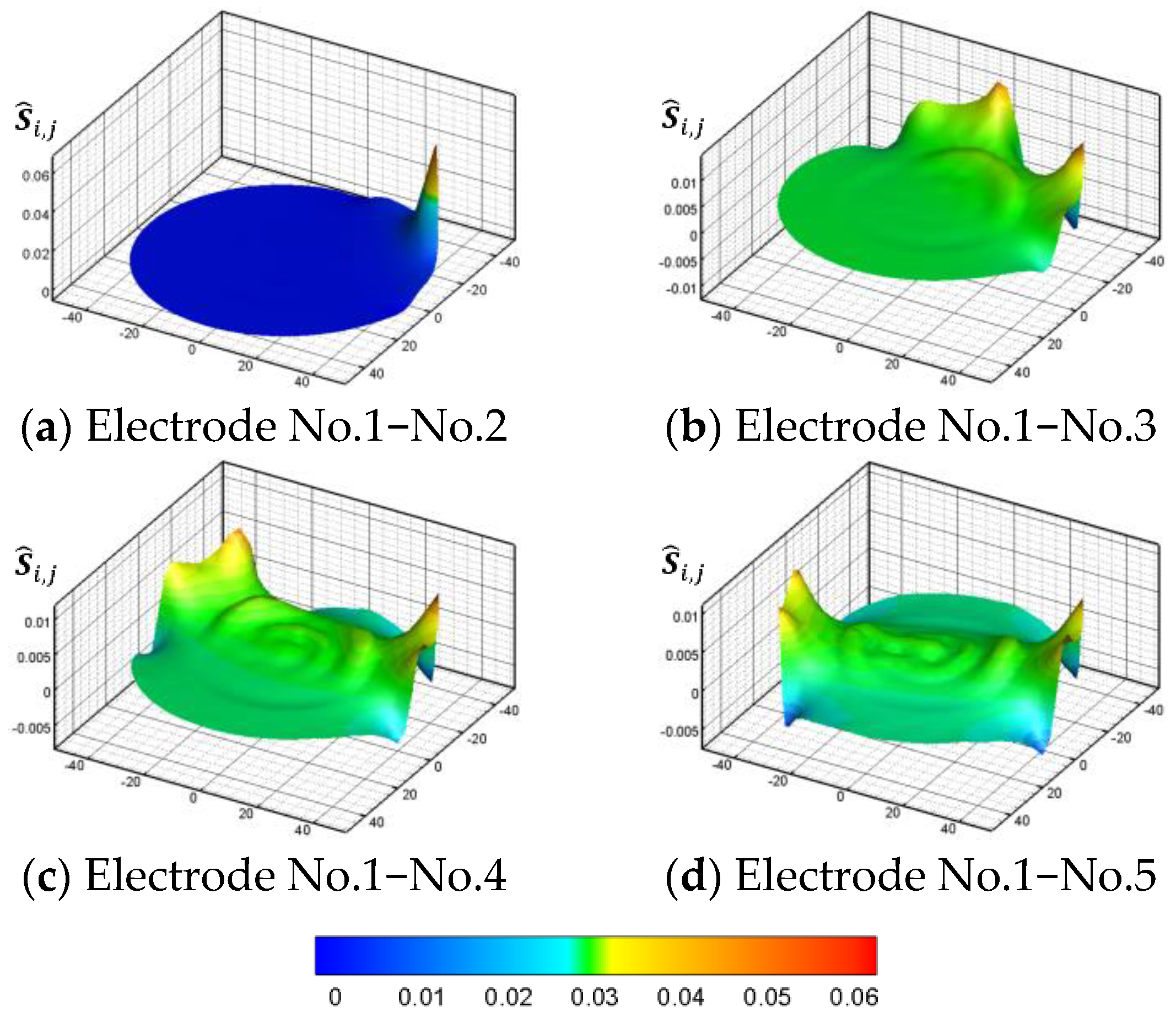
represents the rate of change of the capacitance value to the permittivity of each grid cell. Since there are 28 effective and independent capacitance values, there are 28 independent sensitive fields. The calculation result of the sensitivity field for LN2-VN2 cases is shown in Figure 5. The full 28 sensitivities can be determined from the presented four cases by the relative position of the electrode pair. Since the electrodes of the sensor are centrally symmetric, the 28 sensitive fields can be regarded as a transformation of these four sensitivity fields obtained by rotating 45, 90, 135, or 180 degrees around the center of the measurement area.
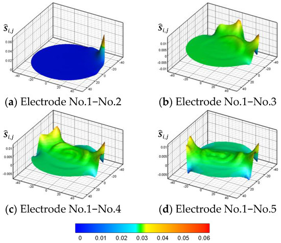
Figure 5.
Sensitivity fields of the corresponding electrode pairs.
It can be found that the sensitivity field in the measurement area is extremely uneven, and the sensitivity reaches the peak at the edge of the electrode. However, from the center of the electrode to the center of the measurement area, the sensitivity changes little and the absolute size is also small.
3.3. The Inverse Problem of ECT
The multi-electrode ECT obtains the dielectric permittivity distribution as well as phase distribution from the measured capacitance data. However, the number N of required phase information in each grid cell is orders of magnitude larger than the number M of measured independent capacitance values. The algorithms of information reconstruction can find a reasonable solution to an underdetermined inverse problem and the different reconstruction algorithms will generate different calculation models.
3.3.1. Linear Back-Projection (LBP) Algorithm
The normalized relationship of measuring capacitance, sensitive field, and dielectric constant is established [27] as
is an normalized sensitivity matrix. is an normalized dielectric permittivity distribution vector which is the acquired result of the inverse problem. The result of the inverse problem is , reflecting the dielectric permittivity of each grid cell relative to the permittivity of the gas phase in the form of gray values. is an normalized measured capacitance vector.
where . P(·) represents the projection operator. The projection operation is carried out on the results [38,39] as the normalization.
Equation (9) is called the projected LBP algorithm, which is the LBP algorithm method applied to this experiment. LBP is applied to the earliest and most widely used ECT inversion algorithm, with the fastest computing speed among all the algorithms. Because there are no iteration steps, the accuracy of the inversion result of the income is relatively low. The result of the LBP algorithm is commonly used for coarse imaging and the iterative initial value of the iterative algorithm.
3.3.2. Landweber Iterative Algorithm
The Landweber iterative algorithm [26] is developed based on the steepest descent method. Consider an unconstrained optimization problem,
Thus, a projected iterative expression can be obtained in the direction of the inverse gradient:
where is the optimal iteration step size of step k [30].
Equation (11) is the Landweber iteration method applied to this experiment. The Landweber iteration with the best iteration step length can achieve a faster convergence rate with higher accuracy of inversion results compared with the ones of the LBP algorithm.
3.3.3. Landweber Coupled LSSVR Algorithm
According to Equation (6), the sensitivity matrix in Equation (7) is a simplified linear model that ignores the higher-order nonlinear information of the electric field. The LSSVR method can fit the relationship between the nonlinear information vector and the measured capacitance vector, based on the provided training set of real phase distribution and the capacitance vector calculated in the forward problem.
The LSSVR maps the low-dimensional sample space into a high-dimensional feature space. Then, the relationship between inputs and outputs is simply fitted through a linear regression equation in a regression hyperplane. Compared with the general support vector regression, the LSSVR solves a linear system of equations by reforming the inequality constraints into minimizing the sum of residual squares. The process of obtaining sensitivity error based on LSSVR is as follows.
The nonlinear error vector is first calculated in each training sample pair.
Here, is an training set matrix of real phase distribution and n is the number of training samples in the training set. is an training set matrix of the normalized capacitance values calculated in the forward problem corresponding to each training sample of real phase distribution. is an nonlinear error matrix calculated by the input phase distribution matrix and capacitance matrix. For the new input of measured capacitance vector E, the nonlinear error vector Y can be obtained using the LSSVR fitting equation:
where is an linear offset vector, is an coefficient vector to map every training sample into the fitting hyperplane, and is the kernel function to map the sample point into the high-dimensional feature space. A mixture kernel function [40] is applied to the LSSVR in this paper, which consists of the Gaussian radial basis function (RBF) kernel function and the polynomial kernel function.
where , , .
The offset vector and the coefficient vector can be obtained by solving the following equation:
,
According to Equations (13) and (14), Equation (11) can be modified as
Equation (16) is the iteration equation of the Landweber coupled LSSVR algorithm. The parameters set for the algorithms are presented in Table 2.
Table 2.
Parameter setting of Landweber algorithm and Landweber coupled LSSVR algorithm.
4. Experiment and Analysis
4.1. The Tentative Experiments
A tentative experiment at the ambient temperature is first conducted to evaluate the reconstruction results of ECT with the above-mentioned algorithms. Figure 6 provides a photo of the ECT system developed by the authors, including the eight-electrode sensor, the electrical capacitance acquisition circuit, and the software with the developed algorithms.
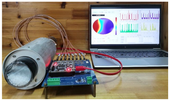
Figure 6.
ECT experimental setup with the room-temperature working medium.
Four particulate materials with the relative dielectric permittivity ratio with air close to the LN2-VN2 pair are chosen as the working fluids, as listed in Table 3. The eight-electrode sensor here is a quartz glass tube with an outer diameter of 60 mm and a thickness of 2 mm. Each electrode attached to the pipe has a length of 90 mm and a circumferential coverage rate of 80%.
Table 3.
The relative permittivity of materials for the alterative experiment at 300 K.
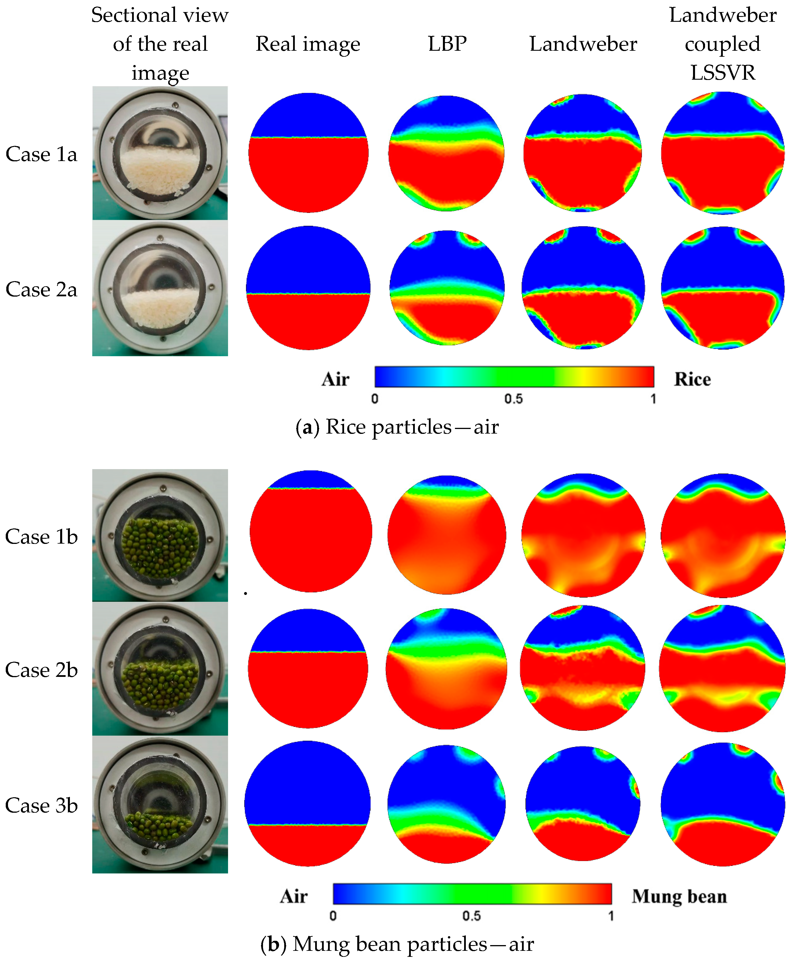
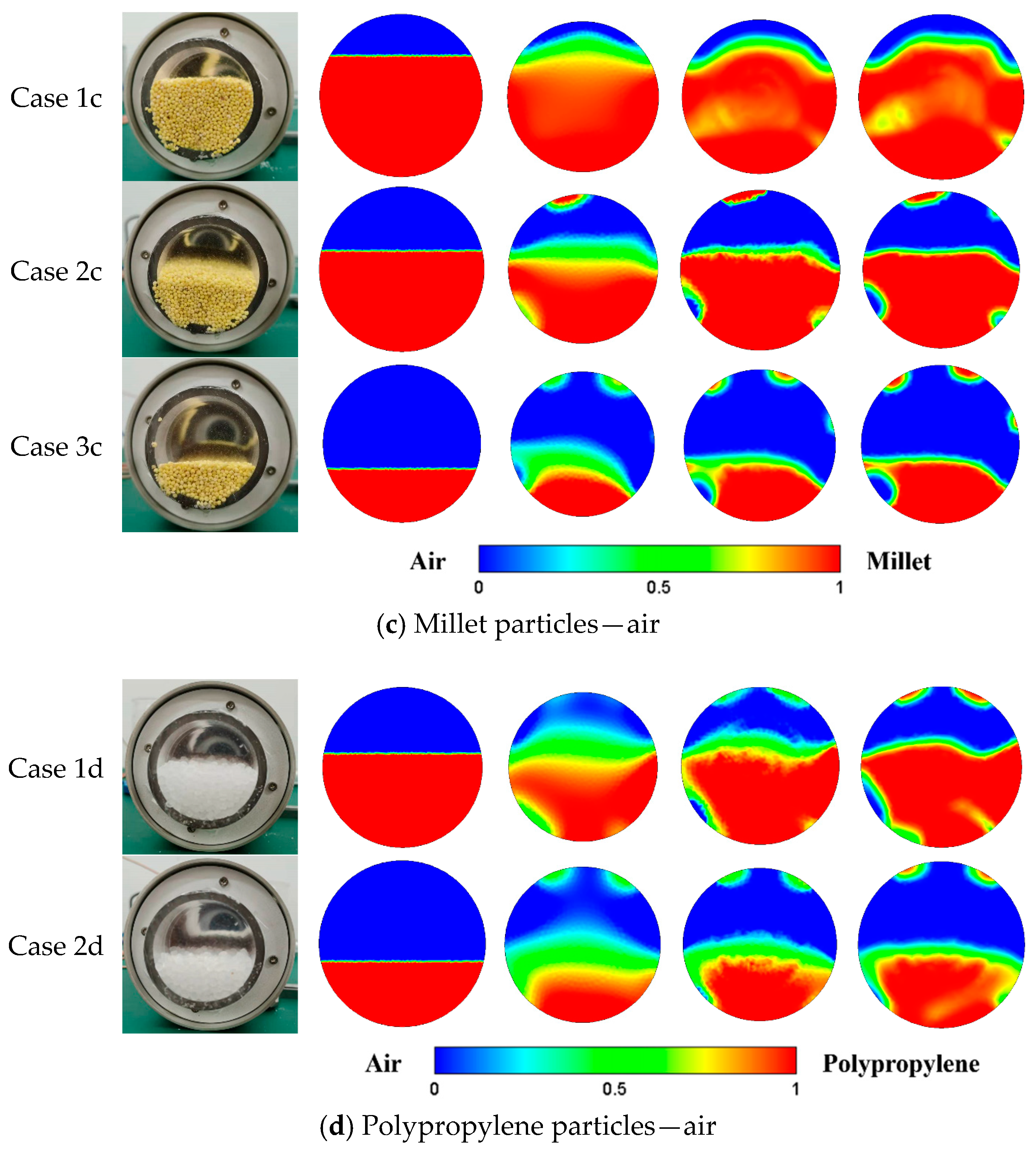
The stratified distributions with different holdups are reconstructed by the ECT with the LBP algorithm, the Landweber algorithm, and the Landweber coupled LSSVR algorithm. The real and inversed images of the polypropylene, mung bean, millet, and rice particles are shown in Figure 7, where the red part represents the alternative particles and the remaining blue part represents the air. The left column is the sectional view of the real distribution, and the second column is the real distribution mapped to the computational domain according to the real distribution for further data analysis. The other three columns are the inversed distributions based on the LBP, Landweber, and Landweber coupled LSSVR algorithm, respectively.

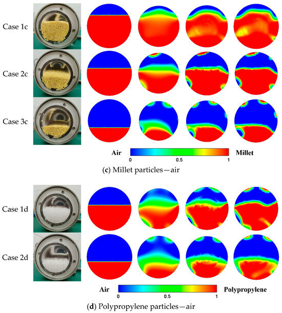
Figure 7.
Distributions and reconstruction images by ECT of (a) rice particles—air, (b) mung bean particles—air, (c) millet particles—air, and (d) polypropylene particles—air.
The void fraction (VF), the image error (IE), and the correlation coefficient (CC) are used to quantitatively evaluate the algorithms, which reflect the difference between the reconstruction results and the real images [26], and the calculated results are shown in Table 4, Table 5 and Table 6.
Table 4.
VF errors of three algorithms in the alternative experiment.
Table 5.
CCs of three algorithms in alternative experiment.
Table 6.
IEs of three algorithms in the alternative experiment.
is an normalized dielectric permittivity distribution vector of reconstruction results. is the normalized dielectric permittivity distribution vector of the real distribution. and are the average values of and , respectively. IE is the ratio of the modulus of the error vector between the inversion result and the real distribution represented by the vector and the modulus of the real distribution vector. It can not only represent the accuracy of the relative proportion of the inversion result but also the coincidence between the inversion result and the real distribution. The smaller the image error, the better the inversion result. CC represents the degree of coincidence between the inversion results and the relative positions of the real distribution. The closer the correlation coefficient is to 1, the higher the accuracy of the inversion results will be.
From the imaging results of the tentative experiments, the particle–air interfaces can be distinguished in most cases. The Landweber coupled LSSVR algorithm can reduce the error of Landweber algorithms in most cases, especially in Case 1b, where the LSSVR method improves the CC by 9.95% and decreases the IE and VF error by 14.619% and 2.336%, respectively. All the CCs of the Landweber coupled LSSVR algorithm exceed 0.82. At the same time, the interface is clearer, with fewer artifacts compared to those of the LBP and Landweber algorithms. The Landweber coupled LSSVR algorithm reaches the lowest IE of 34.736, which reduces 23.257% of the IE compared with the Landweber algorithm, and the highest CC of 0.895 in Case 2d. The tentative experiment results show that the three ECT algorithms are convenient to inverse the distribution of the fluid with relatively small dielectric relative permittivity, compared with the water/air flow (77.747/1.0005), and the LSSVR method can diminish the error of the Landweber algorithm to a certain extent.
4.2. Cryogenic Experiments
In the cryogenic experiments, there is no frosting outside the experimental pipe, due to the protection of the nitrogen vaporous in the chamber, while the outside surface of the chamber will cause frosting for a long time, which does not affect the sight after the frost is manually cleaned. The evaporation of LN2 inside the pipe is not intense and the LN2 level can be kept stable and observed without intensive boiling; therefore, the reconstruction images can reflect the real distribution of cryogenic flow.
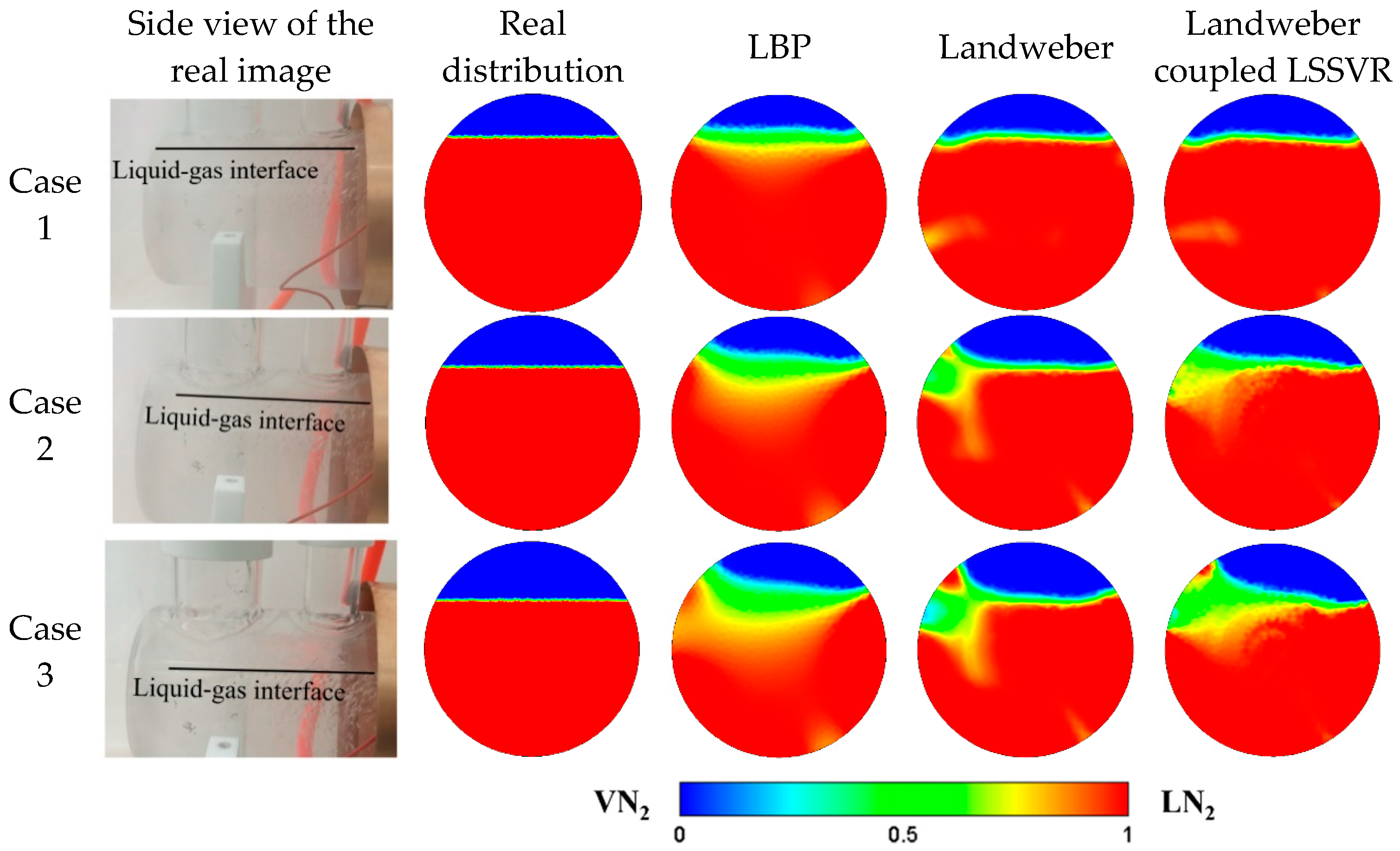
The image reconstruction results of the LN2-VN2 two-phase flow based on the ECT experimental facility are shown in Figure 8, where the red part represents the liquid phase and the remaining part represents the gas phase. The left column shows the real images of the experimental pipe with LN2 inside. An extra black line is added to the figure to clarify the position of the liquid level. The second column shows the real distribution mapped to the computational domain according to the liquid level measurement. The other columns in the figure provide the image reconstruction results based on the LBP, Landweber, and Landweber coupled LSSVR algorithm, respectively.
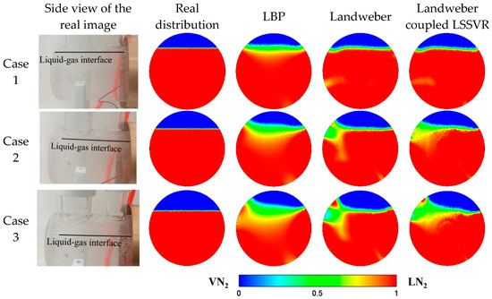
Figure 8.
Real LN2-VN2 distributions and reconstruction images by ECT.
The LSSVR hyperplane is trained by 4000 2D simulation samples the parameter selections of which are listed in Table 2. In the simulation sample generation processes, the relative dielectric permittivities of the high-permittivity phase and the low-permittivity phase are set to 1.4 and 1.0, respectively, and the relative dielectric permittivity of the pipe wall is set to 3.8.
By comparing the reconstruction images with the real phase distribution, the phase interface, which indeed reflects the real LN2 level in the pipe, can be captured in all the reconstructed images. The results indicate that the ECT system can image the cryogenic capacitance data with considerable accuracy, and the three reconstruction algorithms all can reconstruct the phase distribution.
In the reconstruction images, the artifact appears at the position of the No.1 electrode (see Figure 3) in Case 2 and Case 3. The artifact refers to the liquid-phase inclusion at the edge of the measurement area where no liquid phase exists in the real phase distribution. For the artifact, another kind of error, known as distortion, appears at the phase interface, blurring the boundary of the two phases and distorting the shape of the boundary line. Compared with the other two algorithms, the distortion of the projected LBP algorithm at the gas–liquid interface is the largest. The real interface can be approximately inferred from the image and the results of the projected LBP algorithm.
The projected Landweber iteration algorithm, the result of which shows the largest artifact at the wall of the measurement area in the cases mentioned above, achieves a more accurate result at the phase boundary in Case 1. However, while the distortions at the phase interface are partly reduced, the boundary line is distorted, especially in Case 3, causing the disturbance while clarifying the flow form, compared with the projected LBP algorithm.
Based on the results of the general Landweber algorithm, the Landweber coupled LSSVR algorithm strengthens the advantage of Landweber and decreases the distortion effect at the phase boundary. In terms of quantitative parameters, the results of CCs, IEs, and VF errors for the three algorithms are presented in Table 7. The Landweber coupled LSSVR algorithms obtain the best performance among these three algorithms with all the CCs beyond 0.88, especially in Case 1, where the artifacts of reconstructions are shown to be the smallest, the error of the void fraction of the Landweber coupled LSSVR algorithm fits the real distribution with a VF difference of 1.201%, while the VF error reaches 6.212% of the LBP algorithm and 4.508% of general Landweber algorithm. The CC of the modified algorithm reaches the highest of 0.975 in this case. As the artifacts appear in Case 2 and Case 3, the goodness of fit by LBP and Landweber becomes poorer in either VF, CC, or IE. Although the LSSVR method cannot eliminate the impact of artifacts, it makes up for the lack of imaging quality of the Landweber algorithm by clearing the boundary of different phases, and it has achieved good results in quantitative data. In Case 2, the VF error decreased by 5.777% compared with the Landweber algorithm and 11.082% with the LBP algorithm. This phenomenon can be observed in the result of the tentative experiment in Case 3c, where the CC increased from 0.772 to 0.827. Additionally, the LSSVR method can improve the void fraction measurement by optimizing the influence of the distortion of the phase interface which is shown in the results of Case 1c. The phase interface is severely distorted into a curve in this case, while the LSSVR method successfully reduces the VF error so that the void fraction information is more accurate at the expense of the reduction of the CC and image quality.
Table 7.
VF errors, CCs, and IEs of cryogenic experiment cases for different algorithms.
The causes of the distortion at the edge of the gas–liquid phase are the nonlinear error of the algorithm and the slight evaporation of the LN2, which only fuzzes the boundary between the gas and liquid phases and is not capable of changing the geometric shape of the dividing line.
Based on these preliminary experiments, it is reasonable to believe that the Landweber coupled LSSVR can be applied to the detection of other cryogenic working fluids with higher saturation temperatures, such as liquid oxygen and liquefied natural gas (LNG), with improved performance compared with the counterpart.
5. Conclusions
In this paper, electronic capacitance tomography was applied to measure the phase distribution of four alternative working fluids at room temperature and LN2-VN2 flow. The alternative experiment showed the potential of applying the projected LBP algorithm, the projected Landweber iteration algorithm, and the projected Landweber iteration coupled LSSVR algorithm to the inversion imaging of the two-phase flow with a relative dielectric permittivity ratio close to 1.6. In the cryogenic experiment, the interface of the different LN2 levels of the stratified flow was detected and imaged. The Landweber coupled LSSVR algorithm presented the best performance on image reconstruction, which reached the smallest VF error of 0.554% and highest CC of 0.975. While the projected LBP algorithm achieved a relatively fuzzy image and acceptable image reconstruction quality, the Landweber iteration algorithm reached the highest accuracy in VF, with an error of 4.509%, although it produced distortion at the interface and the edge of the computational domain. The LSSVR method can improve the performance of the Landweber algorithm. Strengthening the advantage of the Landweber algorithm, the modified algorithm presents a clearer phase interphase. However, it cannot eliminate the artifacts at the boundary of the computational region—considering that it inherited from the Landweber algorithm the artifacts brought by the Landweber algorithm, such artifacts are inevitable. The reason is that the LSSVR coupled algorithm is a fusion-driven method—its modification is based on the error capacitance. The error capacitance is obtained from the calculation result from the linear algorithm, and the reconstructed distribution vector’s dimensionality is reduced by the sensitivity matrix. This downsampling process has lost some information; thus, as an additional correction, the modification results will not deviate too far from the original algorithm. However, the error capacitance term is optimized by LSSVR based on the trained samples, and the improvement can be observed, which is reflected by the quality evaluation from CCs, IEs, and VF errors.
The reconstruction experiment verified that the Landweber coupled LSSVR algorithm is a promising algorithm employed for ECT phase distribution detection for cryogenic two-phase flow.
Author Contributions
Conceptualization, Z.-N.T. and T.X.; methodology, Z.-N.T. and T.X.; software, Z.-N.T.; validation, Z.-N.T., X.-X.G. and T.X.; formal analysis, Z.-N.T.; investigation, T.X.; resources, X.-B.Z.; data curation, Z.-N.T.; writing—original draft preparation, Z.-N.T. and X.-B.Z.; writing—review and editing, Z.-N.T. and X.-B.Z.; visualization, Z.-N.T.; supervision, X.-B.Z.; project administration, X.-B.Z.; funding acquisition, X.-B.Z. All authors have read and agreed to the published version of the manuscript.
Funding
This work was supported by the Nature and Science Foundation of China (No. 51976177) and the National Key Research and Development Program of China (No. 2021YFB4000700).
Data Availability Statement
The data presented in this study are available on request from the corresponding author. The data are not publicly available due to commercial privacy.
Conflicts of Interest
The authors declare no conflict of interest.
Nomenclature
| a | Linear offset vector of LSSVR | Normalized sensitive field matrix | |
| b | Coefficient vector of LSSVR | Normalized sensitive field between the measuring electrode i and j | |
| C | Capacitance value | Excitation voltage | |
| Normalized vector of dielectric permittivity distribution | Residual error of normalized capacitance | ||
| Kernal function | Greek symbol | ||
| M | Total number of effective capacitance values | ||
| N | Total number of grid cells | Iteration step size | |
| Unit normal vector at the wall | Electrode position | ||
| Electric potential distribution | Dielectric permittivity distribution | ||
| P(.) | Projection operation | Normalized measured capacitance vector | |
| Q | Quantity of electric charge | Computational domain | |
| Sensitive field between the measuring electrode i and j | Boundary of the computational domain which is not covered by the electrode area | ||
References
- Sakamoto, Y.; Kobayashi, H.; Naruo, Y.; Takesaki, Y.; Nakajima, Y.; Furuichi, A.; Tsujimura, H.; Kabayama, K.; Sato, T. Investigation of the Void Fraction–quality Correlations for Two-phase Hydrogen Flow Based on the Capacitive Void Fraction Measurement. Int. J. Hydrogen Energy 2019, 44, 18483–18495. [Google Scholar] [CrossRef]
- Yang, Z.Q.; Chen, G.F.; Zhuang, X.R.; Song, Q.L.; Deng, Z.; Shen, J.; Gong, M.Q. A New Flow Pattern Map for Flow Boiling of R1234ze(E) in a Horizontal Tube. Int. J. Multiph. Flow 2018, 98, 24–35. [Google Scholar] [CrossRef]
- Forte, G.; Clark, P.; Yan, Z.; Stitt, E.H.; Marigo, M. Using a Freeman Ft4 Rheometer and Electrical Capacitance Tomography to Assess Powder Blending. Powder Technol. 2018, 337, 25–35. [Google Scholar] [CrossRef]
- Chen, J.Y.; Wang, Y.C.; Zhang, W.; Qiu, L.M.; Zhang, X.B. Capacitance-based Liquid Holdup Measurement of Cryogenic Two-phase Flow in a Nearly-horizontal Tube. Cryogenics 2017, 84, 69–75. [Google Scholar] [CrossRef]
- Khalil, A.; Mcintosh, G.; Boom, R. Experimental Measurement of Void Fraction in Cryogenic Two Phase Upward Flow. Cryogenics 1981, 21, 411–414. [Google Scholar] [CrossRef]
- Filippov, Y.P.; Kovrizhnykh, A.M.; Miklayev, V.M.; Sukhanova, A.K. Metrological Systems for Monitoring Two-phase Cryogenic Flows. Cryogenics 2000, 40, 279–285. [Google Scholar] [CrossRef]
- Filippov, Y.P. How to Measure Void Fraction of Two-phase Cryogenic Flows. Cryogenics 2001, 41, 327–334. [Google Scholar] [CrossRef]
- Filippov, Y.P.; Kakorin, I.; Kovrizhnykh, A.M. New Solutions to Produce a Cryogenic Void Fraction Sensor of Round Cross-section and Its Applications. Cryogenics 2013, 57, 55–62. [Google Scholar] [CrossRef]
- Harada, K.; Murakami, M.; Ishii, T. PIV Measurements for Flow Pattern Void Fraction in Cavitating Flows of He II and He I. Cryogenics 2006, 46, 648–657. [Google Scholar] [CrossRef]
- Che, H.Q.; Ye, J.M.; Tu, Q.Y.; Yang, W.Q.; Wang, H.G. Investigation of Coating Process in Wurster Fluidised Bed Using Electrical Capacitance Tomography. Chem. Eng. Res. Des. 2018, 132, 1180–1192. [Google Scholar] [CrossRef]
- Guo, Q.; Ye, M.; Yang, W.Q.; Liu, Z. A Machine Learning Approach for Electrical Capacitance Tomography Measurement of Gas–solid Fluidized Beds. Aiche J. 2019, 65, e16583. [Google Scholar] [CrossRef]
- Mohamad, E.J.; Rahim, R.A.; Rahiman, M.H.F.; Ameran, H.L.M.; Muji, S.Z.M.; Marwah, O.M.F. Measurement and Analysis of Water/oil Multiphase Flow Using Electrical Capacitance Tomography Sensor. Flow Meas. Instrum. 2016, 47, 62–70. [Google Scholar] [CrossRef]
- Yang, W.Q.; Stott, A.L.; Beck, M.S.; Xie, C.G. Development of Capacitance Tomographic Imaging Systems for Oil Pipeline Measurements. Rev. Sci. Instrum. 1995, 66, 4326–4332. [Google Scholar] [CrossRef]
- Ortiz-alemán, C.; Martin, R. Inversion of Electrical Capacitance Tomography Data By Simulated Annealing: Application to Real Two-phase Gas–oil Flow Imaging. Flow Meas. Instrum. 2005, 16, 157–162. [Google Scholar] [CrossRef]
- Ismail, I.; Gamio, J.; Bukhari, S.; Yang, W.Q. Tomography for Multi-phase Flow Measurement in the Oil Industry. Flow Meas. Instrum. 2005, 16, 145–155. [Google Scholar] [CrossRef]
- Dyakowski, T.; Edwards, R.B.; Xie, C.G.; Williams, R.A. Application of Capacitance Tomography to Gas-solid Flows. Chem. Eng. Sci. 1997, 52, 2099–2110. [Google Scholar] [CrossRef]
- Cui, Z.Q.; Yang, C.Y.; Sun, B.Y.; Wang, H.X. Liquid Film Thickness Estimation Using Electrical Capacitance Tomography. Meas. Sci. Rev. 2014, 14, 8–15. [Google Scholar] [CrossRef]
- Román, A.; Cronin, J.; Ervin, J.; Byrd, L. Measurement of the Void Fraction and Maximum Dry Angle Using Electrical Capacitance Tomography Applied to a 7 mm Tube with R-134a. Int. J. Refrig. 2018, 95, 122–132. [Google Scholar] [CrossRef]
- Xie, H.J.; Chen, H.; Gao, X.; Zheng, X.D.; Zhi, X.Q.; Zhang, X.B. Theoretical Analysis of Fuzzy Least Squares Support Vector Regression Method for Void Fraction Measurement of Two-phase Flow by Multi-electrode Capacitance Sensor. Cryogenics 2019, 103, 102969. [Google Scholar] [CrossRef]
- Xie, H.J.; Xia, T.; Tian, Z.N.; Zheng, X.D.; Zhang, X.B. A Least Squares Support Vector Regression Coupled Linear Reconstruction Algorithm for ECT. Flow Meas. Instrum. 2021, 77, 101874. [Google Scholar] [CrossRef]
- Xia, T.; Xie, H.J.; Wei, A.B.; Zhou, R.; Qiu, L.M.; Zhang, X.B. Preliminary Study on Three-dimensional Imaging of Cryogenic Two-phase Flow Based on Electrical Capacitance Volume Tomography. Cryogenics 2020, 110, 103127. [Google Scholar] [CrossRef]
- Hunt, A.; Rusli, I.; Schakel, M.; Kenbar, A. High-speed Density Measurement for Lng and Other Cryogenic Fluids Using Electrical Capacitance Tomography. Cryogenics 2021, 113, 103207. [Google Scholar] [CrossRef]
- Sun, S.J.; Zhang, W.B.; Sun, J.T.; Cao, Z.; Xu, L.J.; Yan, Y. Real-Time Imaging and Holdup Measurement of Carbon Dioxide Under CCS Conditions Using Electrical Capacitance Tomography. IEEE Sens. J. 2018, 18, 7551–7559. [Google Scholar] [CrossRef]
- Tian, Z.; Gao, X.; Qiu, L.; Zhang, X. Experimental imaging and algorithm optimization based on deep neural network for electrical capacitance tomography for LN2-VN2 flow. Cryogenics 2022, 127, 103568. [Google Scholar] [CrossRef]
- Gao, X.; Tian, Z.; Qiu, L.; Zhang, X. A hybrid deep learning model for ECT image reconstruction of cryogenic fluids. Flow Meas. Instrum. 2022, 87, 102228. [Google Scholar]
- Xie, C.G.; Huang, S.M.; Hoyle, B.S.; Thorn, R.; Lenn, C.; Snowden, D.; Beck, M.S. Electrical capacitance tomography for flow imaging system model for development of image reconstruction algorithms and design of primary sensors. Proc. G Circuits Devices Syst. 1992, 139, 89–98. [Google Scholar] [CrossRef]
- Yang, W.Q.; Spink, D.M.; York, T.A.; McCann, H. An Image-reconstruction Algorithm Based on Landweber’s Iteration Method for Electrical-capacitance Tomography. Meas. Sci. Technol. 1999, 10, 1065–1069. [Google Scholar] [CrossRef]
- Soleimani, M.; Lionheart, W.R.B. Nonlinear Image Reconstruction for Electrical Capacitance Tomography Using Experimental Data. Meas. Sci. Technol. 2005, 16, 1987–1996. [Google Scholar] [CrossRef]
- Liu, S.; Fu, L.; Yang, W.Q. Optimization of an Iterative Image Reconstruction Algorithm for Electrical Capacitance Tomography. Meas. Technol. 1999, 10, 1970–1980. [Google Scholar] [CrossRef]
- Wang, H.X.; Tang, L.; Cao, Z. An Image Reconstruction Algorithm Based on Total Variation with Adaptive Mesh Refinement for ECT. Flow Meas. Instrum. 2007, 18, 262–267. [Google Scholar] [CrossRef]
- Li, Y.; Yang, W.Q. Image Reconstruction by Nonlinear Landweber Iteration for Complicated Distributions. Meas. Sci. Technol. 2008, 19, 94014. [Google Scholar] [CrossRef]
- Yang, W.Q.; Liu, S. Electrical Capacitance Tomography with Square Sensor. Electron. Lett. 1999, 35, 295–296. [Google Scholar] [CrossRef]
- Xie, H.J.; Yu, L.; Zhou, R.; Qiu, L.M.; Zhang, X.B. Preliminary Evaluation of Cryogenic Two-phase Flow Imaging Using Electrical Capacitance Tomography. Cryogenics 2017, 86, 97–105. [Google Scholar] [CrossRef]
- Cui, Z.Q.; Wang, Q.; Xue, Q.; Fan, W.R.; Zhang, L.L.; Cao, Z.; Sun, B.Y.; Wang, H.X.; Yang, W.Q. A Review on Image Reconstruction Algorithms for Electrical Capacitance/resistance Tomography. Sens. Rev. 2016, 36, 429–445. [Google Scholar] [CrossRef]
- Isaksen, Ø. A Review of Reconstruction Techniques for Capacitance Tomography. Meas. Sci. Technol. 1996, 7, 325–337. [Google Scholar] [CrossRef]
- Liao, A.M.; Zhou, Q.Y. Application of ECT and Relative Change Ratio of Capacitances in Probing Anomalous Objects in Water. Flow Meas. Instrum. 2015, 45, 7–17. [Google Scholar] [CrossRef]
- Yang, W.Q.; Peng, L.H. Image Reconstruction Algorithms for Electrical Capacitance Tomography. Meas. Sci. Technol. 2003, 14, R1–R13. [Google Scholar] [CrossRef]
- Peng, L.H.; Merkus, H.; Scarlett, B. Using Regularization Methods for Image Reconstruction of Electrical Capacitance Tomography. Part. Part. Syst. Charact. 2000, 17, 96–104. [Google Scholar] [CrossRef]
- Yang, Y.J.; Peng, L.H. Data Pattern with ECT Sensor and Its Impact on Image Reconstruction. IEEE Sens. J. 2013, 13, 1582–1593. [Google Scholar] [CrossRef]
- Smits, G.F.; Jordaan, E.M. Improved SVM regression using mixtures of kernels. In Proceedings of the International Joint Conference on Neural Networks, IEEE Xplore, Honolulu, HI, USA, 12–17 May 2002; pp. 2785–2790. [Google Scholar]


Disclaimer/Publisher’s Note: The statements, opinions and data contained in all publications are solely those of the individual author(s) and contributor(s) and not of MDPI and/or the editor(s). MDPI and/or the editor(s) disclaim responsibility for any injury to people or property resulting from any ideas, methods, instructions or products referred to in the content. |
© 2023 by the authors. Licensee MDPI, Basel, Switzerland. This article is an open access article distributed under the terms and conditions of the Creative Commons Attribution (CC BY) license (https://creativecommons.org/licenses/by/4.0/).