Abstract
Abundant geothermal energy can be harvested from deep, low-permeability rocks using an enhanced geothermal system (EGS) that relies on an artificially created permeable fracture network through cold water injection. In this study, a two-way coupling technique for thermo-hydromechanical modeling was used to simulate hydraulic fracture propagation in an EGS. The transient heat and fluid flow in porous media were modeled using the finite volume method, while hydraulic fracture propagation and interaction with natural fractures were modeled using the variational phase-field method. Our findings underscore the importance of poroelastic and thermoelastic effects on fracture propagation in naturally fractured reservoirs. The results of this study demonstrate that thermo-hydromechanical processes are crucial elements in simulating and optimizing an enhanced geothermal reservoir system.
1. Introduction
Geothermal energy is the thermal energy generated and stored within the underground formations of the Earth. It is more environmentally friendly than conventional fuel sources because the carbon footprint of a geothermal power plant is low. Unlike wind and solar power, geothermal energy is as reliable as it is weather-independent. The International Renewable Energy Agency (IRENA) estimates that geothermal resources in formations less than 10 km deep contain 50,000 times more energy than all oil and gas resources worldwide [1]. As such, geothermal energy has received considerable attention as an alternative energy source, and the target consumption of geothermal sources should increase by 50% by 2050 [2].
Geothermal energy has been used for many years, but the first geothermal power generator was tested in Larderello, Italy, in 1904 [3]. Conventional geothermal systems usually target high-temperature permeable reservoirs where producing water can easily transport heat to the surface [4]. Although geothermal energy has vast potential in the deepest part of the Earth’s crust, there is an obstacle to extracting heat owing to the nature of extremely low permeability and/or a limited number of water resources.
In an enhanced geothermal system (EGS), water is actively injected to economically produce thermal energy from deep formations [5]. Water is injected under high pressure to initiate and extend fractures that enable that water to freely flow in and out of low-permeability formations. The first EGS operation, then called hot dry rock, was introduced by the Los Alamos National Laboratory in the United States in 1970 [6]. Since then, the EGS has received significant attention from researchers, highlighting its potential to not only contribute to sustainable energy production but also facilitate long-term energy security [7]. While hydraulic fracturing is widely used to enhance oil and gas production by enhancing their permeability, it is also applied to EGS because fracture distribution and bulk permeability are critical for commercial geothermal energy production [8].
Significant developments in hydraulic fracturing simulation have been achieved by utilizing a variety of methodologies to achieve greater accuracy. Most hydraulic fracturing models are based on linear elastic fracture mechanics (LEFM), as discussed by Adachi et al. [9]. Various discretization methods, such as the extended/general finite element method (XFEM) and the boundary element method (BEM) have been used to simulate hydraulic fracture growth. Yi et al. (2017) and Zarrinzadeh et al. (2020) [10,11] proposed XFEM for numerical methods; however, their models have limitations in resolving plane discontinuities with a fixed shape function, managing interactions between hydraulic and natural fractures, and being numerically unstable at times. McClure et al. (2015) [12] proposed a model for hydraulic fracture interacting with natural fractures using numerical BEM. They treated the primary fracture propagation in pseudo-3D and the interactions with natural fractures using semi-analytical crossing criteria (Gu and Weng, 2000) [13].
A promising alternative approach, known as the phase-field model of fractures, was conceived by Bourdin et al. (2000) [14] as a regularization technique of the variational approach to fractures [15]. Because of its ability to model complex fractures and handle fracture nucleation, this method has been extended to ductile [16], fatigue [17], and dynamic fractures [18,19]. Its application to hydraulic fractures was first proposed by Bourdin et al. (2012) [18] and extended to poroelastic media by Wheeler et al. (2014), Wilson and Landis (2016), Heider and Markert (2016), Chukwudozie et al. (2019), and Zhou et al. (2019) [20,21,22,23,24]. Another way to simulate fracture propagation within reservoirs is to couple a phase-field model with an external reservoir simulator [20,25]. This brings practical benefits because one can take full advantage of established reservoir simulators that may already be used for field development.
The economic success of an EGS depends on its sustainable thermal energy generation for an extended period [26]. EGS performance has been studied using thermo-hydraulic-mechanical (THM) numerical simulators [27,28,29,30,31,32,33]. Ref. [27] presented a fully coupled THM model to evaluate the effects of fracture spacing, well inclination, and water mass flow rates on energy production rates during the life span of an EGS. Their model assumed static fracture geometries and ignored the geomechanical effects. Ref. [28] developed a fully coupled fluid flow–geomechanical model using TOUGH2-EGS to analyze pressure and temperature changes and rock deformation treatments in stress-sensitive permeability based on a relationship between mean normal stress and volumetric strain. Ref. [29] developed a multi-fracture system and evaluated its heat extraction performance by considering the actual fracture width of newly formed fractures using the simulation FLAC3-TOUGH2MP-TMVOC. Ref. [30] proposed pumping cold water through an injection well connected to a production well via a single fracture. During cold water injection, either a fracture or a crack is created along with a well connection, and a coupled THM simulation is then performed to estimate the fracture opening because of rapid temperature decline and reduced energy production. Refs. [31,32] have employed Tough-Frac and Tough2Biot simulators to conduct comprehensive thermal, hydraulic, and mechanical (THM) modeling of hydro shearing stimulation. These simulations specifically focused on volcanic rock formations that contains low conductivity fractures and on an Enhanced Geothermal System (EGS).
In previous coupling simulation studies, there have been limitations. Ref. [28] presented a fully coupled model using TOUGH2-EGS. However, they simplified the geomechanics equation and did not consider a full stress tensor in their model. Another simulation [27] also presented a hydrothermal model evaluating heat production in an EGS. However, their model ignored geomechanical effects, which are a crucial element in the EGS process. Refs. [29,30] presented a THM model analyzing the mechanical deformation of reservoir rock experienced during the EGS process. However, dynamic fracture growth was not considered in their work. This study uses the phase-field method to overcome the limitations of the previous studies. The phase-field method can define fracture propagation in an EGS site to account for existing natural fractures. Furthermore, it can handle heterogeneous properties and consider geomechanical effects that previous studies did not. Refs. [31,32,33] utilized a coupled reservoir simulator and mechanical model; however, it did not incorporate changes in the viscosity and water density resulting from temperature changes.
Another prior study [20] investigated hydromechanical coupling using a phase-field model to treat slick water hydraulic fracturing. Ref. [20] added a penalization term to the functional energy equation by including fracture growth to calculate the energy release rate associated with fracture growth. The growth direction of this fracture follows the entropy change process spontaneously according to the second law of thermodynamics. Another coupling simulation, THM, by Lie et al. (2023) [34], however, does not consider the thermal effect on stress and changes in fluid properties at high temperatures. However, the simulation in this prior research did not consider the influence of temperature change. In our paper, we investigated the effect of temperature on the phase-field method in predicting fracture propagation.
The permeability of the fractured rock is modeled as a function of the phase-field variable increasing as the fracture grows. Numerous studies have explored the influence of heat on fracture propagation using various methods, including the phase-field approach. In this study, our primary focus is on the alternative algorithm developed for fracture prediction analysis. We propose an iteratively coupled thermo-hydromechanical model for hydraulic fracturing to evaluate the importance of poroelastic and thermoelastic effects on fracture growth experienced by an enhanced geothermal system (EGS). This model can be coupled using external heat flow simulation. The thermal flow element of our model was based on the general-purpose finite volume method, code MRST-AD, developed by [35]. The geomechanical calculation was based on the variational phase-field model of hydraulic fractures [36] with thermoelastic effects, which were also implemented in this study.
2. Mathematical Model
In EGS stimulation, cold water was injected into a rock formation, inducing significant temperature and pressure changes around the wellbore. In this study, the mass and energy balance equations were solved for mass and heat flow in the reservoir and fractures. In addition, the fracture propagation was modeled using a phase-field approach, taking into account poroelasticity and thermoelasticity. The following sections describe the governing equations of the EGS simulator developed in this study.
2.1. Mechanical Equilibrium and Phase-Field Equations
Consider a domain, Ω, in , where N = 2 and N = 3 for 2 and 3D. The domain contains a brittle elastic material with a stiffness tensor, C. The body force component represents b(x,t) per unit mass, as defined in Ω. The external forces are denoted by τ(x,t) and applied to with the normal vector (Figure 1). The boundary condition for displacement is denoted by g(x,t) and is defined as The domain has a fracture set, , and denotes the fracture normal vector.
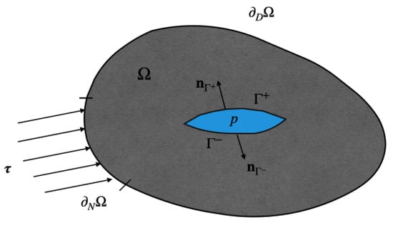
Figure 1.
Determination of fractures in porous media by calculating elements of the unstructured domain elements.
The static equilibrium is provided by
where is the stress tensor. The boundary conditions are expressed by
Because the fluid pressure inside the fracture acts as traction on the fracture surfaces, , the following boundary conditions are imposed on the fracture surface:
By considering the pressure exerted by fluids in a porous medium, the total stress imposed on the object can be expanded into
where is the bulk modulus of the material, is the effective stress, and is Biot’s coefficient. The constitutive relation of the poroelastic material is as follows:
The total strain field is further decomposed into thermal strain, , and elastic strain, , as
Elastic strain as the ratio of total strain to elastic strain is
The thermal strain for the isotropic rock mass is calculated from
Substituting Equation (10) into Equation (9) and noting that the elastic strain satisfies Equation (6) yields
According to Griffith’s criterion [37], the fracture extends when the energy release rate, , reaches the critical value as
For any kinematically admissible displacement, u, the total external work, , is calculated as the sum of the work performed by the body force and the external load as
The potential energy, , consists of the elastic energy of the system and the external work as follows:
In Equation (13), is the thermo-poroelastic strain energy density, which we define as
According to [15], who presented a variational approach to fractures, the total energy is the sum of the potential energy and surface energy required to produce a fracture set, :
where the fracture length in 2D is represented by the surface integral of the fracture set, . Substituting Equations (12) and (13) and adding the work performed by the fluid pressure on the crack faces provides the following:
The solution to Equation (16) involves discontinuously deforming the cracks, , which poses significant challenges in terms of numerical implementation. For numerical implementation, refs. [14,38] introduced the regularization parameter ls, defining the fracture with a smooth phase-field function, v, which varies between 0 and 1. The phase-field variable,, represents the status of the material in a diffused manner, where denotes an intact material and represents a fully broken material. The transition length from the intact to the fully broken state of the material depends on the regularization length, . The total energy in Equation (16) can be approximated as follows [12]:
2.2. Mass Balance and Momentum Balance Equations
A single-phase water flow system was assumed in this study. The mass conservation for the fluid phase of the porous medium can be written as
where is the porosity, is the water density, is the Darcy flux vector, and q is the mass source or sink term. The variation in pore volume with pore pressure can be accounted for by the pressure dependence of the porosity. Assuming that the porosity is expressed by a linear function of pressure [39], the rock porosity at any pressure can be expressed as
where is the initial pressure at which the porosity is , and is the porosity compressibility.
The water density is assumed to change with temperature and pressure as
where and are the saturation density and compressibility of water, respectively, which may be obtained by [40]
Referring to Darcy’s law of single-phase liquid flow, the Darcy velocity, , is provided by
where is the intrinsic permeability tensor of a porous medium, is the water viscosity, is the gravitational constant, and is the elevation.
It is assumed that the water viscosity changes with temperature according to the following equation [41]:
2.3. Energy Balance Equation
Assuming that the rock and fluid are in local thermal equilibrium (that is, there is no heat moving between the solid and fluid phases), the energy balance equation can be represented by
where is the rock density, is the specific heat of the rock, is the temperature, is the average thermal conductivity, and is the energy source term. In addition, and are the specific internal energy and specific enthalpy of water, respectively, which can be calculated as follows [40]:
where is the saturation-specific internal energy, and is the specific heat of water. The values of and are obtained with curve fitting and approaching with IAPWS-If97 [42].
2.4. System of Equations and Coupling Technique
The primary variables of the thermo-hydromechanical model developed in this study were pressure (), temperature (), displacement (), and the phase-field variable (). The mass balance equation, energy balance equation, and phase-field equation must be solved using an adequate coupling technique.
The effect of fractures on fluid flow is determined by introducing a permeability multiplier, where the Darcy velocity (Equation (23)) can be expressed as
where is the scalar permeability multiplier, which can be computed as a function of the phase-field variable, v [25]:
where and are the permeability of the fracture and matrix, respectively, and is the threshold phase-field value wherein the permeability changes from a matrix to fracture permeability.
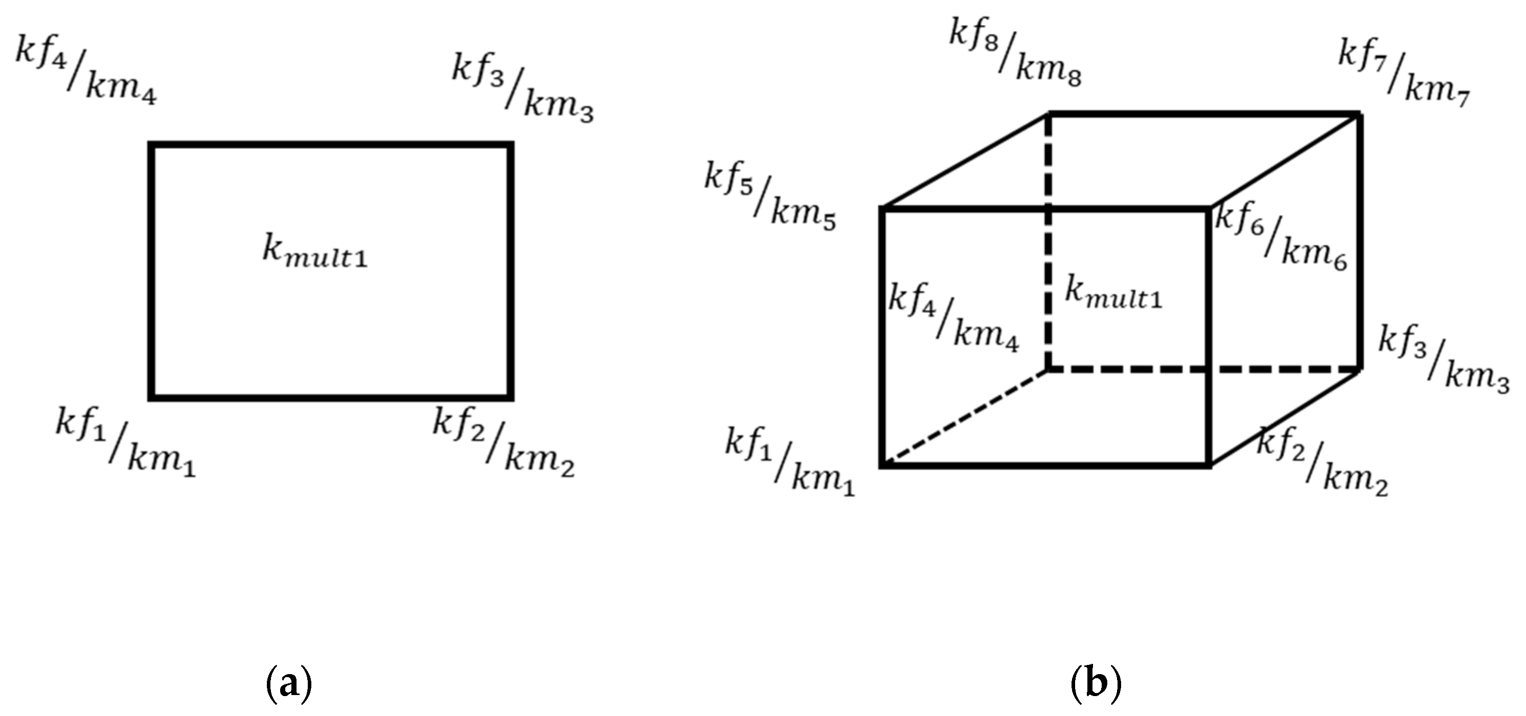
For numerical implementation, the open-source codes MATLAB Reservoir Simulation Toolbox (MRST) [35] and OpenGeosys [23] were coupled in this study. The thermo–hydro simulation was conducted using the MRST, and the permeability multipliers are updated at each nonlinear iteration between the two models. After each iteration, the pressure and temperature are sent to the phase-field fracture code implemented in OpenGeosys, and the permeability multipliers are received. Because the phase-field equation is discretized using the finite element method, the phase-field variables are computed at each node. For this study, an eight-node linear element was employed (Figure 2), and the permeability multiplier used for the flow code was computed using the following formula:

Figure 2.
Location of phase-field variables and permeability multiplier calculated for each element: (a) 2D element and (b) 3D element.
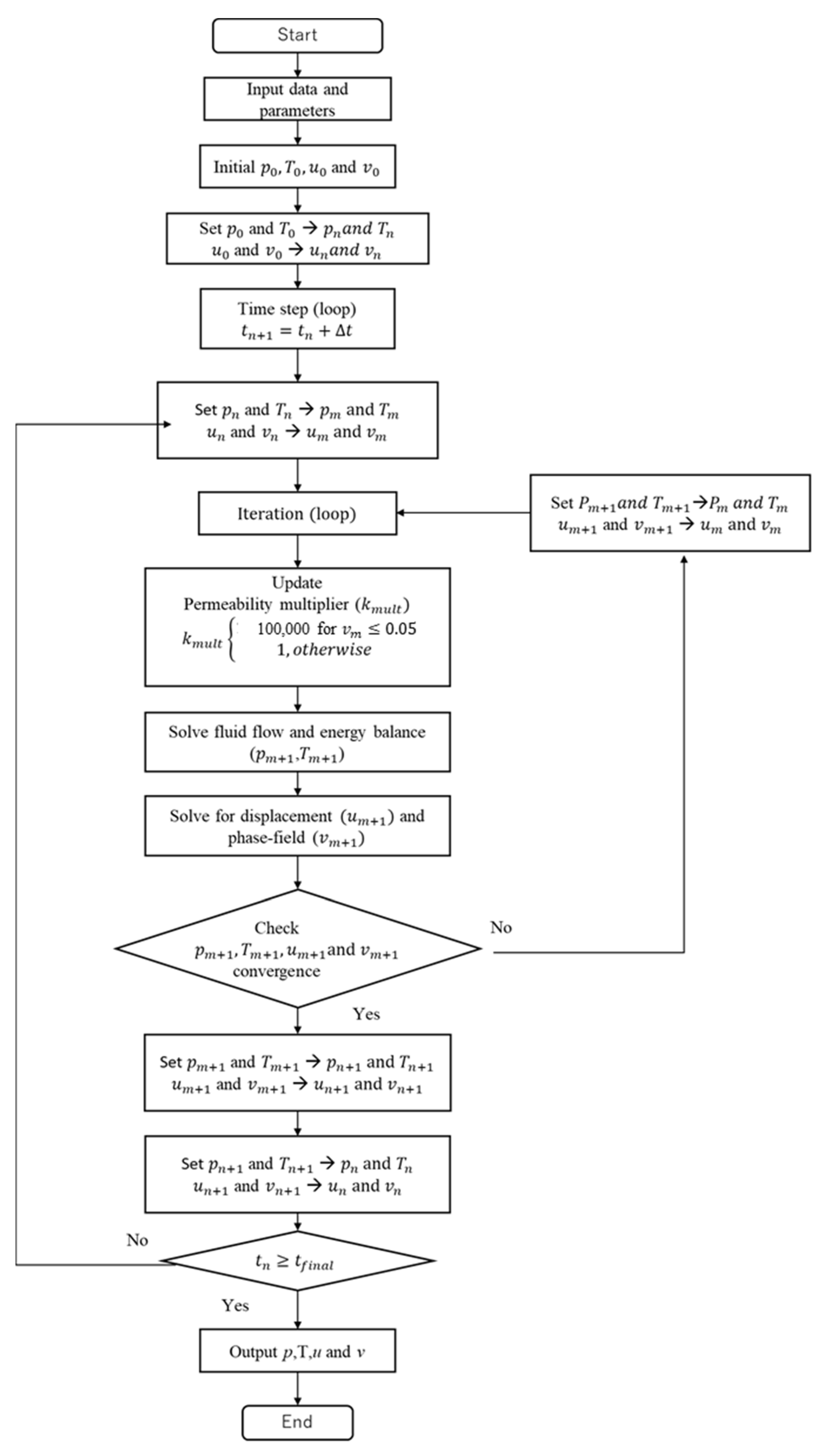
The algorithm used to solve for the four primary unknowns (, and ) is summarized in Figure 3.
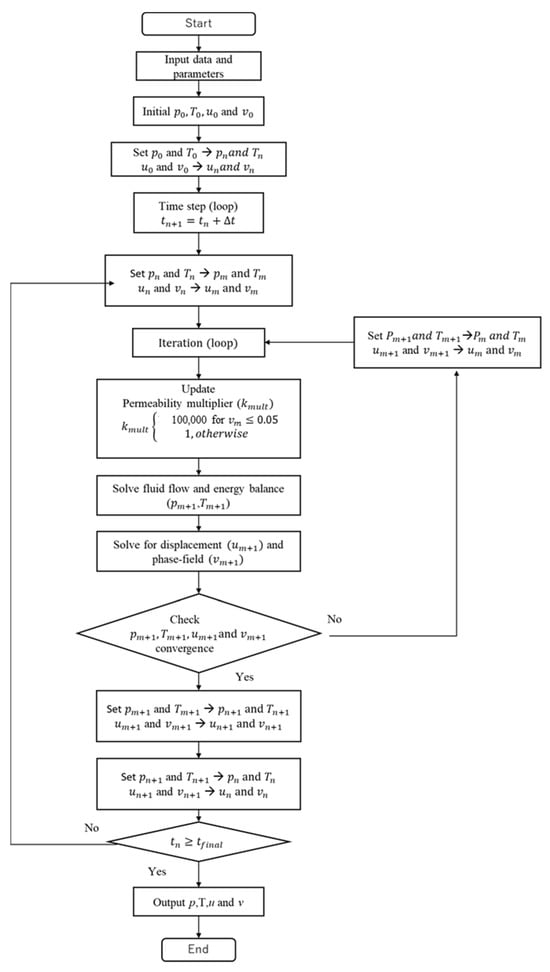
Figure 3.
Workflow of thermo-hydromechanical simulation for hydraulic fracturing analysis in an EGS.
2.5. Verification
In this section, the coupled MRST–phase-field model is verified by comparing its simulation results against the semi-analytical solution presented in [43], which addresses the deviation from the K-vertex by offering accurate approximations for the time evolution of the fracture opening displacement, fracture length, and fluid pressure as functions of .
The semi-analytical solution presented in reference [43] addresses the deviation from the K-vertex by offering accurate approximations for the time evolution of the fracture opening displacement, fracture length, and fluid pressure as functions of :
where . The computational domain is assumed a square region of 100 m × 100 m. The initial fracture with the length of 4 m, which is located at the center of the domain, is assumed. Fluid is injected into the center of the fracture at a constant rate. The rock and fluid properties, injection rate, and model parameters used in the simulation are summarized in Table 1.

Table 1.
The values for reservoir and fluid in this computation.
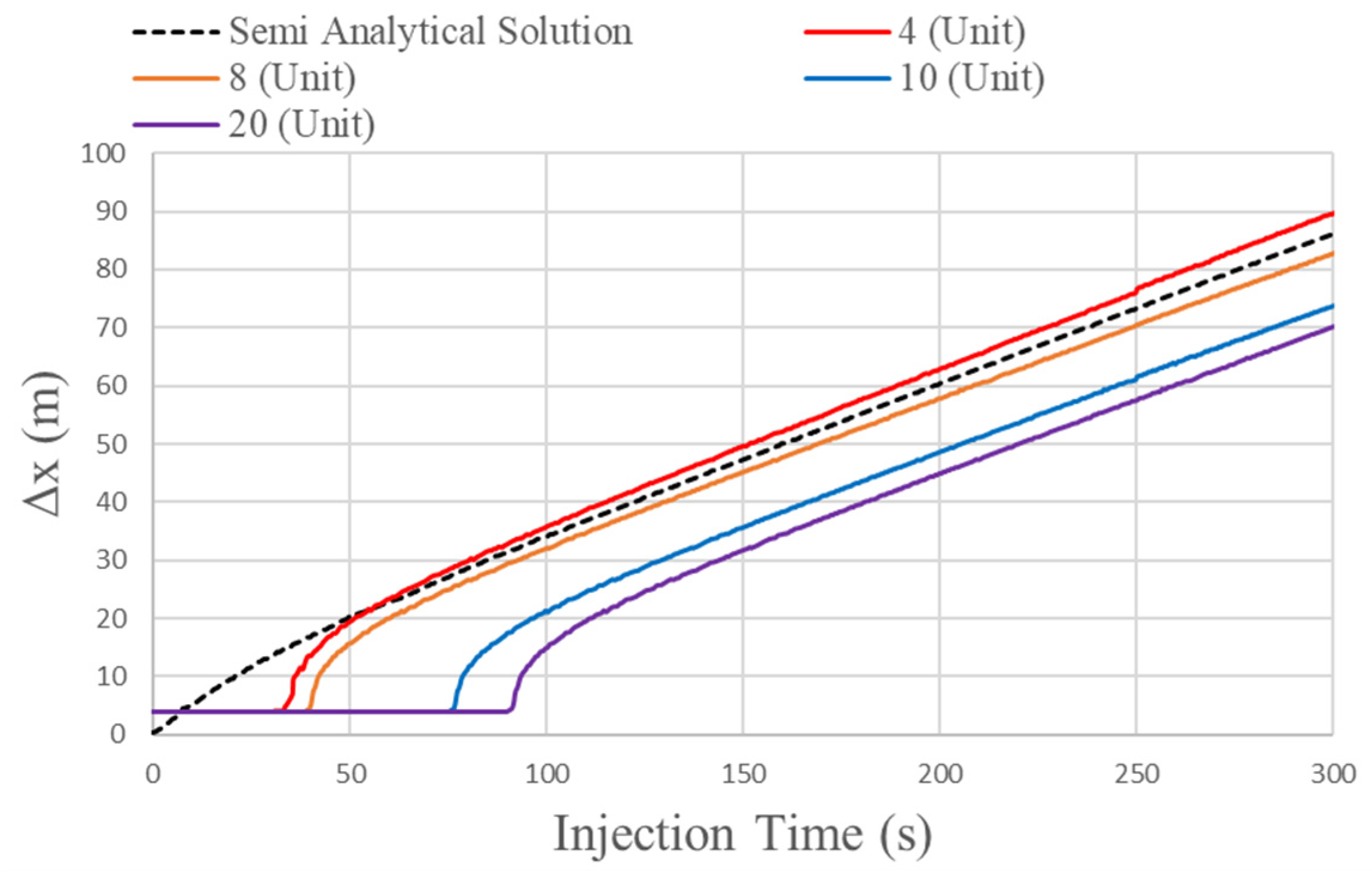
Figure 4 shows fracture half-lengths simulated by the MRST–phase-field model. To investigate the mesh sensitivity of the numerical model, the simulation was run for four different mesh sizes (4, 8, 10, and 20 units) being compared with the semi-analytical solution by [43]. The simulation results showed that it took a certain time for the fracture to start growing in the numerical simulation. Since the finite length of the initial fracture was assumed in the numerical model, it took some time to build up the pore pressure above the fracture propagation pressure in the domain. As shown in the figure, the deviation from the semi-analytical solution became smaller when a smaller mesh size was used. Overall, the numerical simulation results approached the semi-analytical solution with finer mesh sizes.
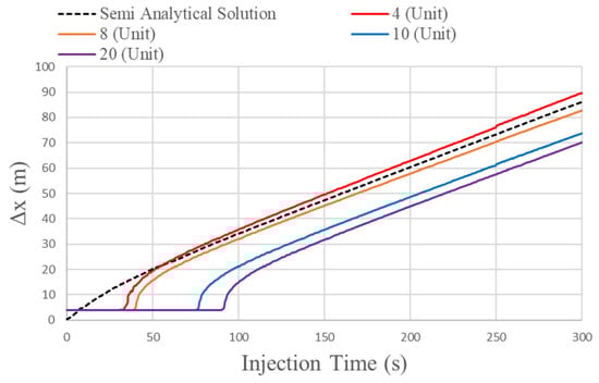
Figure 4.
Fracture half-length calculation results for different mesh sizes.
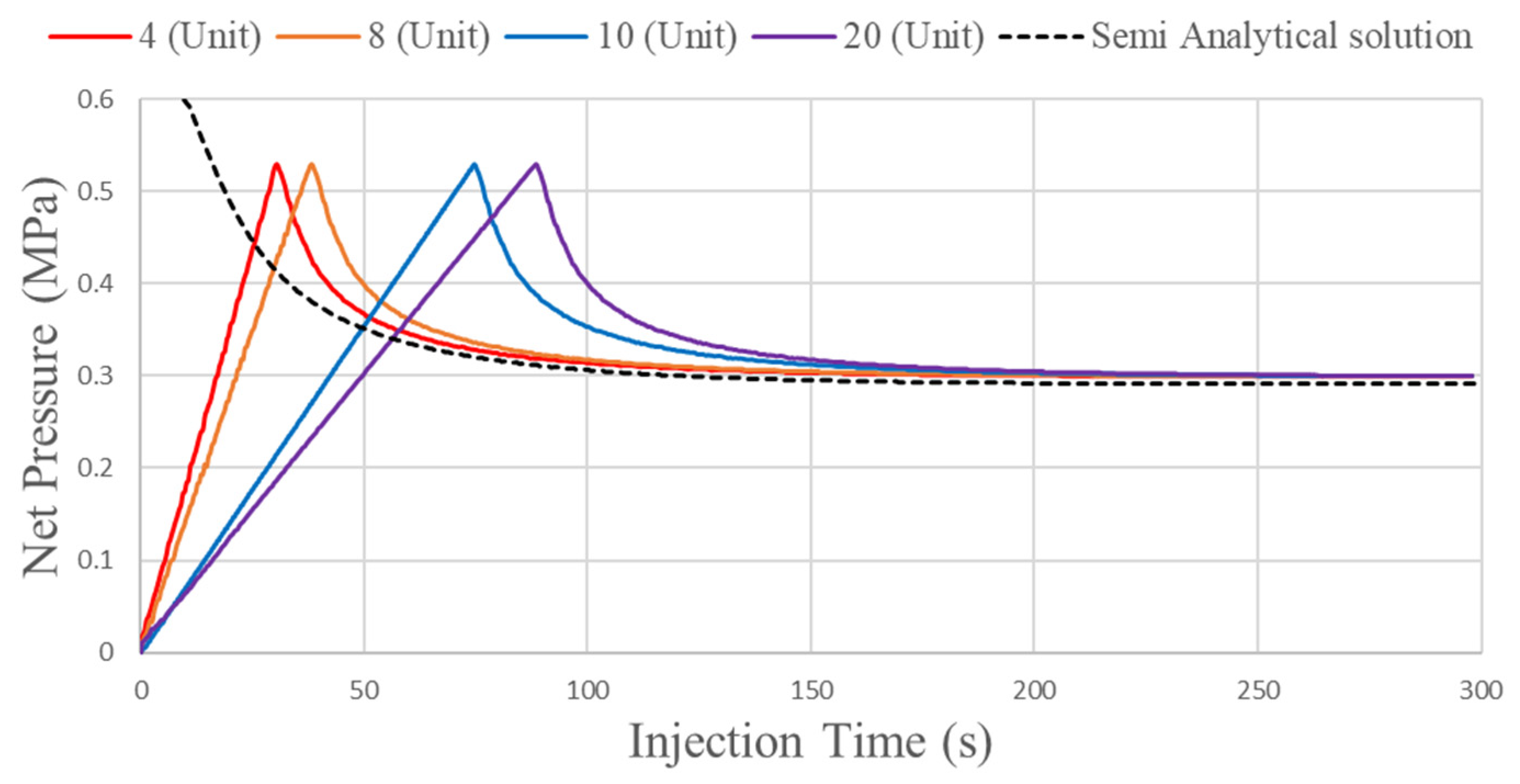
Figure 5 shows the net fracture pressure calculation results. The maximum fracture extension pressure were calculated by 0.529 MPa in the numerical models with different mesh sizes indicating that the initial fracture extension pressure was reasonably calculated by the numerical model and less dependent of the mesh size. On the other hand, the timing of the fracture breakdown is very sensitive to the mesh size. To overcome this discrepancy, a reasonably small mesh size should be employed. In this study, considering computational efficiency, a mesh size of 8 (unit) was selected for successive case studies.
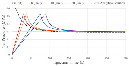
Figure 5.
Comparison of the critical pressure calculations with different mesh sizes.
2.6. Geometric and Numerical Model Division
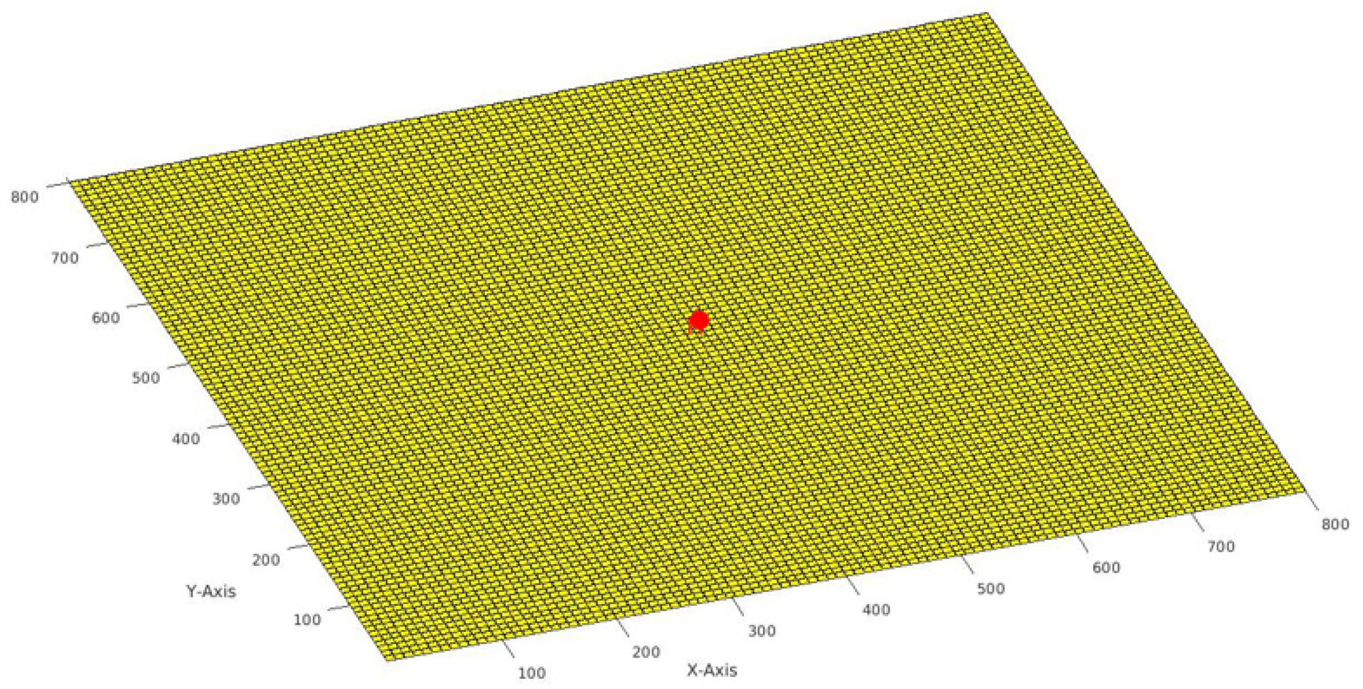
The following examples present four different scenarios for cold water injection into a geothermal reservoir. The simulations were conducted in a two-dimensional space with the element subdivision of 100 × 100, assuming granite-like properties. The case study used a vertical well drilled into the center of a homogeneous, isotropic reservoir (800 m × 800 m) (Figure 6).
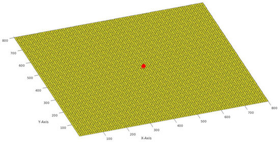
Figure 6.
Two-dimensional mesh geometry employed in the study (10,000 elements) and the location of the well (highlighted in red).
2.7. Model Parameters
This section details the assumptions and initial conditions for the simulations. The initial reservoir pressure and temperature were set at 8 MPa and 513 K, respectively. The simulations considered single-phase water flow, and the water was injected from a well with a constant injection rate of 0.7 m3/day per meter thickness of the reservoir until the initial fracture propagated.
2.8. Simulation Scheme
The simulations encompassed four scenarios: (1) hydro simulation, (2) hydromechanical simulation, (3) thermo-hydromechanical simulation, and (4) thermo-hydromechanical simulation with natural fractures. This section provides an overview of the methodology and procedures employed in each simulation scenario. Additional material properties used in the simulation are listed in Table 2.
Table 2.
Rock and fluid properties used in the case study.
In the thermo-hydro simulation performed by the modified MRST program, no flow boundaries were assumed at the outer boundaries of the reservoir. The no-flow condition was modeled by , while a constant temperature was assigned at the bottom boundaries. In the mechanical simulation performed by OpenGeoSys, in situ stresses were applied to the outer boundaries of the reservoir in a 2D plane strain condition.
3. Results
3.1. Case 1: Hydro Simulation
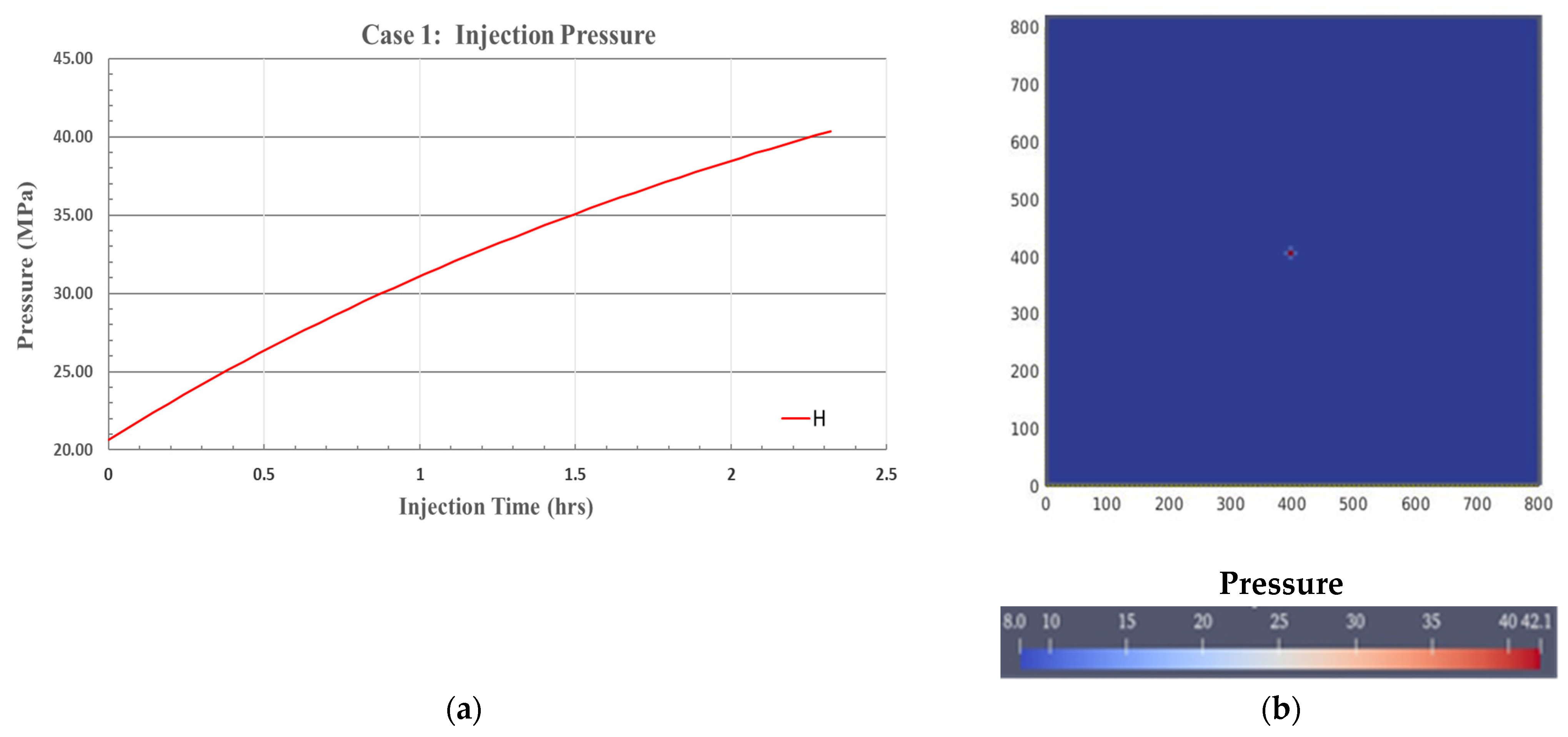
In this case, no thermal propagation or mechanical effects were considered. Figure 7 illustrates the bottom hole pressures of the injection well and the pressure distribution in the reservoir. As shown in Figure 7a, the injection pressure gradually increased as the water injection proceeded and reached a pressure of 40 MPa, which was above the minimum horizontal stress of 20 MPa. However, no fracture nucleated, because the mechanical effects were ignored in this case. The excess injection pressure dissipated radially in the near-wellbore vicinity, as illustrated in Figure 7b.
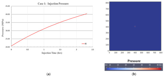
Figure 7.
(a) Pressure behavior during the simulation. (b) Pressure distribution after 0.7 m3 of injection.
3.2. Case 2: Hydromechanical Simulation
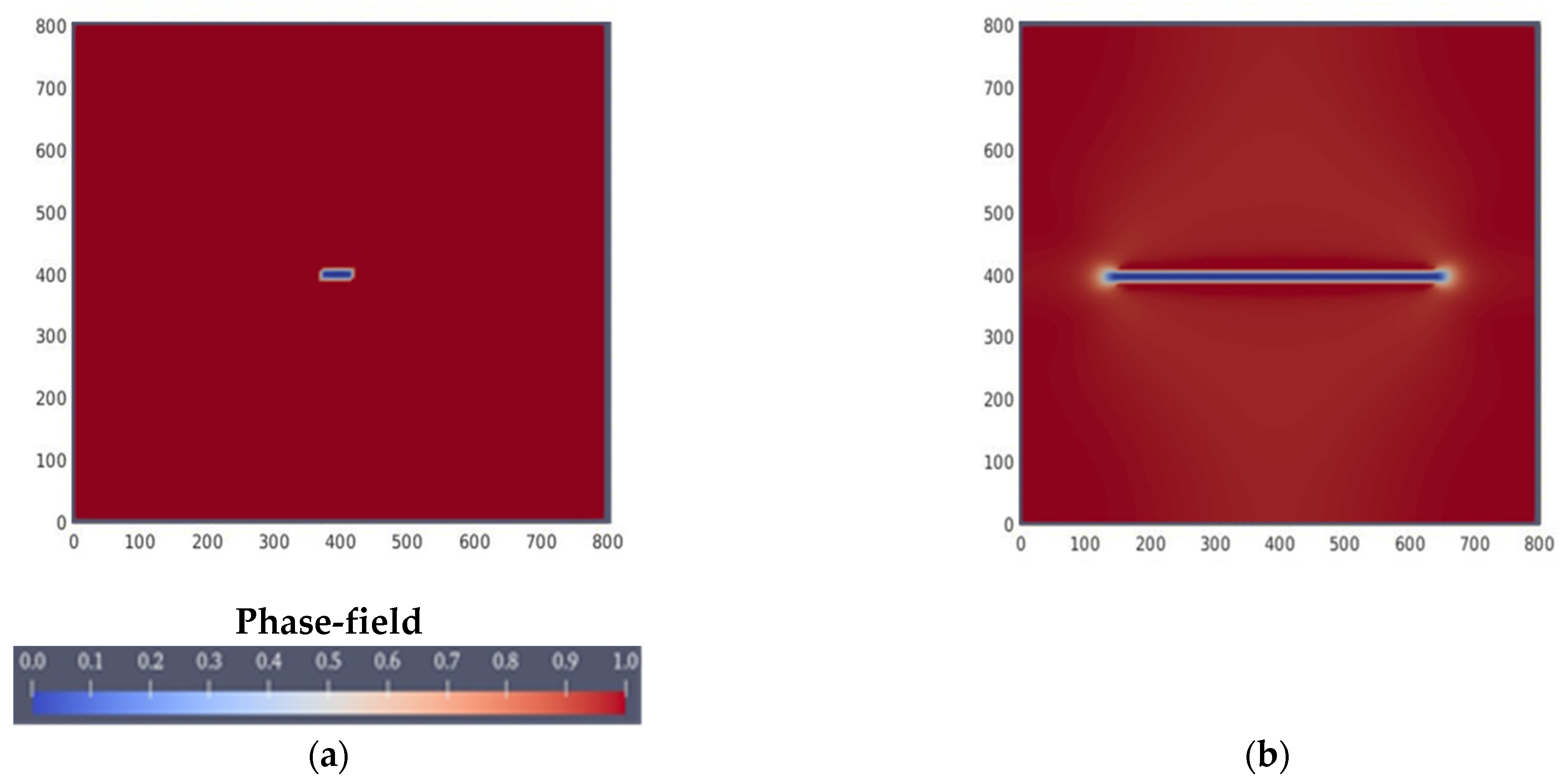
In this case, the hydro model (case 1) was coupled with a mechanical model to evaluate the effect of hydraulic fracturing in the EGS. A fracture with a length, , of 16 m was prescribed at the injection well in a direction parallel to the maximum horizontal stress (Figure 8).


Figure 8.
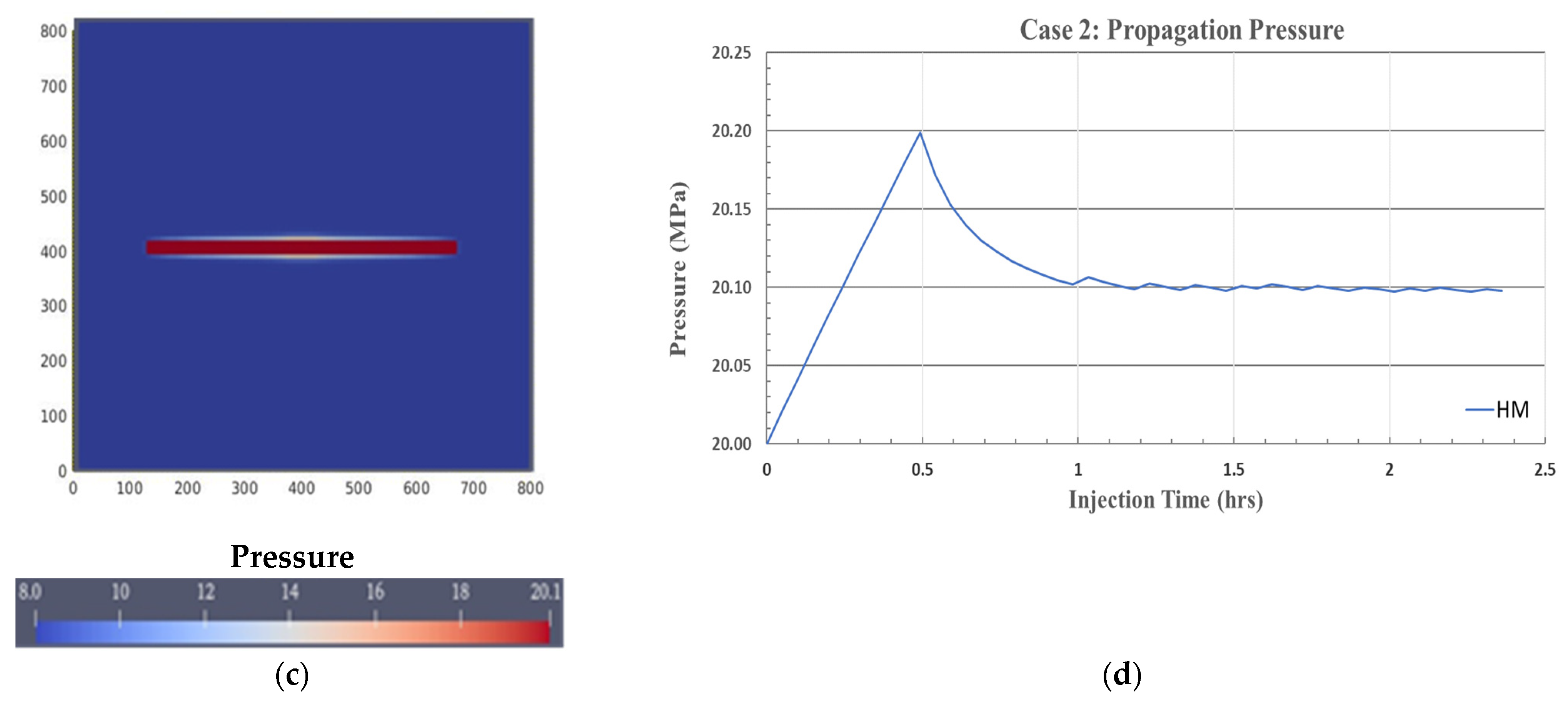
(a) The initial fracture location is represented by the phase-field profile. The 0 (blue) indicates a fully fractured rock, while the 1 (red) represents an unfractured rock. (b) Phase-field profile after 0.06 m3 of water injection. (c) Pore pressure distribution in the formation after 0.06 m3 of water injection. (d) Propagation pressure evolution at the injection well.
Once the phase-field value (v) was below 0.05, we considered the cell to be fractured and increased the cell permeability. The matrix and fracture permeabilities used in the computation of the scalar permeability multiplier defined in Equation (29) were assumed to be 100K mD and 1 mD, respectively.
Figure 8b shows the fracture propagation at an injection time of 2.4 h, while the pressure distribution around the fracture well is shown in Figure 8c. Figure 8d shows the injection pressure evolution in which the maximum pressure is attained at 20.198 MPa at 0.5 h. When leak-off is neglected, the critical fracture propagation pressure for a line crack in 2D is provided by
where is the critical pressure, is the fracture propagation pressure, and is the plane strain: Young’s modulus. The estimated maximum fracture propagation pressure from Equations (31) and (32) is 20.138 MPa, which is slightly lower than the simulated pressure of 20.198 MPa, and the final propagation fracture length is 248 m. Once the fracture propagates at approximately 0.5 h, the injection pressure starts to decline (Figure 8d).
3.3. Case 3: Thermo-Hydromechanical Simulation
In this example, thermal effects were considered to simulate injecting cold water into a hot reservoir. The initial reservoir temperature was assumed to be 513 K, whereas the temperature of the injected water was 413 K. To demonstrate the influence of temperature on fracture propagation, we created a cooling area along the initial crack, as shown in Figure 9b. The presence of a cooling area can influence the fracture pattern of a material. Cooling can cause thermal stresses within the material, which can result in a secondary fracture occurring in a direction different from the main fracture (Figure 9a), and this can also be seen in the pressure distribution (Figure 9c). As shown in Figure 9d, the maximum injection pressure was 20.12 MPa, which is lower than that of case 2 (20.19 MPa).
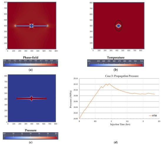
Figure 9.
Case 3: (a) The phase-field profile at t = 2.4 h indicates the presence of a secondary fracture in a different direction than that of the main fracture. (b) Temperature distribution at 2.4 h. (c) Pore pressure distribution in the formation. (d) Pressure behavior at the injection well.
3.4. Case 4: Thermo-Hydromechanical Simulation in a Naturally Fractured Formation
This study investigated the interaction between pre-existing (i.e., natural) fractures and hydraulic fractures. It was assumed that the two natural fractures were oriented in a north–south direction, as shown in Figure 10a. An injection well was drilled between the two natural fractures, and the distance between the natural fracture and the well was 96 m. Other rocks and fluid properties were the same as in the previous cases. The fracture propagation was symmetrical toward the x-axis (x+ and x−). When the hydraulic fracture hit the natural fractures, the hydraulic fracture branched to the natural fractures, as shown in Figure 10b. Figure 10c,d show the pressure and temperature distributions in the formation, respectively. As shown in Figure 10e, the maximum injection pressure was 20.114 MPa, and the final propagation fracture was 168 m, which is lower than in case 3.
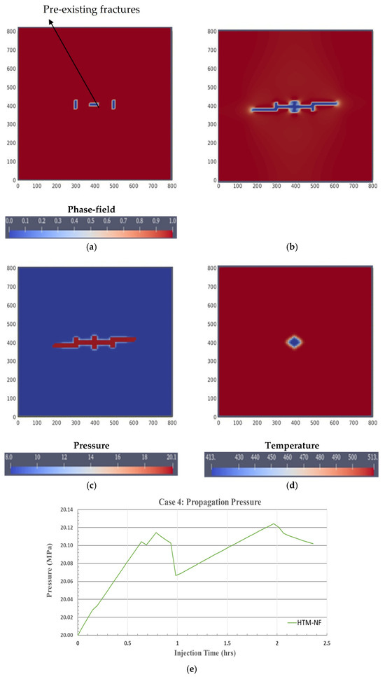
Figure 10.
(a) Location of the initial and natural (pre-existing) fractures. (b) The interaction between the hydraulics and natural fractures is illustrated by the phase-field model. (c) Pore pressure distribution at t = 2.4 h. (d) Temperature distribution in the formation at t = 2.4 h. (e) Pressure behavior at the injection well.
The possible orientations of natural fractures when interacting with hydraulic fractures include arrest, crossing, and branching at the tips of natural fractures [12]. In case 4, referred to as branches and crosses at the end of NF (Figure 10), this phenomenon occurs when the hydraulic fracture diverges and extends into the natural fracture. This signifies that the hydraulic fracture deviates from its original propagation direction and infiltrates the natural fracture at its end point. As a result, the hydraulic fracture effectively traces the pathway of the natural fracture, progressing within its confines. It is crucial to acknowledge that the orientation of the natural fractures can exert a significant influence on the propagation behavior of the hydraulic fracture, thereby imparting distinct characteristics to the resulting fracture geometry. The specific impact of each orientation depends on factors such as the orientation and properties of the natural fractures, the stress conditions, and the geomechanical behavior of the rocks. Understanding these impacts is crucial for optimizing the design and implementation of hydraulic fracturing operations.
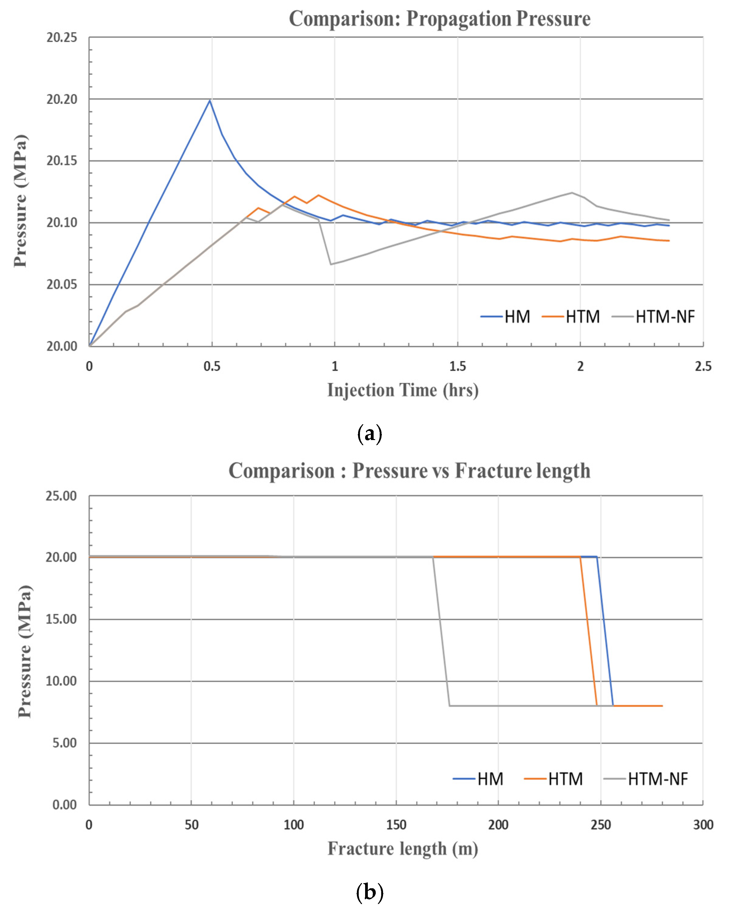
In Figure 11a, the injection pressures of three different cases (cases 2, 3, and 4) were compared. In case 2, where temperature effects were not considered, the injection pressure required to reach the critical pressure was the highest between the three cases at 20.19 MPa and occurred the fastest at 0.5 h. Additionally, the longest fracture length of 248 m occurred in this case. On the other hand, in case 4, where both temperature effects and natural fractures were considered, the injection pressure required to reach the critical pressure was the lowest between the three cases at 20.11 MPa and was the shortest at 168 m because of the interaction with the natural fracture.
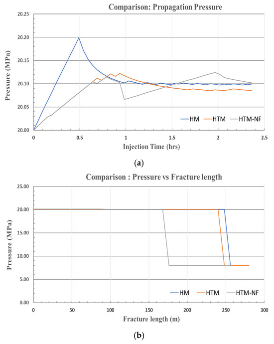
Figure 11.
(a) Comparison of the propagation pressures. (b) Comparison of pressure and fracture length.
4. Discussion
This simulation can handle fluid properties that depend on pressure and temperature changes and can handle interactions between hydraulics and natural fractures. The MRST and OGS (OpenGeoSys) simulation results regarding the influence of the hydraulic fracture, thermal effects, and natural fracture on the EGS are as follows.
The first result is related to the hydraulic fracture. When water was injected into the reservoir, the pressure in the fracture created around the injection well gradually increased until it reached the fracture propagation pressure (). This led to an increase in the fracture length (Figure 7b) and improved the well injectivity, resulting in lower injection pressures.
The second result is related to thermal effects. To demonstrate the significant influence of temperature on fracture propagation, it is important to create a cooling area along the initial crack. The presence of a cooling area (Figure 8b) can lead to secondary fractures opening (Figure 8a) in directions perpendicular to the main fractures. The presence of a cooling area can lower the critical pressure required to induce fractures during cold-water injection, which is due to the influence of temperature changes on the thermal strain. This effect was proportional to the temperature change (ΔT) and the coefficient of thermal expansion (α) of the rock. The cooling region caused the injection water pressure to reach the propagation pressure (), and the fracture propagation was lower than in case 2 without considering the temperature at 0.7 h (Figure 11a). Considering the thermal effect, the length of the main crack became shorter. This was because the secondary fracture formed perpendicular to the direction of the initial crack, requiring an additional water injection to fill it (Figure 11b). According to Perkins and Gonzalez [41], injecting lower-temperature fluid into a reservoir gradually forms a cooling area around the well (Figure 8b). The effective stress ) around the cooling area was corrected because of the additional effect of thermal strain . The relationship between the effective stress and the total stress ) in the porous media (Equation (10)) resulted in a decrease in the temperature leading to total stress reduction (Figure 11). This was the result of plotting the injection pressure at the wellbore during the simulation. The influence of changes in the water viscosity and density caused a significant pressure difference (∆p) between the pressure at the wellbore and the fracture tip. The final fracture propagation lengths of case 2 (HM) and case 3 (HTM) were 248 m and 240 m, respectively. In case 2, the fracture tip pressure was 20.19 MPa, while in case 3, it was 20.12 MPa. Therefore, case 3 had a lower hydraulic fracture than case 2. This result showed that the temperature had a significant impact on improving the fracture propagation.
The third result is related to the natural fracture. In case 4, the fracture length was the shortest at 168 m compared with the other cases. The interaction between injection pressure and natural pressure is an important consideration in hydraulic fracturing. When a natural fracture is perpendicular to the direction of the hydraulic fracture, it can act as a barrier and cause the hydraulic fracture to stop growing. The orientation of the natural fractures played a significant role in the interaction with hydraulic fractures. In the specific case studied, where the natural fractures were oriented in the y-axis (y+ and y−), the hydraulic fractures branched out when they encountered these pre-existing fractures. This branching behavior resulted in a deviation from the original fracture propagation path. The interaction between the hydraulic fractures and the natural fractures had implications for the overall process. The branching of hydraulic fractures into natural fractures influenced the pressure and temperature distributions in the formation. It also affected the maximum injection pressure and the distance of fracture propagation. As such, in case 4, the lowest injection pressure required to reach the critical pressure, of 20.12 MPa, was observed when considering the interaction in the natural fracture during hydraulic fracturing, as shown in Figure 11a. However, once the interaction was complete and additional fractures were created, the required injection pressure tended to gradually increase, up to 20.124 MPa. This was likely due to the need for more injected fluid to fill up the entire volume of the newly created natural fracture to continue the fracturing process.
Future research can focus on characterizing the behavior of different types of natural fractures, their orientations, and their influence on fracture propagation paths. This understanding can contribute to more effective reservoir management and optimization of geothermal energy extraction.
5. Conclusions
In this study, a two-way coupling technique for thermo-hydromechanical modeling was used to simulate hydraulic fracture propagation in an EGS using the phase-field approach. The simulation results demonstrate the importance of noting geomechanical effects on injection performance during cold-water injections into high-temperature reservoirs, especially when the water injection pressure exceeds the fracturing pressure of the rock. To account for fracturing effects, one must not neglect thermoelastic effects and the presence of natural fractures (if any). Hydraulic fracture interactions between natural fractures and cold-water injections stimulate fracture propagation. The phase-field approach was utilized to simulate hydraulic fracture propagation in an enhanced geothermal system (EGS).
Author Contributions
Conceptualization, V.P. and K.F.; methodology, V.P.; software, V.P.; validation, V.P. and K.F.; formal analysis, V.P.; investigation, V.P.; resources, V.P.; data curation, V.P. and K.F.; writing—original draft preparation, V.P.; writing—review and editing, K.F.; visualization, V.P.; supervision, K.F.; project administration, V.P. All authors have read and agreed to the published version of the manuscript.
Funding
This work was supported by the research grant of Arai Foundation.
Data Availability Statement
The data are available from the corresponding author upon reasonable request.
Acknowledgments
Part of the present work was performed as part of the activities of the Research Institute of Sustainable Future Society, Waseda Research Institute for Science and Engineering, Waseda University.
Conflicts of Interest
The authors declare no conflict of interest.
Nomenclature
| X | Distance (m) |
| Δt | Time interval (s) |
| E | Young’s modulus (GPa) |
| v | Poisson’s ratio |
| Fracture toughness (Pa·m) | |
| Φ | Porosity |
| Fluid source terms () | |
| µ | Fluid viscosity (Pa·s) |
| Bulk modulus fluid (GPa) | |
| b | Body force (N/kg) |
| τ | External forces (N) |
| Effective stress (Pa) | |
| Rock density (kg/) | |
| Water density (kg/) | |
| Water viscosity (Pa·s) | |
| Average thermal conductivity (W/(m·K) | |
| Specific heat of fluid (J/kg) | |
| Specific internal energy (KJ/kg) | |
| Porosity compressibility (/Pa) | |
| β | Thermal expansion (°C) |
References
- Shere, J. Renewable: The World—Changing Power of Alternative Energy; St. Martin’s Press: New York, NY, USA, 2013. [Google Scholar]
- IRENA. Renewable Capacity Statics 2018; International Renewable Energy Agency (IRENA): Abu Dhabi, United Arab Emirates, 2018. [Google Scholar]
- Tiwari, G.N.; Ghosal, M.K. Renewable Energy Resources: Basic Principles and Applications; Alpha Science Int’l Ltd.: New Delhi, India, 2005. [Google Scholar]
- Gudmundsson, G.H. Transmission of basal variability to a glacier surface. J. Geophys. Res. Solid Earth 2003, 108, 1–19. [Google Scholar] [CrossRef]
- Batchelor, A.S. The Stimulation of a Hot Dry Rock Geothermal Reservoir in the Cornubian Granite, England. In Proceedings of the Eighth Workshop Geothermal Reservoir Engineering, Cornwall, UK, 1 January 1982. [Google Scholar]
- Kelkar, S.; Lewis, K.; Hickman, S.; Davatzes, N.; Moos, D.; Zyvoloski, G. Modeling Coupled Ther-mal-Hydrological-Mechanical Processes During Shear Stimulation of an EGS Well. In Proceedings of the Thirty-Seventh Workshop on Geothermal Reservoir Engineering, Stanford, CA, USA, 30 January–1 February 2012; Volume 1988, pp. 1–8. [Google Scholar]
- Tester, J.W.; Anderson, B.J.; Batchelor, A.S.; Blackwell, D.D.; DiPippo, R.; Drake, E.M.; Garnish, J.; Livesay, B.; Moore, M.C.; Nichols, K.; et al. Impact of enhanced geothermal systems on US energy supply in the twenty-first century. Philos. Trans. R. Soc. A Math. Phys. Eng. Sci. 2007, 365, 1057–1094. [Google Scholar] [CrossRef] [PubMed]
- Zoback, M.D. Reservoir Geomechanics; Cambridge University Press: Cambridge, MA, USA, 2007. [Google Scholar] [CrossRef]
- Adachi, J.; Siebrits, E.; Peirce, A.; Desroches, J. Computer simulation of hydraulic fractures. Int. J. Rock Mech. Min. Sci. 2007, 44, 739–757. [Google Scholar] [CrossRef]
- Yi, G.; Yu, T.; Bui, T.Q.; Ma, C.; Hirose, S. SIFs evaluation of sharp V-notched fracture by XFEM and strain energy approach. Theor. Appl. Fract. Mech. 2017, 89, 35–44. [Google Scholar] [CrossRef]
- Zarrinzadeh, H.; Kabir, M.; Varvani-Farahani, A. Static and dynamic fracture analysis of 3D cracked orthotropic shells using XFEM method. Theor. Appl. Fract. Mech. 2020, 108, 102648. [Google Scholar] [CrossRef]
- McClure, M.; Babazadeh, M.; Shiozawa, S.; Huang, J. Fully coupled hydromechanical simulation of hydraulic fracturing in three-dimensional discrete fracture networks. Soc. Pet. Eng.-SPE Hydraul. Fract. Technol. Conf. 2016, 21, 1302–1320. [Google Scholar] [CrossRef]
- Gu, H.; Weng, X. Criterion for fractures crossing frictional interfaces at non-orthogonal angles. In Proceedings of the 44th U.S. Rock Mechanics Symposium and 5th U.S.-Canada Rock Mechanics Symposium, Salt Lake City, UT, USA, 27 June 2010. [Google Scholar]
- Bourdin, B.; Francfort, G.; Marigo, J.-J. Numerical experiments in revisited brittle fracture. J. Mech. Phys. Solids 2000, 48, 797–826. [Google Scholar] [CrossRef]
- Francfort, G.; Marigo, J.-J. Revisiting brittle fracture as an energy minimization problem. J. Mech. Phys. Solids 1998, 46, 1319–1342. [Google Scholar] [CrossRef]
- Alessi, R.; Marigo, J.-J.; Maurini, C.; Vidoli, S. Coupling damage and plasticity for a phase-field regularisation of brittle, cohesive and ductile fracture: One-dimensional examples. Int. J. Mech. Sci. 2018, 149, 559–576. [Google Scholar] [CrossRef]
- Carrara, P.; Ambati, M.; Alessi, R.; De Lorenzis, L. A framework to model the fatigue behavior of brittle materials based on a variational phase-field approach. Comput. Methods Appl. Mech. Eng. 2019, 361, 112731. [Google Scholar] [CrossRef]
- Bourdin, B.; Chukwudozie, C.P.; Yoshioka, K. A Variational Approach to the Numerical Simulation of Hydraulic Fracturing. Proc.-SPE Annu. Tech. Conf. Exhib. 2012, 2, 1442–1452. [Google Scholar] [CrossRef]
- Hofacker, M.; Miehe, C. Continuum phase field modeling of dynamic fracture: Variational principles and staggered FE implementation. Int. J. Fract. 2012, 178, 113–129. [Google Scholar] [CrossRef]
- Wick, T.; Singh, G.; Wheeler, M.F. Fluid-Filled Fracture Propagation With a Phase-Field Approach and Coupling to a Reservoir Simulator. SPE J. 2016, 21, 0981–0999. [Google Scholar] [CrossRef]
- Wilson, Z.A.; Landis, C.M. Phase-field modeling of hydraulic fracture. J. Mech. Phys. Solids 2016, 96, 264–290. [Google Scholar] [CrossRef]
- Heider, Y.; Markert, B. Simulation of hydraulic fracture of porous materials using the phase-field modeling approach. Pamm 2016, 16, 447–448. [Google Scholar] [CrossRef]
- Chukwudozie, C.; Bourdin, B.; Yoshioka, K. A variational phase-field model for hydraulic fracturing in porous media. Comput. Methods Appl. Mech. Eng. 2019, 347, 957–982. [Google Scholar] [CrossRef]
- Zhou, S.; Zhuang, X.; Rabczuk, T. Phase-field modeling of fluid-driven dynamic cracking in porous media. Comput. Methods Appl. Mech. Eng. 2019, 350, 169–198. [Google Scholar] [CrossRef]
- Yoshioka, K.; Yoshioka, K.; Bourdin, B.; Bourdin, B. A variational hydraulic fracturing model coupled to a reservoir simulator. Int. J. Rock Mech. Min. Sci. 2016, 88, 137–150. [Google Scholar] [CrossRef]
- Olasolo, P.; Juárez, M.; Morales, M.; D’amico, S.; Liarte, I. Enhanced geothermal systems (EGS): A review. Renew. Sustain. Energy Rev. 2016, 56, 133–144. [Google Scholar] [CrossRef]
- Xia, Y.; Plummer, M.; Podgorney, R.; Ghassemi, A. An Assessment of Some Design Constraints on Heat Production of a 3D Conceptual EGS Model Using an Open-Source Geothermal Reservoir Simulation Code. In Proceedings of the Forty-First Workshop on Geothermal Reservoir Engineering, Stanford University, Stanford, CA, USA, 22–24 February 2016. [Google Scholar]
- Hu, L.; Winterfeld, P.H.; Fakcharoenphol, P.; Wu, Y.-S. A novel fully-coupled flow and geomechanics model in enhanced geothermal reservoirs. J. Pet. Sci. Eng. 2013, 107, 1–11. [Google Scholar] [CrossRef]
- Haris, M.; Hou, M.Z.; Feng, W.; Luo, J.; Zahoor, M.K.; Liao, J. Investigative Coupled Thermo-Hydro-Mechanical Modelling Approach for Geothermal Heat Extraction through Multistage Hydraulic Fracturing from Hot Geothermal Sedimentary Systems. Energies 2020, 13, 3504. [Google Scholar] [CrossRef]
- Pandey, S.; Chaudhuri, A.; Kelkar, S. A coupled thermo-hydro-mechanical modeling of fracture aperture alteration and reservoir deformation during heat extraction from a geothermal reservoir. Geothermics 2016, 65, 17–31. [Google Scholar] [CrossRef]
- Rinaldi, A.P.; Rutqvist, J.; Sonnenthal, E.L.; Cladouhos, T.T. Coupled THM modeling of hydroshearing stimulation in tight fractured volcanic rock. Transp. Porous Media 2015, 108, 131–150. [Google Scholar] [CrossRef]
- Xie, L.; Min, K.B. Initiation and propagation of fracture shearing during hydraulic stimulation in enhanced geothermal system. Geothermics 2016, 59, 107–120. [Google Scholar] [CrossRef]
- Yuan, Y.; Xu, T.; Moore, J.; Lei, H.; Feng, B. Coupled thermo–hydro–mechanical modeling of hydro-shearing stimulation in an enhanced geothermal system in the raft river geothermal field, USA. Rock Mech. Rock Eng. 2020, 53, 5371–5388. [Google Scholar] [CrossRef]
- Li, S.; Zhang, D. Three-Dimensional Thermoporoelastic Modeling of Hydrofracturing and Fluid Circulation in Hot Dry Rock. J. Geophys. Res. Solid Earth 2023, 128, e2022JB025673. [Google Scholar] [CrossRef]
- Krogstad, S.; Lie, K.A.; Møyner, O.; Nilsen, H.M.; Raynaud, X.; Skaflestad, B. MRST-AD—An Open-Source Framework for Rapid Prototyping and. In Proceedings of the SPE Reservoir Simulation Symposium, Houston, TX, USA, 23–25 February 2015. [Google Scholar]
- Yoshioka, K.; Parisio, F.; Naumov, D.; Lu, R.; Kolditz, O.; Nagel, T. Comparative verification of discrete and smeared numerical approaches for the simulation of hydraulic fracturing. GEM—Int. J. Geomath. 2019, 10, 13. [Google Scholar] [CrossRef]
- Griffith, A.A., VI. The phenomena of rupture and flow in solids. Philos. Trans. R. Soc. Lond. Ser. A 1921, 221, 163–198. [Google Scholar]
- Bourdin, B.; Francfort, G.A.; Marigo, J.-J. The Variational Approach to Fracture. J. Elast. 2008, 91, 5–148. [Google Scholar] [CrossRef]
- Faust, C.R.; Mercer, J.W. Geothermal reservoir simulation: 2. Numerical Solution Technique for Liquid- and Vapor-Dominated Hydrothermal Systems. Water Resour. Res. 1979, 15, 31–46. [Google Scholar] [CrossRef]
- Coats, K.H. Geothermal Reservoir Modeling. In Proceedings of the SPE Annual Fall Technical Conference and Exhibition, Denver, CO, USA, 9–12 October 1977. [Google Scholar]
- Al-Shemmeri, T.T. Engineering Fluid Mechanics Solution Manual; Bookboon: London, UK, 2012. [Google Scholar]
- Praditia, T.; Helmig, R.; Hajibeygi, H. Multiscale formulation for coupled flow-heat equations arising from single-phase flow in fractured geothermal reservoirs. Comput. Geosci. 2018, 22, 1305–1322. [Google Scholar] [CrossRef]
- Garagash, D.I. Plane-strain propagation of a fluid-driven fracture during injection and shut-in: Asymptotics of large toughness. Eng. Fract. Mech. 2006, 73, 456–481. [Google Scholar] [CrossRef]


Disclaimer/Publisher’s Note: The statements, opinions and data contained in all publications are solely those of the individual author(s) and contributor(s) and not of MDPI and/or the editor(s). MDPI and/or the editor(s) disclaim responsibility for any injury to people or property resulting from any ideas, methods, instructions or products referred to in the content. |
© 2023 by the authors. Licensee MDPI, Basel, Switzerland. This article is an open access article distributed under the terms and conditions of the Creative Commons Attribution (CC BY) license (https://creativecommons.org/licenses/by/4.0/).