Abstract
Since existing energy system models often represent storage behavior in a simplified way, in this work, a tool chain for deriving consistent storage model parameters for optimization models is developed. The aim of our research work is to identify what are non-negligible influences on the the technical characteristics and dynamic behavior of the storage, to quantify the effect of these influences, and represent these effects in the model. This paper describes the developed tool chain and presents its application using an example. The tool chain consists of the steps “parameter screening”, “dynamic simulation”, “regression analysis” and “refining optimization model”. It is investigated which parameters have an influence on the storage system (here pumped hydroelectric energy storage (PHES)), how the storage behavior is modeled, which influencing factors have a measurable effect on the system, and how these findings can be integrated into optimization models. The main finding is that in the case of PHES, the dependency of the charging and discharging efficiency on the power is significant, but no further influencing factor has to be considered for accurate modeling (0.946 ≤ R2 ≤ 0.988) of the efficiency. It is concluded that the presented toolchain is suitable for other storage technologies as well, including the analysis of aging behavior.
1. Introduction
The participants of Glasgow Climate Pact COP26 reaffirmed “the Paris Agreement temperature goal of holding the increase in the global average temperature to well below 2 C above pre-industrial levels and pursuing efforts to limit the temperature increase to 1.5 C above pre-industrial levels” [1]. To achieve this goal, it is necessary to switch from mostly fossil fuels in energy generation to renewable energy sources. This means current energy systems have to be changed massively with respect to their energy generation technologies. One way to analyze which technologies suit the challenge best and to determine how much and where to build them is to use national and transnational energy system models. These energy system models optimize the operation and the installation of energy generation. Examples of this type of model are TIMES [2], REMix [3], and Calliope [4].
Besides energy generation technologies, the energy system models also include energy storage systems as a way to balance demand and generation. Most commonly, the storage technologies are represented by their power, storage capacity, and efficiency, all of which are typically modeled as constant over the optimization horizon (e.g., [5]).
This way of modeling does not represent the real behavior of storage systems though. To name some examples: The efficiency and available storage capacity of a Li-Ion battery depend highly on its age. Another example is the dependency of mechanical storage, such as compressed air energy storage (CAES) or pumped hydroelectric energy storage (PHES), on the mass flow rates of air and water, respectively, which again depend on the required charging or discharging power of the storage operation. Redox Flow batteries are another example to operate with up to 1.5 times their nominal power, but only for a limited time.
The reason for failing to present these features of storage systems in energy system models so far is that storage systems are just one part of the energy system, and modeling it in a more detailed way leads to a higher computational burden. These simplifications are acceptable (and necessary) as long as energy storage plays only a small role in the system, and allows us to estimate the amount of storage needed in general. However, recent global events showed, that energy storage systems will play a more significant role in future energy systems. This bears the question of how great is the need for storage exactly and how much of each of the different storage technologies will be needed. To answer these questions, it is necessary to represent the different technologies in a more detailed way. The ever increasing available computational power supports this and enables having more detailed models without highly increasing runtimes.
Here, the modeling of energy storage in transnational energy system models can learn from already existing more detailed models that analyze the operation of electric storage devices in local energy systems or that have been created for the purpose of technology development (e.g., [6,7,8,9,10,11,12]). For this reason, the IEA Annex 32 “Open Sesame - Modelling of energy storages for simulation/optimization of energy systems” is carried out to promote the transfer of knowledge between modelers of energy storage systems at different levels of detail. The presented results were developed within the framework of the annex, respectively, within the framework of the associated R&D project “Sesame Seed” [FKZ 03EI1021].
To rely on a classified differentiation between energy storage models, four different levels, according to their level of detail, are defined in Sesame Seed. So-called “Level 3” models stand for very detailed dynamic simulation models of specific storage technologies, which, for example, model physical, thermodynamic and chemical effects in depth. On the other hand, there are transnational energy system models that model energy storage technologies in a very simplified way (“Level 0” models). Table 1 gives an abridged overview of this model classification.

Table 1.
Classification of energy storage models considering model application and modelling depth.
Our literature research has shown that many transnational energy system models used in recent years are at level 0 [2,3,5,13].
Future investigations of energy storage requirements are to be carried out with level 1 energy system models due to the increasing importance of energy storage systems described above. Based on the literature, there seems to lack publications that present a systematic method for evaluation of the recommended modeling depth for energy storages. Against this background, this paper aims at closing this gap and presenting a tool chain that systematically derives from dynamic simulation models on level 3, which level of detail will be recommended for the modeling of energy storage devices in transnational energy system models on level 1 in the future.
Our developed tool chain supports users in developing accurate representations of their selected energy storage system in available or to-be-designed energy system optimization models. This tool chain aspires to construct simple, yet highly informative storage system representations from the ground up. As each step is full of optional steps to be taken and could be left out entirely (if desired), this workflow can be tailored to any user’s needs. Within the following pages, we will explain each step of the chain individually (Section 2), before exemplifying the application of the tool chain for the charging process of pumped hydro energy storage only in Section 3. The paper then concludes with Section 4 discussing and evaluating the insights gathered throughout developing this tool chain and applying it for pumped-storage hydroelectric systems and adiabatic compressed-air electric storage systems (results presented in future publications).
2. Materials and Methods
As described in the introduction, it is recommended to model future energy storage technologies in more detail in transnational energy system models. Nevertheless, limiting computing power has to be taken into account, which is why significant mathematical simplifications are still necessary compared to the modeling of energy storage systems in very detailed dynamic simulation models. The developed tool chain guides the user from screening potentially important physical and technological parameters (input electrical power, storage duration, etc.) for a highly accurate level 3 energy storage model to extract the most relevant components and information of such level 3 models to the desired level of simplicity (level 2 or level 1 models) using statistical tools which can be tailored to the user’s needs. The tool chain consists of four crucial steps, which are thoroughly explained in the following sections. A general workflow of these four steps is illustrated in Figure 1.

Figure 1.
Tool chain to identify most influencing factors concerning the charging, storage, and discharging process.
This section will conceptually introduce the four core steps of the developed tool chain. The first step “Screening parameters” (Section 2.1) serves to identify physical and technological factors, such as storage unit capacity or storage duration, whose variability is assumed to have an impact on system outputs relevant to the user (e.g., storage unit efficiency, changing states of charge, etc.). Having obtained a list of potentially influencing factors, the second step “Dynamic simulation” (Section 2.2) will focus on designing a physically accurate level 3 model, representing the changes of the desired outputs by varying the selected factors as closely as possible. This step also contains recommendations on experimental designs for obtaining a large data set, representing the level 3 model. This data set is fundamental for step 3 “Regression analysis”, explained in Section 2.3. The explained regression analysis aims to convert the obtained information about the predictions by the level 3 model into level 2 or level 1 surrogate models. By adjusting the complexity of the regression model to the wanted predictive accuracy, and available computational power, our tool chain allows for a flexible integration of the level 2 or level 1 model into existing energy system optimization models (step 4 “Refining optimization model”; Section 3.4). Again, all operations of the individual steps can be adjusted to the user’s needs, and not all operations are mandatory.
2.1. Step 1: Screening Parameters
As described in the previous section, the first step of the tool chain is the screening of parameters. This step is important to obtain a representation as complete as possible of the technology under investigation and to consider all system input and system output for both simulations (cf. Section 3.2.1) and modeling of energy storages in energy system models (cf. Section 3.4). By screening the parameters, the aim is to identify influential parameters affecting the system output and identifying relevant system output [14]. It is necessary to perform methodical, structured considerations to ensure finding as many parameters as possible. The reason for considering the parameters is that with more parameters taken into account, the system descriptions by the simulation model and the experimental design will become more congruent with the occurring process.
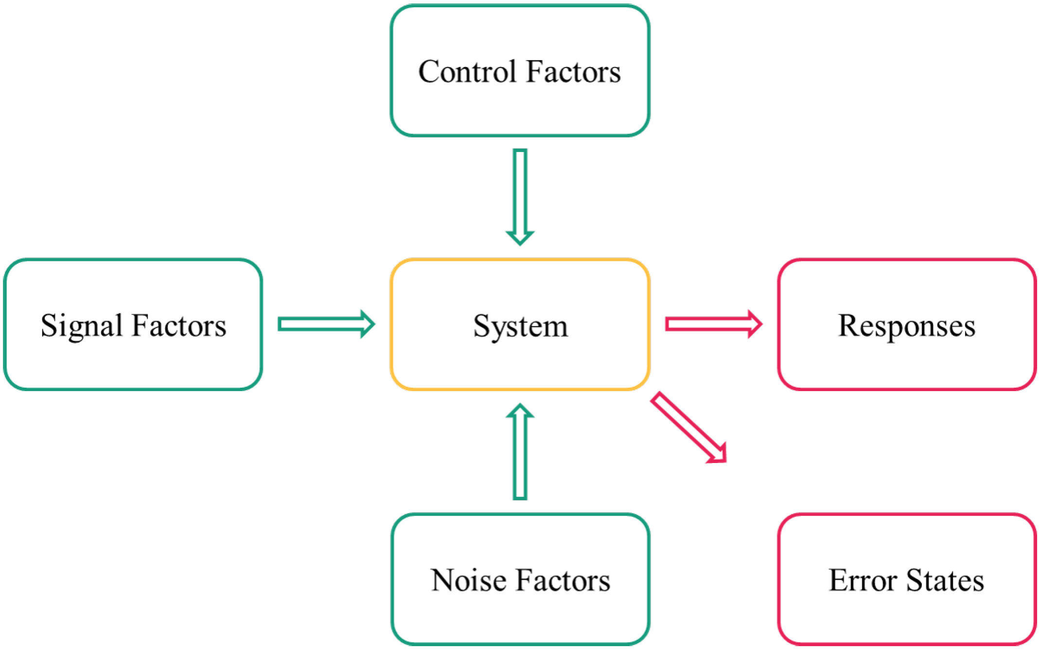
A helpful method is the parameter diagram which has its origins in Robust Design. Besides the preparation of the experimental design, the parameter diagram also serves the general understanding of the system. All parameters included in the experimental design are called factors, while all other parameters not included in the experimental design should be kept constant [14]. As shown in Figure 2, the parameter diagram includes control, signal, and noise factors affecting the system, as well as system results which are called either responses or error states. While the responses are desired system outputs, the error states are designated as undesired outputs [14].
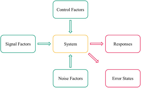
Figure 2.
Parameter diagram. While control, signal, and noise factors affect the system, the responses and error states are the affected system’s output cf. [14].
The colors chosen in Figure 2 have already been applied in Figure 1. The green sections in this figure include the input parameters and factors, at the same time, the first two steps in the tool chain (Figure 1) are the steps with the focus on the input parameters and factors. The investigated system is marked in yellow because the goal of this work is to extract the core essence of the technology, and this step succeeds with the regression analysis (shown in yellow in the tool chain figure). Lastly, there are the areas marked magenta, which represent the results and outputs: on the one hand, the outputs and results are represented as system responses and error states within the scope of the parameter screening, dynamic simulation, and regression analysis. On the other hand, the application of the findings from the tool chain within the optimization model are considered as results.
During screening, a distinction is made between changeable or variable influencing factors and influencing parameters that are usually invariable during the operation. For the analysis of the storage operation, control factors are not integrated into the experimental design because they are only variable at the design level and not after commissioning or during operation. Variable system input, i.e., signal factors and noise factors, are included in the experimental design with variable levels between the minimum and maximum value during the simulation. To give an example: While the size of components can not be changed, wind speed varies over time as well as the power of an energy storage can vary during the operation. This means that the last two factors mentioned are included in the experimental design. Further information on the experimental design can be found in Section 2.2.2.
The screening is carried out to set up a reasonable experimental design subsequently. These results are used to adjust the simulation model if necessary and, above all, to consider the key factors affecting the responses within the experimental design. All inputs and outputs should be taken into account so that the relationship between system input and system output is represented as simply as possible and as accurately as necessary with the aid of a surrogate model set up later (cf. Section 3.3).
2.2. Step 2: Dynamic Simulation
The behavior and performance of energy storage systems are usually highly dependent on their operating mode (partial load operation, downtimes, control strategy) as well as the current state (state of charge, state of health, process temperature, environmental conditions). Respective data sets for the entire operating range of a specific storage technology are usually not available or only to a limited extent. One way to generate these data sets is via experimental investigation, which is typically associated with a huge amount of time and costs.
Another common and more time- and cost-efficient method for illustrating and analyzing complex storage processes are steady-state or dynamic process simulations. Usually, so-called flow sheet simulation programs are used for this purpose [15]. In these, the components of the overall system are described via mathematical models and assembled into a flow diagram. By carrying out a dynamic process simulation, the transient behavior of these components can be additionally described.
2.2.1. Requirements of a Storage Model
For a realistic virtual depiction of an energy storage, the main components of the corresponding overall system model should be described via physical laws and, thus, by common thermodynamic equations. In practice, energy storages are often operated at off-design conditions, which has a significant impact on the system behavior. Operating pneumatic or hydraulic based energy storages (e.g., CAES, PHES, Carnot batteries) at off-design conditions is associated with a reduced mass flow of the respective working fluid, which has to be considered in the main model components.
In particular, this applies to fluid energy machines (turbo machinery, reciprocating machines, pumps). Furthermore, temperatures, storage pressures, or the geodetic head typically fluctuate during a storage cycle, which has an additional influence on the operating behavior of the fluid energy machines. Their behavior at off-design conditions is usually represented by characteristic maps implemented in the respective component model [16]. These characteristic maps are often based on polynomial functions, which are fitted on real operating data sets [17,18]. The part load behavior of other components such as heat exchanger, piping, or heat storages is generally described by the flow and property data dependent Reynolds and Nusselt number, which are used to calculate pressure losses and/or heat transfer.
2.2.2. Design of Experiments
The Design of Experiments (DoE) within the developed tool chain helps to perform a representative set of computational experiments to make a uniform investigation of the entire experimental space. This is made possible by setting up experimental designs and determining plausible factor limits in advance.
DoE establishes a reasonable and meaningful combination of sample size and factor variation to facilitate interpretation of test scatter and differentiation of real or apparent effects. The major advantage of computer simulations due to cost and time efficiency is that huge experimental designs can be applied with a large number of factors. Within the experimental design, the values of the factors are varied within their limits. These different values between the factor boundaries are called levels. A prerequisite for the experimental design is that the combinations of different factors cannot cause mutual exclusion [14].
While there are many different types of experimental designs, the focus of this paper is on the Advanced Latin Hypercube (ALHC). This sampling approach minimizes correlation errors using stochastic evolution strategies and is recommended for experimental designs with less than 50 factors. With the help of the ALHC, the distributions of the factors are generated exactly uniform even for small samples, whereas, for example, in the Monte Carlo simulation, random and, thus, non-uniform distributions of the factors occur [19]. It is necessary to choose a well-fitting experimental design suitable for the application.
Without an experimental design, a less efficient investigation would be performed that would not allow for optimal factor combinations, time-consuming and expensive “one factor at a time” experiments would be performed, and effects on system outputs could not be correctly interpreted [14]. Within the tool chain, CAE software is interfaced with a simulation environment so that the simulations can be run based on the experimental design. The result is a large amount of data (around 700 data points) that forms the basis for the regression analysis.
2.3. Step 3: Regression Analysis
As a next step, the developed tool chain constructs a surrogate model (level 1 complexity) of the previously designed dynamic storage system simulation model (level 3 complexity), as latter is too complex for efficient use in (trans)national energy system modeling. Based on the screened input factors (Section 2.1), and data samples obtained through repeated runs of the level 3 model, a correlation analysis between input factors and state efficiency is conducted. The gathered insights are then used to inform linear regression models for the level 1 model. The suitability of the resulting level 1 regression model in emulating the level 3 simulation model is determined based on statistical tests and performance metrics. For this assessment, one recommends using at least 600 simulation samples to remove issues with the statistical tests due to non-normally distributed data [20] and to increase the statistical power of all used tests [21].
The simulation model data is preprocessed using the inter-quartile range (IQR) to remove atypical efficiency values (IQR-outliers), and a Pearson correlation analysis [22] (pp. 61–92, pp. 126–138), to further select input factors for the regression model. The processed data is then split into training and test sets for model construction and evaluation. For good practice, the values of all the influencing factors are z-standardized in both data sets [23] (p. 217) using the mean and standard deviation of each training set. The resultant surrogate model reads
The coefficients are computed using the standard ordinary least-squares (OLS) technique [22] (pp. 144–155) [24] (pp. 3–17).
For the regression analysis, the residuals express the model error between the level 3 model and the linear model (1), and are computed as the difference of efficiency predictions between both models , where references to the level 3 model prediction. Using the residuals, the classical assumptions on linear regression [25] (pp. 89–91) [24] (p. 27) can be analyzed, supporting the quality assessment of the linear model in approximating the level 3 one. If assumptions are violated, one needs to adapt the subsequent coefficient estimation errors and model prediction errors [22] (p. 457). Analyzing , one then can assess whether the computed model coefficients are generally suitable for prediction outside the training data; measuring then helps express the maximum expected error between level 3 and linear model for any input [22] (pp. 460–461).
Here, the matrix X denotes the training data, written as a matrix with all k input values of the m simulation samples listed as rows. In both equations, the term describes the argument for the 99.5 percentile of a t-distribution with degrees of freedom. Using both errors, 99% confidence intervals for each model coefficient and a 99% prediction interval for the level 3 model’s efficiency value are computed.
As the linear regression model (1) serves as a surrogate model for the level 3 simulation model, estimation and prediction errors, along with performance metrics such as [25] (pp. 74–79), assess the extent to which the level 1 model is suitable in general practice: A highly consistent prediction helps understand how much information about the nonlinear simulation model can be represented by the linear model, and how much model error is caused by simplifying the model complexity. In the energy industry, statistical methods, among others, are used in a similar context, where the aim is to make the risk assessment safer and to consider the technological, economic, and industrial aspects of the controllability of the system [26].
2.4. Step 4: Refining Optimization Model
A typical representation of energy storage systems for optimization models is given by Equations (4)–(6).
The charging and discharging power and , as well as the state of charge , are limited by their maximum power and and the maximum state of charge , respectively. The state of charge in time step t is given by the state of charge of the previous time step plus the energy charged in time step t, which corresponds to the charged power multiplied with the charging efficiency and the duration of the time step , and minus the discharged energy, which corresponds to the discharge power multiplied with the duration of the time step and divided by the discharging efficiency .
These equations can be adapted with the information from the previous steps of the tool chain. Which adaptions are necessary depends on the results of step 3. For example, if the outcome of step 3 is, that an important influencing factor is, that the maximum state of charge changes over time depending on the weather conditions, Equation (5) could be adapted to depict this behavior more accurately.
3. Results-Case Study
To show how this tool chain is applied, the following section describes the individual steps using the example of the charging process of a PHES model. Taking a look at national and transnational energy system models, PHES is currently mostly represented by a charging and discharging power, a storage volume, and an efficiency. This efficiency is mostly modeled as being constant over time. Sometimes it is differentiated between charging and discharging efficiency. If one looks at models that optimize the behavior of a single PHES, this still holds true for a majority of the models.
In reality, the efficiencies of pumps and turbines have a nonlinear relationship to the mass flow of water and the pressure difference. Moreover, the losses in the pipes depend on the mass flow rate and the head of water in the upper reservoir. In addition, there might be more influences than these simple models neglect.
The designed tool chain allows for evaluating these influences, assessing the needs for model adaptations, and quantifying errors that occur by neglecting fundamental influencing factors. Since these national to transnational energy system models might not allow for detailed models of energy storage (e.g., because of the computational effort a more detailed modeling approach would require), this enables us to at least get some insight into where inaccuracies will occur and also keep those in mind, when interpreting the results of the energy system models.
In the following sections, the tool chain is applied to PHES in the described way.
3.1. Step 1: Screening Influencing Factors
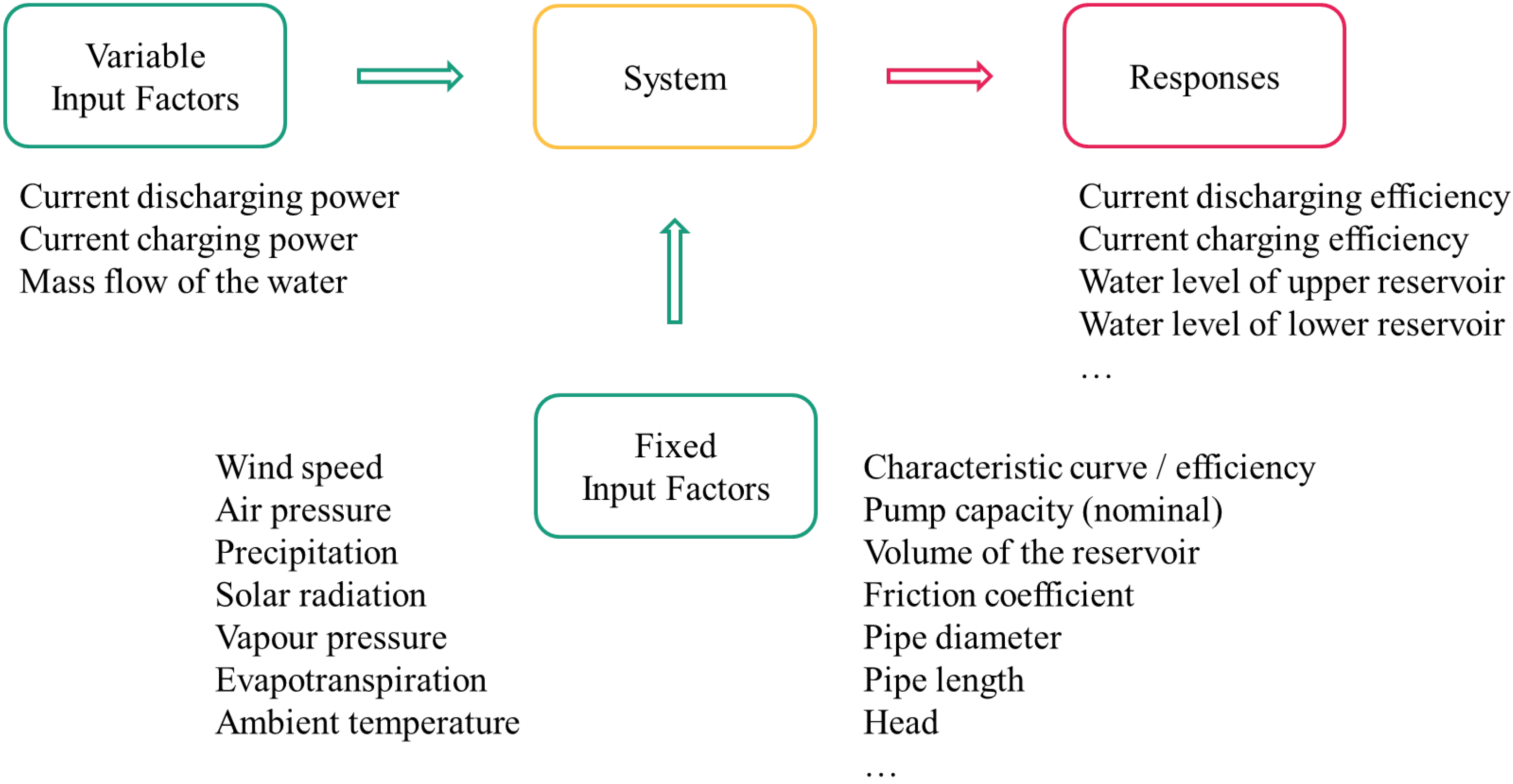
In this section, the application and the results of the parameter diagram method are presented. As described in Section 2.1, there are different parameters and factors influencing the system, and at the same time, there are different system responses. Subsequently, all parameters and factors potentially related to the PHES system are divided into two categories—variable and fixed input factors. These two categories and corresponding factors can be found in Figure 3. Only the responses and not the error states are considered as system outputs since the simulation runs deliver only desired system outputs.
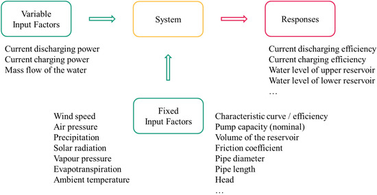
Figure 3.
Parameter diagram with a selection of factors and responses. Own representation based on [14].
Figure 3 gives an overview of the parameters, factors, and responses for PHES, which are divided into three categories, as mentioned previously. Input factors are the current charging and discharging power and the current mass flow rate, because they can be varied during operation. Among the fixed input factors, the following environmental factors are considered: Wind speed, air pressure, precipitation, solar radiation, vapor pressure, evapotranspiration, and ambient temperature. Furthermore, design-related factors also belong to the fixed input factors, such as the characteristic curve, nominal power, volume of the reservoir, friction coefficient, pipe diameter, and geodetic height. All these input parameters and factors can have a greater or lesser influence on the system and, thus, on the system output. This system output is the current charging and discharging efficiency and the water level in the upper and lower reservoir (later referred to as the state of charge (SOC)).
The efficiency is dependent on the power and this determines the mass flow of the water, as can be derived from characteristic curves. So there is a direct relationship between the two input factors and also between input and output in each case. These two input factors can be changed during operation, which is why they are categorized here as variable input factors. Only the power is part of the experimental design due to the correlation between the current power and mass flow. The SOC, which is the amount of water in the reservoir, can be affected by wind speed, air pressure, precipitation, solar radiation, and ambient temperature. Thus, in contrast to the air pressure, these factors are included in the experimental design. The reason for neglecting air pressure in the consideration is its little capacity for variability in just small ranges of values and, thus, is assumed to be constant. However, evaporation is also an influencing factor, among others, it is simultaneously influenced by wind speed and ambient temperature, and is, therefore, not included as a separate factor in the experimental plan.
In Section 2.1, the system input is described as factors that are part of the experimental plan and as parameters that are not included in the plan and should be kept constant during the simulation. The variable input factors in Figure 3 and the fixed input factors that vary over time, for example, wind speed, are taken into account within the plan. The other fixed input factors are design parameters, such as pipe diameter, and are not included in the experimental plan since they are neither adjustable nor changeable during storage operation. For the factor’s value ranges, see Section 3.2.2.
3.2. Step 2: Dynamic Simulation
The dynamic PHES model used for the presented tool chain and to generate relevant data sets was created via the modeling language Modelica using the user interface Dymola (Dynamic Modeling Laboratory) in version 2021x (64-bit) [27]. The model is based on the commercially available component library Hydro Power Library from Modelon, which provides a framework for modeling and simulation of hydropower plant operation [28].
The overall model of the PHES generally consists of the following main components: Pump, turbine, upper and lower reservoir, penstocks, motor, generator, and PID controller. The structure and functionality of these components are described in [29]. Additionally, to investigate the influence of atmospheric conditions on the performance of the PHES plant, the effect of evaporation and precipitation in the upper reservoir according to [30] was implemented in the model. The following section is focusing on design parameters and implemented control strategy relevant to the tool chain.
3.2.1. Description of the PHES Model
The PHES model describes a closed-loop plant with ternary machine sets (separate motor-generator, turbine, and pump). The most important parameters are listed in Table 2. The parameterization of the plant is based on the existing plant Mapragg in Switzerland. Further data, such as the nominal flow rates of the pumps and turbines, as well as the dimensioning of the penstocks, can be found in [31].
Table 2.
Design parameters of the PHES.
Since the case study carried out in this work is only considering the charging process of the PHES, it is described in more detail in the following. The electrical power consumption of the pumps is kept constant over the entire charging process by a variable speed drive. The minimum partial load for each pump is set to 0.3 of its nominal load. The number of pumps operating simultaneously is depending on the given set point value of the charging power of the overall system. In addition, it is specified that the pumps in operation always transport the same amount of water and, thus, consume the same power.
For a time-efficient analysis of parameter variations on the performance of the PHES plant, important key figures of the overall system are calculated automatically in the model. The most important evaluation parameter for the charging process is the charging efficiency . It is determined by the energy supplied to the upper reservoir (potential energy) and the energy consumed in the motor-driven pumps during the entire charging process .
3.2.2. Design of Experiments for PHES
In the previous screening, the influencing parameters and factors were determined. For each individual factor included in the experimental plan, a minimum and maximum value have to be defined (cf. Table 3). The experimental plan is designed with the software optiSLang (2021 R1). It is necessary to insert the factors and their value limits into the plan and then select a suitable sampling method (here, Advanced Latin Hyper Cube). OptiSLang is linked to the modeling and simulation environment Dymola to run as many simulations as specified in the experimental plan.
Table 3.
Factors with corresponding limits used in the experimental design.
In the investigated simulation model, three pumps are modeled, which leads to the following ranges for the storage power: The relative charging power when operating one pump is up to 33.4% when operating two pumps between 33.4% and 66.8%, and when operating three pumps between 66.8% and 100% of the installed power. The initial state of charge () can vary between 0% and 99% of the maximum storage capacity. The difference between and the maximum storage capacity (100%) is and can vary between 1% and 100%. The ambient temperature is set within the limits of 253.15 K and 313.15 K, the relative humidity between 0% and 100%, and the net radiation between 0 W m and 1000 W m. The limits for the precipitation are 0 m s and 1.2222 10 m s and for the wind speed at 2 m height between 0 m s and 14 m s.
With these factors, their value limits, and the sampling method ALHC, the simulation described in Section 3.2.1 is performed. By using the ALHC, the correlation errors are minimized by using stochastic evolution strategies, and the factor’s distribution is uniformly generated. As explained in Section 2.3, a sample size of at least 600 samples is deemed sufficient for deriving the linear surrogate model from the simulation model. As around half of the simulation runs failed in smaller data acquisition tests, due to the imposed constraints in the simulation model, it was decided to begin the simulation with 1500 factor-samples, resulting in around 700 usable instances of data for future use.
Table 4 shows an excerpt of the results calculated under consideration of the limits in Table 3. In addition to the factors, the system response, the efficiency , is also shown in the table.
Table 4.
Design of Experiments—results.
With the help of the DoE, a uniformly distributed analysis of the technical properties and environmental influences is made possible. These simulation results are subsequently used in the regression analysis in the following section to investigate the influences of the input factors on the efficiency. A transpose of this data is used as the data matrix X for the OLS-regression algorithm and Equation (3). Prior to further analysis, each column is z-standardized to .
3.3. Step 3: Regression Analysis
The overarching goal of the presented tool chain is to provide a flexible approach to improving the representation of energy storage systems in energy system models. As already stated, the commonly used constant models (level 0) for storage systems can be too simplistic to predict efficiency variations arising from generally nonlinear energy storage cycles accurately.
In this section, around 700 predictions by the previously introduced level 3 simulation model for the charging state of a PHES system were used to inform a piecewise linear regression model. This section summarizes the regression analysis results, showing that the constructed model is highly consistent with the foundational simulation model (mean absolute error of 0.5 percentage points between the linear and nonlinear prediction, and an larger than for the simulation data).
3.3.1. Data Analysis
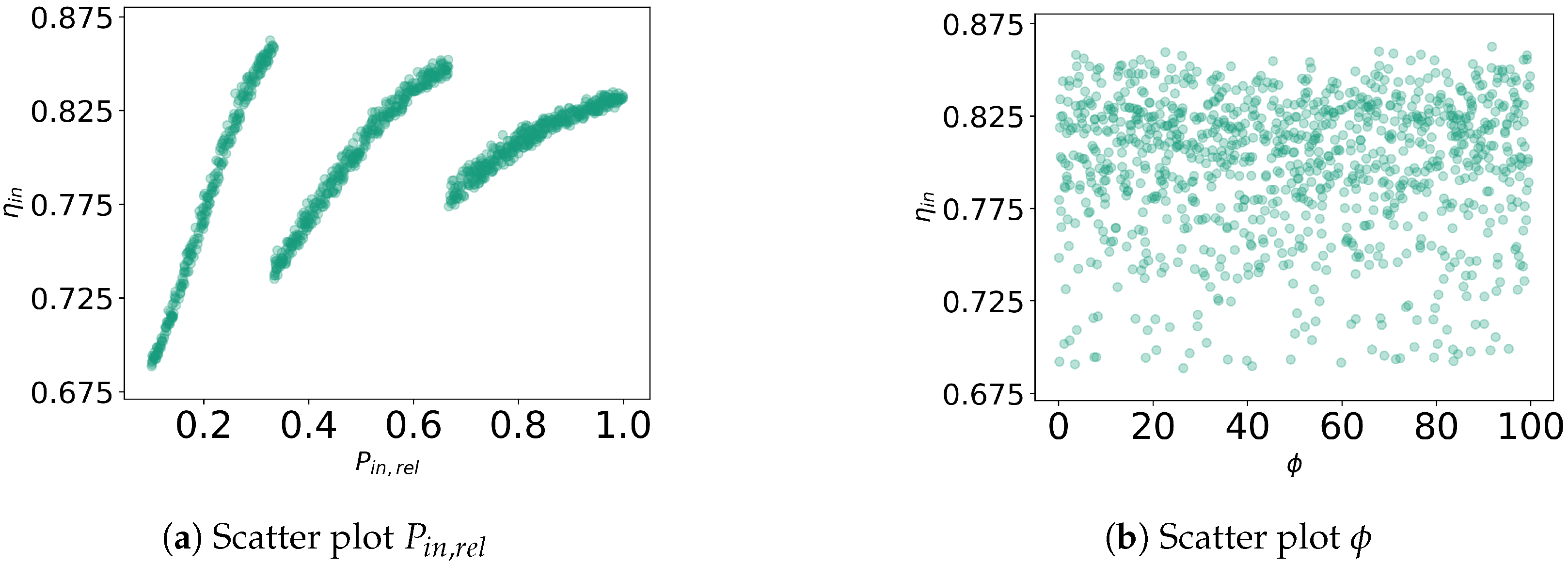
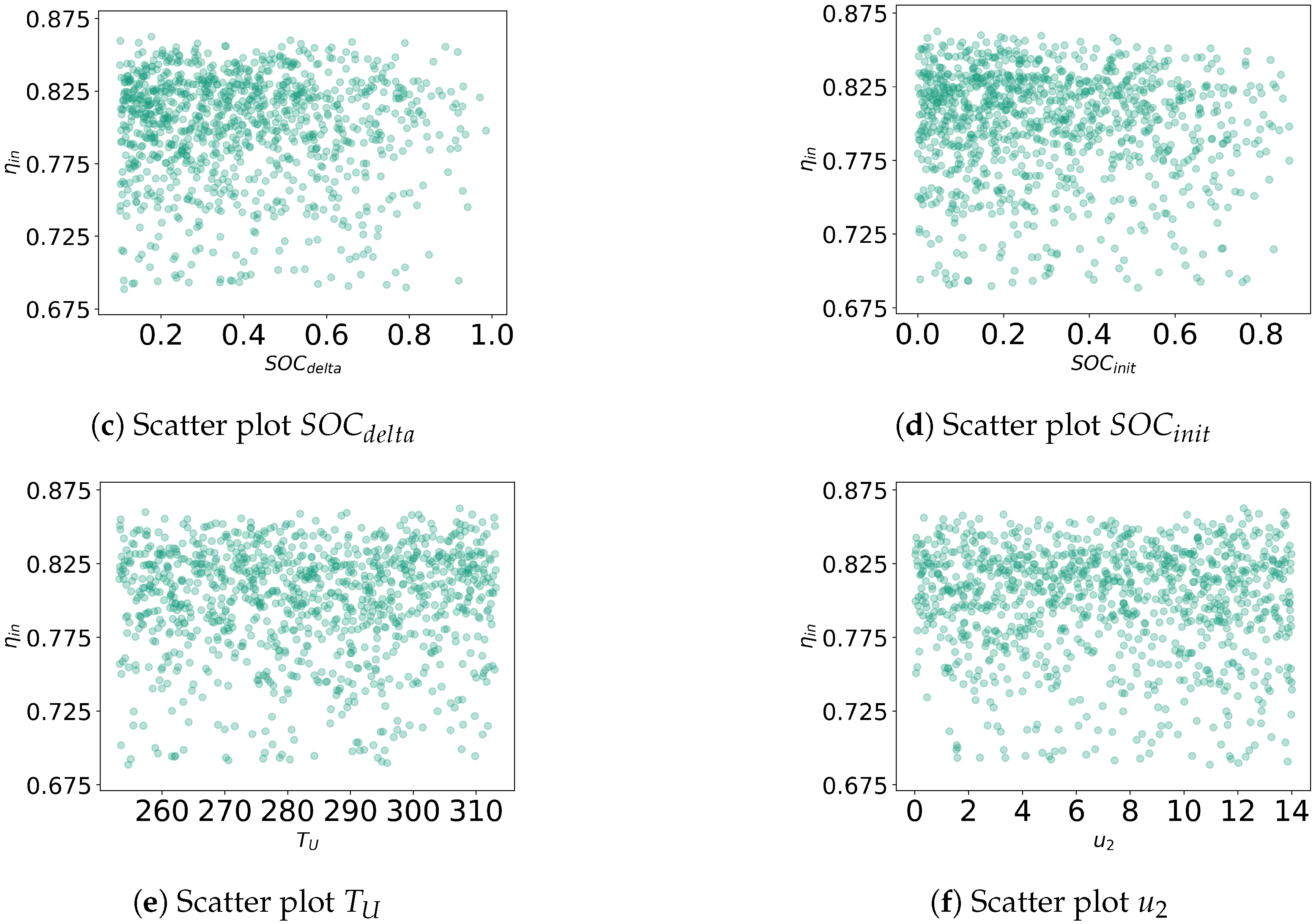
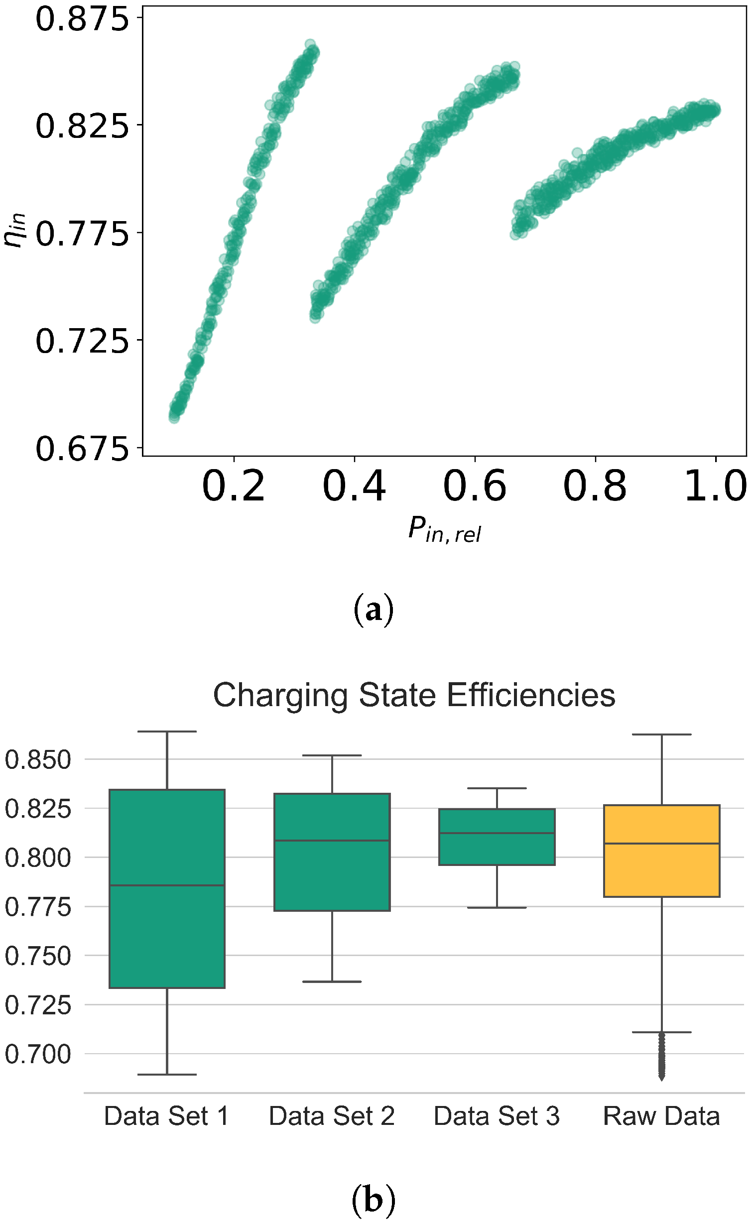
At the beginning of this regression analysis, the 700 simulation data samples are preprocessed for IQR outliers; correlation coefficients are computed and analyzed for selecting model input factors x. For the charging state, the scatter plots of the screened factors and the charging state efficiency suggested partitioning the (raw) data set into three sub-data sets according to their value of :
- Sub-data set 1:
- Sub-data set 2:
- Sub-data set 3: .
This partitioning is founded on the observed piecewise-linear relationship between and (Figure 4a) and no discernible relationship between any other factor and (Appendix A.1).

Figure 4.
(a) Scatter plot for raw data showing the relation between and charging state efficiency , and (b) box plot showing the IQRs (boxes and lines) and classified outliers (black diamonds) for on the partitioned data sets (green) and the raw data (orange).
Observing the data, partitioning the raw data set (all 700 samples) promises to increase the accuracy of predicting by using a piecewise linear model instead of a standard linear regression, based on the scatter plots. To follow up on this hypothesis, a comparative (IQR-)outlier analysis (Figure 4b) reveals that all samples with are classified as outliers, as such efficiency values were rather extreme on a global scale (Figure 4b, black diamonds in the orange box plot). In contrast, the outlier analysis of each sub-data set showed that no sample contains atypical values, which is also suggested by the scatter plots. Hence, the suggested partitioning of the data accounts for the “local variance” of and therefore keeps the typical information on the modeled charging state for further analysis steps.
3.3.2. Correlation Analysis
To further elaborate whether a piecewise-linear model is more suitable for simplifying the level 3 model, a correlation analysis followed, further arguing for the data partitioning and the importance of in a (piecewise) linear model. Table 5a–d show the correlation matrices for all 4 defined (sub-)data sets.
Table 5.
Correlation matrices for the three partitioned data sets and the raw data set, based on the highest absolute Pearson correlation coefficients of a (screened) variable x with in data set .
In each matrix, those three input factors x with the largest absolute correlation coefficient with the state efficiency are listed, as these are the most suitable candidates for the design of a linear model; all full correlation matrices are listed in Appendix A.2. For each data set, significant correlations with only show for . The environmental input factors such as precipitation , humidity , and wind velocity show no significant correlation with .
In contrast to other publications, such as [32,33,34], the initial state of charge can also be neglected. This is a direct result of the way the level 3 model of the PHES is set up (cf. Section 3.2.1). By choosing a control strategy for the PHES that keeps the power constant over the whole charging process, the influence of the state of charge on the required charging power is mitigated by the controller and is instead included indirectly in the charging efficiency.
Hence, only is to be selected for the (piecewise) linear model. Underlining the observations in the scatter plots, the correlation analysis on the three sub-data sets indicates a near-perfect linear relationship between and (, Table 5a–c), whereas for the raw data, just weakly correlated with (, Table 5d). All gained insights, hence, argue for the use of three sub-data sets and for simplifying the previously modeled PHES charging state as follows:
3.3.3. Assumption Analysis
After defining and scaling all three training and test data sets, model coefficients were calculated using OLS for each training data set. By using the test data sets, predictions, and residuals were then computed to check for the classical assumptions of linear regression, revealing heteroscedasticity [25] (pp. 94–96) in all three cases (see Appendix A.3). As all further assumptions were met, the heteroscedasticity-robust White variance estimator [35] is chosen for the following t-tests.
3.3.4. Coefficient Analysis
Using heteroscedasticity-robust White variance estimates for all three data sets, t-Statistics [24] (pp. 117–119) were computed for the standard t-test for each estimate (Table 6a). The 99% confidence intervals for each model coefficient are then computed using the estimation errors , showing that the coefficients (computed with each training data set) are suitable for a flexible use of a piecewise linear model for describing the discussed PHES charging state. Unsurprisingly, the connoted p-values for all t-tests are close to machine precision.
Table 6.
Coefficient Estimation errors , and Prediction Errors for the three sub-data sets | | . These errors are used for the 99% Coefficient Confidence Prediction Intervals.
Following up the coefficient analysis, the computation of prediction errors , shows that the constructed piecewise linear model with coefficients consistently estimates the efficiency values of the level 3 model correctly up to an error slightly larger than with a certainty of 99%. It can therefore be expected that the piecewise linear model will predict similar values to the level 3 model, when using the regression coefficients presented in Table 6a and when inputting .
3.3.5. Performance Analysis
A key motivation for this research was to improve the representation of the PHES in energy system models, as constant models fail to account for changes in efficiency levels due to changes in the input factors. Computing widely-known performance metrics show that a constant efficiency prediction performed significantly worse in matching the level 3 model when compared to a piecewise linear prediction.
Table 7 summarises the inability of the constant model to accurately represent the variance of with changing input values (). In contrast, the piecewise linear model (8) captured nearly all variance of in all cases (), illustrating the congruence between the level 3 and level 1 models in predicting . No further inputs are deemed necessary.
Table 7.
Comparing Regression Model and Constant Model Performances on the Test Data (75–76 data points) for each sub-data set ||. For the constant model evaluation, the mean efficiency value of all three training data sets and the metrics for all three test data sets were computed.
To sum it up, the performed regression analysis exemplified the potential of the suggested tool chain, and showed that careful data analysis and a slight increase in complexity can lead to a high increase in the prediction performance of a linear model over a constant representation of an energy storage unit in an energy system model.
3.4. Step 4: Refining Optimization Model
As the previous sections have shown, to depict the charging process of a PHES more accurately, it is necessary to model the dependence of the charging efficiency on the current charging power. The new model should therefore adapt Equation (6).
It is not possible to include this dependency directly in Equation (6), since it would lead to a nonlinear constraint (most of the national and transnational energy system models are linear or mixed-integer linear models). Instead, the charged energy in time step t can be calculated separately and subsequently be added to the state of charge of the previous time step.
The relation between the net charged power and the charging power can be calculated from the simulation data by multiplying each charging power with its corresponding charging efficiency. This leads to a nonlinear function for , which in turn can be linearized using SOS2-variables .
Figure 4 shows the obtained data for and the corresponding . This data is used to calculate . To determine and , discontinuities in the data were identified. This is done by approximating the gradients and selecting the points with the highest absolute values. Additionally, adding the value at the minimum and maximum charging power allowed for covering the whole interval. Table 8 shows a summary of the breakpoint values for the analyzed charging process of the PHES.
Table 8.
Breakpoint values for the analyzed charging process of the PHES.
4. Discussion
In this paper, we developed a tool chain to investigate the modeling and parametrization of simplified storage models based on the detailed simulation of a physical model. The tool chain was carried out using the example of a pumped hydroelectric storage model. It was shown that the tool chain is well suited to identify the relevant influencing factors which have to be modeled in simplified models to still accurately represent the behavior of the storage model in the desired use case. In addition the tool chain yields the necessary parameterization of the simplified model, which is consistent with the detailed physical model of the real world system.
The steps of the developed tool chain are generic and, as such, can be used to analyze other (storage) technologies and desired levels of simplification. The identified parameters for the experimental plan of the PHES investigation can be used for other mechanical storage technologies with only small adjustments. Further influencing factors can be analyzed by including them in the experimental plan. For example, it is possible to investigate the influence of aging, by adding a state of health parameter. The representation of the resulting correlation in the level 1 MILP model is the subject of ongoing research though.
For all results of the tool chain, including the ones of the case study in this paper, the level 3 model has a great influence on the results. It is, therefore, necessary to be very careful when designing the level 3 model and to include all relevant physical dependencies in enough detail. In addition the chosen control strategy for the technology can also greatly influence the results of the tool chain as shown in Section 3.3.2. An alternative to using level 3 simulation models as data input into the tool chain is to use measured data, if it is available for the whole range of the experimental plan. In this case all relevant physical parameters should be included in the data, as well as the applied control strategy.
For the simplified PHES model derived in this paper, it was shown that the piecewise linear regression model reproduces the variance in the simulation data quite accurately (). Moreover, the values of the level 3 model can be predicted correctly to within 6 percentage points of expected prediction error. With a range of about 45 percentage points in storage efficiency, this is a relevant improvement over a constant PHES model, which showed an average error of 19% in the data used.
In the future, in the context of the energy industry and further, we expect the application of statistics and AI to increase generally. These powerful tools complement areas of supply security, efficiency, and technological advancement. The aim of future work is to quantify the impact the derived simplifications of the level 1 model have on the results and the performance of the large-scale energy system models. To achieve this, besides the analysis of the charging process shown in this paper, we also investigated the storage and discharging process of the same pumped hydro electric storage system. In addition we are going to use the tool chain to analyze different configurations of PHES systems as well as compressed air energy storage systems.
Author Contributions
Conceptualization, E.S., K.W., T.S., A.M. and M.H.; methodology, K.W., T.S., E.S. and M.H.; software, K.W., T.S., E.S. and M.H.; validation, T.S. and E.S.; formal analysis, T.S.; investigation, K.W., T.S., E.S., M.H. and S.P.; resources, K.W., T.S., E.S., M.H. and S.P.; data curation, K.W. and T.S.; writing—original draft preparation, K.W., T.S., E.S. and M.H.; writing—review and editing, K.W., E.S., S.P. and A.M.; visualization, K.W., T.S. and M.H.; supervision, A.M.; project administration, A.M., E.S. and K.W.; funding acquisition, A.M. All authors have read and agreed to the published version of the manuscript.
Funding
The project “Sesame Seed” was funded by the Federal Ministry of Economics and Climate Protection in Germany (BMWK) FKZ 03EI1021 within the framework of the joint project “Open Sesame-Modelling of energy storages for simulation/optimization of energy systems”.
Data Availability Statement
Not applicable.
Acknowledgments
Thanks goes to Christian Doetsch from Fraunhofer Institute for Environmental, Safety, and Energy Technology UMSICHT for initiating and facilitating the Open Sesame project and for the initial idea for classifying energy system models into different levels of detail.
Conflicts of Interest
The authors declare no conflict of interest. The funders had no role in the design of the study; in the collection, analyses, or interpretation of data; in the writing of the manuscript, or in the decision to publish the results.
Abbreviations
The following abbreviations are used in this manuscript:
| I | Precipitation around the upper reservoir of a PHES system |
| IQR | Interquartile Range |
| OLS | Ordinary Least Squares |
| Net charged power in timestep t | |
| Net charged power at breakpoint n | |
| Net discharged power in timestep t | |
| Electrical charging power at breakpoint n | |
| Maximum electrical charging power | |
| Relative electrical charging power | |
| Electrical charging power in timestep t | |
| Electrical discharging power in timestep t | |
| Maximum electrical discharging power | |
| Electrical discharging power at breakpoint n | |
| PHES | Pumped hydroelectric energy storage |
| Coefficient of Determination | |
| Irradiance | |
| Difference between states of charge at timesteps t + 1 and t | |
| State of charge at the start of a simulation run | |
| Maximum state of charge | |
| State of charge in timestep t | |
| Ambient temperature of the upper reservoir of a PHES system | |
| Wind Speed around the upper reservoir of a PHES system | |
| Duration of one timestep | |
| Constant charging efficiency | |
| Constant discharging efficiency | |
| SOS2 variable | |
| Humidity around the upper reservoir of a PHES system |
Appendix A. Auxiliary Results for the Regression Analysis Example
Appendix A.1. Scatter Plots for Individual Influencing Parameters against Charging State Efficiency
The charging state simulation data set was subdivided based on the visible piecewise linear relationship between the relative input electric power and the charging state efficiency , as well as no clarly visible relationships between all further variables and . The following figures provide an extensive list of all scatter plots observed before deciding for the data partitioning described in Section 3.3.
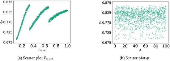
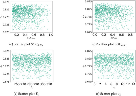
Figure A1.
Scatter plots for raw data showing different features and charging state efficiency .
Figure A1.
Scatter plots for raw data showing different features and charging state efficiency .
Appendix A.2. Pearson Correlation Coefficient Matrices
Based on the Pearson correlation coefficient between an input variable and the efficiency y, a subset of all was selected for the linear regression model, if the absolute value of a coefficient was larger than 0.4. In the example given in Section 3.3, four data sets were analyzed simultaneously (the three constructed sub-data sets and the raw data), and the Correlation Coefficient Submatrices for the three parameters with the largest absolute coefficient were shown. The full correlation matrices are given below.
Table A1.
Full Pearson Correlation Coefficient Matrices.
Table A1.
Full Pearson Correlation Coefficient Matrices.
| (a) . | ||||||||
| I | ||||||||
| −0.015 | 1 | |||||||
| 0.049 | 0.007 | 1 | ||||||
| 0.038 | −0.002 | 0.023 | 1 | |||||
| −0.001 | 0.03 | −0.002 | −0.524 | 1 | ||||
| −0.033 | −0.012 | 0.01 | −0.029 | 0.002 | 1 | |||
| I | −0.019 | 0.026 | 0.015 | −0.018 | 0.007 | 0.024 | 1 | |
| 0.012 | −0.02 | 0.018 | 0.03 | 0.001 | 0.048 | 0.016 | 1 | |
| 0.994 | −0.018 | 0.051 | 0.046 | −0.061 | −0.037 | −0.019 | 0.01 | |
| (b) . | ||||||||
| I | ||||||||
| 0.003 | 1 | |||||||
| −0.023 | 0.015 | 1 | ||||||
| 0.006 | 0.019 | −0.009 | 1 | |||||
| 0.034 | 0.04 | 0.009 | −0.514 | 1 | ||||
| −0.011 | 0.016 | 0.026 | 0.015 | −0.005 | 1 | |||
| I | 0.023 | 0.005 | 0 | −0.028 | 0.007 | −-0.064 | 1 | |
| −0.029 | 0.004 | 0.015 | 0 | −0.041 | 0.007 | −0.026 | 1 | |
| 0.984 | −0.03 | −0.022 | 0.016 | −0.072 | −0.009 | 0.028 | −0.024 | |
| (c) . | ||||||||
| I | ||||||||
| −0.034 | 1 | |||||||
| 0.004 | 0.023 | 1 | ||||||
| −0.016 | 0.02 | 0.021 | 1 | |||||
| −0.052 | 0.009 | 0.024 | −0.512 | 1 | ||||
| −0.021 | 0.01 | 0.036 | 0.024 | −0.04 | 1 | |||
| I | −0.019 | 0.003 | 0.013 | 0.016 | 0.037 | −0.028 | 1 | |
| 0.04 | 0.013 | 0.002 | −0.032 | 0.042 | −0.06 | −0.013 | 1 | |
| 0.968 | −0.044 | 0 | 0.019 | −0.231 | −0.009 | −0.027 | 0.025 | |
| (d) Raw charging state data. | ||||||||
| I | ||||||||
| −0.029 | 1 | |||||||
| −0.018 | −0.042 | 1 | ||||||
| −0.006 | −0.024 | −0.014 | 1 | |||||
| −0.004 | −0.028 | 0.013 | −0.492 | 1 | ||||
| −0.018 | −0.029 | 0.01 | −0.013 | 0.003 | 1 | |||
| I | −0.015 | −0.062 | 0.026 | −0.029 | 0.048 | −0.055 | 1 | |
| 0.02 | 0.002 | 0.017 | 0.025 | 0.009 | −0.042 | −0.021 | 1 | |
| 0.492 | −0.007 | −0.047 | −0.023 | −0.066 | −0.005 | 0.026 | −0.028 | |
Appendix A.3. Qualitative Analysis of the Coefficient Estimates
The adaptations of the statistical tests/quantitative analysis of the regression parameters resulted from the insights of the qualitative analysis of the OLS estimator for the BLUE property in the three sub-data sets. With this section, all results of the qualitative analysis are summarised to make transparent why only adaptations for heteroscedasticity were neccessary.
- Linearity
The piecewise regression model is, due to its definition as a matrix-vector product, linear in its model parameters . The assumption holds by design.
- Zero Expected Error
For OLS to be the Best Linear Unbiased Estimator, it needs to be shown that the model error u is expected to be 0. As this population property for the linear model cannot be computed (the population/input variable space is infinitely large), the “sample mean estimator” is used to computing the expected error of the unknown quantity u. This means that for checking this assumption, the mean value of all training data residuals was computed. As these sample means were all close to machine precision (), it was concluded that this BLUE assumption is satisfied.
- Only Exogenous Influencing Parameters
Exogeneous Influencing Parameters show “no correlation” with the regression error term u. Again, as the exact form of the regression error is unknown; this condition is tested by computing the Pearson correlation coefficients of each selected influencing parameter with the residual of the computed OLS/piecewise linear model. Again, all correlation coefficients were close to machine precision ( to ), and therefore it could be concluded that the variable is exogenous, and this condition to hold.
- No Multicolinearity
As only a single variable was selected for the piecewise linear regression model, a perfect linear correlation between two different parameters is not possible. In other terms, no parameter can be described as a linear combination of all other parameters as there is no other parameter. Hence, there is no multicolinearity in the piecewise model.
- No Heteroscedasticity
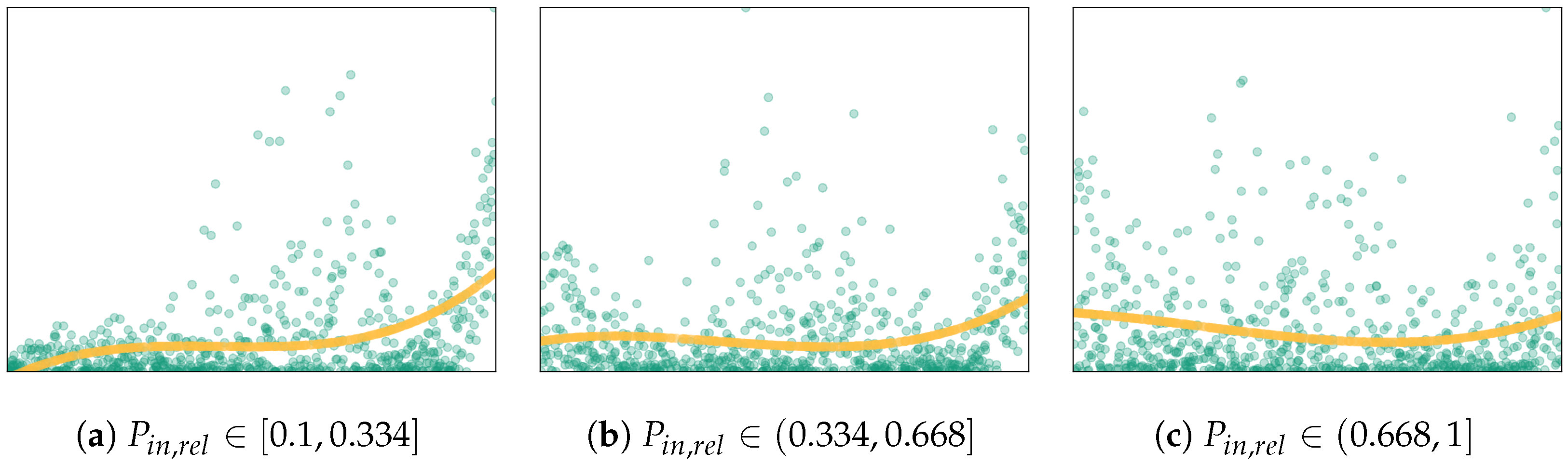
As already sketched in the main body of this paper, all three residuals for data sets were tested for heteroscedasticity with the Breusch–Pagan test. The basis of this test is to construct a regression model for the squared residuals using the input variable of the regression model with which the residuals were calculated. The squared residuals are used as an estimator of the variance in the error term of the tested regression model (in this case, the piecewise linear regression model). For the given example, the “Breusch–Pagan test model” reads as following:
The coefficients are computed by applying the OLS estimator to the transformed data matrices where is the data vector obtained by elementwise squaring or cubing the of the values in . Having computed the coefficients , linearity tests on each data set were used to check whether any coefficient significantly differs from 0. If so, the respective linear submodel would produce heteroscedastic residuals.
The results of the Breusch–Pagan model showed that all three linear submodels significantly differ from a constant model, and, therefore, signal that the regression error of the piecewise linear model is heteroscedastic. Based on the computed coefficients , an orange prediction/regression line was plotted in Figure A2.
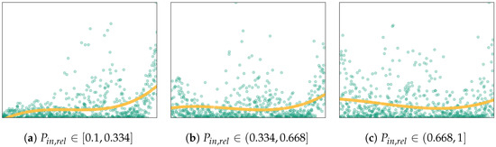
Figure A2.
Scatterplots (blue) of squared OLS residuals (y-axis) against feature (x-axis) for the charging state data sets. The Breusch–Pagan test suggests heteroscedasticity for all three data sets (as the orange prediction lines are not constant).
Figure A2.
Scatterplots (blue) of squared OLS residuals (y-axis) against feature (x-axis) for the charging state data sets. The Breusch–Pagan test suggests heteroscedasticity for all three data sets (as the orange prediction lines are not constant).
- No Autocorrelation
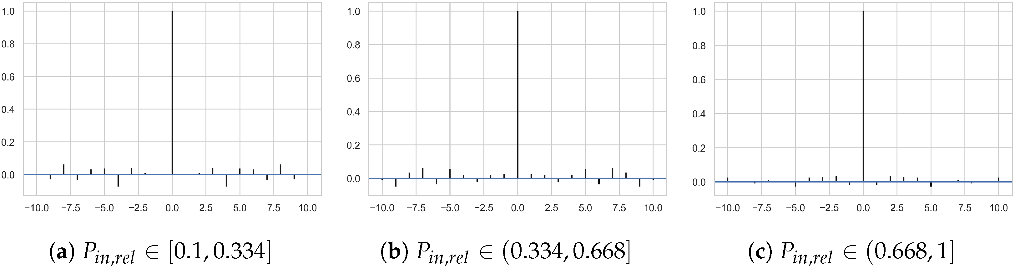
Autocorrelating regression errors are described by the potential to predict a single error accurately based on previously computed/other errors . Such errors do typically appear in time-series data which is structurally different from the cross-sectional data used in the outlined tool chain. Still, there is the need to check for autocorrelation, for example, by using autocorrelation plots and the Durbin–Watson tests.
The shown autocorrelation plot in Figure A3 suggests the absence of autocorrelation in each data set. Similar results also show for the Durbin–Watson test. This test computes the Durbin–Watson statistic
for the residuals of each data set. If the resultant value is “close to 2” (for this tool chain: ranging from 1.9 to 2.1), the test would suggest that autocorrelation is absent from the regression error . The statistics for the three relevant data sets ranged from 1.94 to 2.04, which further suggests the absence of autocorrelation in the regression error of the piecewise linear model.
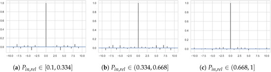
Figure A3.
Autocorrelation plots for all three residuals obtained from the linear submodels for data sets . The appearance of any bars but one at being visibly larger than 0.1 suggests autocorrelation of the respective residuals.
Figure A3.
Autocorrelation plots for all three residuals obtained from the linear submodels for data sets . The appearance of any bars but one at being visibly larger than 0.1 suggests autocorrelation of the respective residuals.
References
- Washington Post Staff. The Glasgow climate pact, annotated. Washington Post, 13 November 2021. [Google Scholar]
- IEA-ETSAP. TIMES Version 4.6.1. 2022. Available online: https://zenodo.org/record/6412545#.Y9jNe63MJPY (accessed on 19 January 2022).
- DlR Institut für Vernetzte Energiesysteme. Energiesystemoptimierungsframework REMix. Available online: https://www.dlr.de/ve/desktopdefault.aspx/tabid-16034/25988_read-66795/ (accessed on 19 January 2022).
- Pfenninger, S.; Pickering, B.C. A multi-scale energy systems modelling framework. J. Open Source Softw. 2018, 3, 825. [Google Scholar] [CrossRef]
- Aghahosseini, A.; Bogdanov, D.; Ghorbani, N.; Breyer, C. Analysis of 100% renewable energy for Iran in 2030: Integrating solar PV, wind energy and storage. Int. J. Environ. Sci. Technol. 2018, 15, 17–36. [Google Scholar] [CrossRef]
- Doetsch, C.; Budt, M.; Wolf, D.; Kanngießer, A. Adiabates Niedertemperatur-Druckluftspeicherkraftwerk zur Unterstützung der Netzintegration von Windenergie; Fraunhofer UMSICHT: Oberhausen, Germany, 2012. [Google Scholar]
- Buffa, F.; Kemble, S.; Manfrida, G.; Milazzo, A. Exergy and Exergoeconomic Model of a Ground-Based CAES Plant for Peak-Load Energy Production. Energies 2013, 6, 1050–1067. [Google Scholar] [CrossRef]
- Budt, M. Thermodynamische Analyse Adiabater Druckluftenergiespeicher unter Berücksichtigung Feuchter Luft und Wassereinspritzung Mittels Dynamischer Simulation: Dissertation; Vol. Band 81, UMSICHT-Schriftenreihe; Karl Maria Laufen: Oberhausen, Germany, 2016. [Google Scholar]
- Guo, H.; Xu, Y.; Guo, C.; Zhang, Y.; Hou, H.; Chen, H. Off-design performance of CAES systems with low-temperature thermal storage under optimized operation strategy. J. Energy Storage 2019, 24, 100787. [Google Scholar] [CrossRef]
- Hadam, M. Thermodynamische Analyse Eines Modularen A-CAES Mit Umkehrbar Betreibbaren Turbo- und Kolbenmaschinen. Ph.D. Dissertation, Ruhr-Universität Bochum, Fakultät für Maschinenbau, Bochum, Germany, 2021. [Google Scholar]
- Mazloum, Y.; Sayah, H.; Nemer, M. Comparative Study of Various Constant-Pressure Compressed Air Energy Storage Systems Based on Energy and Exergy Analysis. J. Energy Resour. Technol. 2021, 143, 052001. [Google Scholar] [CrossRef]
- Mucci, S.; Bischi, A.; Briola, S.; Baccioli, A. Small-scale adiabatic compressed air energy storage: Control strategy analysis via dynamic modelling. Energy Convers. Manag. 2021, 243, 114358. [Google Scholar] [CrossRef]
- Schlachtberger, D.P.; Brown, T.; Schramm, S.; Greiner, M. The benefits of cooperation in a highly renewable European electricity network. Energy 2017, 134, 469–481. [Google Scholar] [CrossRef]
- Siebertz, K.; van Bebber, D.; Hochkirchen, T. Statistische Versuchsplanung; Springer: Berlin/Heidelberg, Germany, 2017. [Google Scholar] [CrossRef]
- Rönsch, S. Anlagenbilanzierung in der Energietechnik: Grundlagen, Gleichungen und Modelle für die Ingenieurpraxis; Springer Vieweg: Wiesbaden, Germany, 2015. [Google Scholar] [CrossRef]
- Casey, M. Vorlesung im Fach “Thermische Turbomaschinen”: Turbokompressoren und Ventilatoren (TKV); Vorlesung; Universität Stuttgart: Stuttgart, Germany, 2012. [Google Scholar]
- Traupel, W. Thermische Turbomaschinen, 4th ed.; Klassiker der Technik; Springer: Berlin, Germany, 2001. [Google Scholar]
- Lüdtke, K. Process Centrifugal Compressors: Basics, Function, Operation, Design, Application; Engineering Online Library; Springer: Berlin/Heidelberg, Germany, 2004. [Google Scholar]
- Dynardo GmbH. Methods for Multi-Disciplinary Optimization and Robustness Analysis; Dynardo GmbH: Weimar, Germany, 2017. [Google Scholar]
- Lumley, T.; Diehr, P.; Emerson, S.; Chen, L. The Importance of the Normality Assumption in Large Public Health Data Sets. Annu. Rev. Public Health 2002, 23, 151–169. [Google Scholar] [CrossRef] [PubMed]
- Maxwell, S.E. Sample Size and Multiple Regression Analysis. Psychol. Methods 2000, 5, 434–458. [Google Scholar] [CrossRef] [PubMed]
- Fahrmeir, L.; Heumann, C.; Künstler, R.; Pigeot, I.; Tutz, G. Statistik: Der Weg zur Datenanalyse, 8th ed.; Springer-Lehrbuch; Springer: Berlin/Heidelberg, Germany, 2016. [Google Scholar]
- James, G.; Witten, D.; Hastie, T.; Tibshirani, R. An Introduction to Statistical Learning: With Applications in R; Corrected at 8th Printing 2017 ed.; Springer Texts in Statistics; Springer: New York, NY, USA, 2017. [Google Scholar]
- Hayashi, F. Econometrics, 1st ed.; Princeton University Press: Princeton, NJ, USA, 2000; pp. 117–119. [Google Scholar]
- Backhaus, K.; Erichson, B.; Plinke, W.; Weiber, R. Multivariate Analysemethoden: Eine Anwendungsorientierte Einführung; Achte, Verbesserte Auflage ed.; Springer eBook Collection Business and Economics; Springer: Berlin/Heidelberg, Germany, 1996. [Google Scholar] [CrossRef]
- Gołebiewski, D.; Barszcz, T.; Skrodzka, W.; Wojnicki, I.; Bielecki, A. A New Approach to Risk Management in the Power Industry Based on Systems Theory. Energies 2022, 15, 9003. [Google Scholar] [CrossRef]
- Dassault Systèmes. DYMOLA Systems Engineering: Multi-Engineering-Modellierung und -Simulation auf Basis von Modelica und FMI; Dassault Systèmes: Velizy-Villacoublay, France, 2021. [Google Scholar]
- Modelon, A.B. Hydro Power Library: Modeling and Simulation of Hydro Power Plants for Performance Analysis, Optimization, and the Development and Verification of Plant Concepts and Control Strategies; Modelon AB: Lund, Sweden, 2018. [Google Scholar]
- Tuszynski, K.; Tuszynski, J.; Slättorp, K. HydroPlant-a Modelica Library for Dynamic Simulation of Hydro Power Plants; The Modelica Association, Modelica Conference: Vienna, Austria, 2006. [Google Scholar]
- Mousavi, N.; Kothapalli, G.; Habibi, D.; Khiadani, M.; Das, C. An improved mathematical model for a pumped hydro storage system considering electrical, mechanical, and hydraulic losses. Appl. Energy 2019, 247, 228–236. [Google Scholar] [CrossRef]
- Zsak, P.; Sigg, R.; Schaffner, C. Bestimmung von Wirkungsgraden bei Pumpspeicherung in Wasserkraftanlagen; Schweizerische Eidgenossenschaft, Bundesamt für Energie BFE Bern: Bern, Switzerland, 2008. [Google Scholar]
- Borghetti, A.; D’Ambrosio, C.; Lodi, A.; Martello, S. An MILP approach for short-term hydro scheduling and unit commitment with head-dependent reservoir. IEEE Trans. Power Syst. 2008, 23, 1115–1124. [Google Scholar] [CrossRef]
- Guisandez, I.; Pérez-Díaz, J.I. Mixed integer linear programming formulations for the hydro production function in a unit-based short-term scheduling problem. Int. J. Electr. Power Energy Syst. 2021, 128, 106747. [Google Scholar] [CrossRef]
- Chen, C.H.; Chen, N.; Luh, P.B. Head dependence of pump-storage-unit model applied to generation scheduling. IEEE Trans. Power Syst. 2016, 32, 2869–2877. [Google Scholar] [CrossRef]
- White, H. A Heteroskedasticity-Consistent Covariance Matrix Estimator and a Direct Test for Heteroskedasticity. Econometrica 1980, 48, 817–838. [Google Scholar] [CrossRef]

Disclaimer/Publisher’s Note: The statements, opinions and data contained in all publications are solely those of the individual author(s) and contributor(s) and not of MDPI and/or the editor(s). MDPI and/or the editor(s) disclaim responsibility for any injury to people or property resulting from any ideas, methods, instructions or products referred to in the content. |
© 2023 by the authors. Licensee MDPI, Basel, Switzerland. This article is an open access article distributed under the terms and conditions of the Creative Commons Attribution (CC BY) license (https://creativecommons.org/licenses/by/4.0/).