

A Novel Stochastic Optimizer Solving Optimal Reactive Power Dispatch Problem Considering Renewable Energy Resources

 ,
,  , ,
, ,  and
and
Abstract
:1. Introduction
- The African Vultures Optimization Algorithm (AVOA) is proposed for the first time to solve a real-world optimization problem such as the ORPD problem.
- In the AVOA, vulture populations are designed with a Levy mutation, which can help to avoid falling into the local minima.
- The suggested AVOA is used to divide the optimization problem into three distinct objective functions (voltage deviation, operating cost, and power loss) as single- and multi-optimization objective functions considering continuous and discrete types of optimization control variables.
- The standard IEEE (30-bus, 57-bus, and 118-bus) testing systems are employed in this research to analyze the impact and demonstrate the consistency of the suggested AVOA algorithm to reach the near-optimal solutions to the self-posed problem and its application scalability on a challenging testing process from the metaheuristic literature.
- The effect of RES insertion on solving the ORPD is analyzed by two methods. The first method is to find the optimal solutions in two steps. The first method is finding the optimal allocation of RES for standard IEEE then determining the optimal solution to the ORPD challenge for the modified IEEE system after inserting the RES in the first step. The second method to find the optimal solution in one step by finding the optimal RES allocation and the rest of the optimal control variables, which means the control variables are increased (problem dimensions increased).
- Finally, IEEE test systems incorporated with the RERs are presented to investigate the dominance of the analyzed AVOA algorithm among other metaheuristic methods for finding the best objective functions solution with fast convergence characteristics.
2. ORPD Problem Formulation
2.1. Objective Functions
2.1.1. Single Objective Functions
Voltage Deviation Minimization
Cost Minimization
Real Power Loss Minimization
2.1.2. Multi-Objective Functions
2.2. System Constraints
2.2.1. Equality Constraints
2.2.2. Inequality Constraints
- -
- Generator Constraints
- -
- Transformer Constraints
- -
- Shunt Capacitor Bank Constraints
- -
- Load Voltage Constraints
- -
- Security Constraints
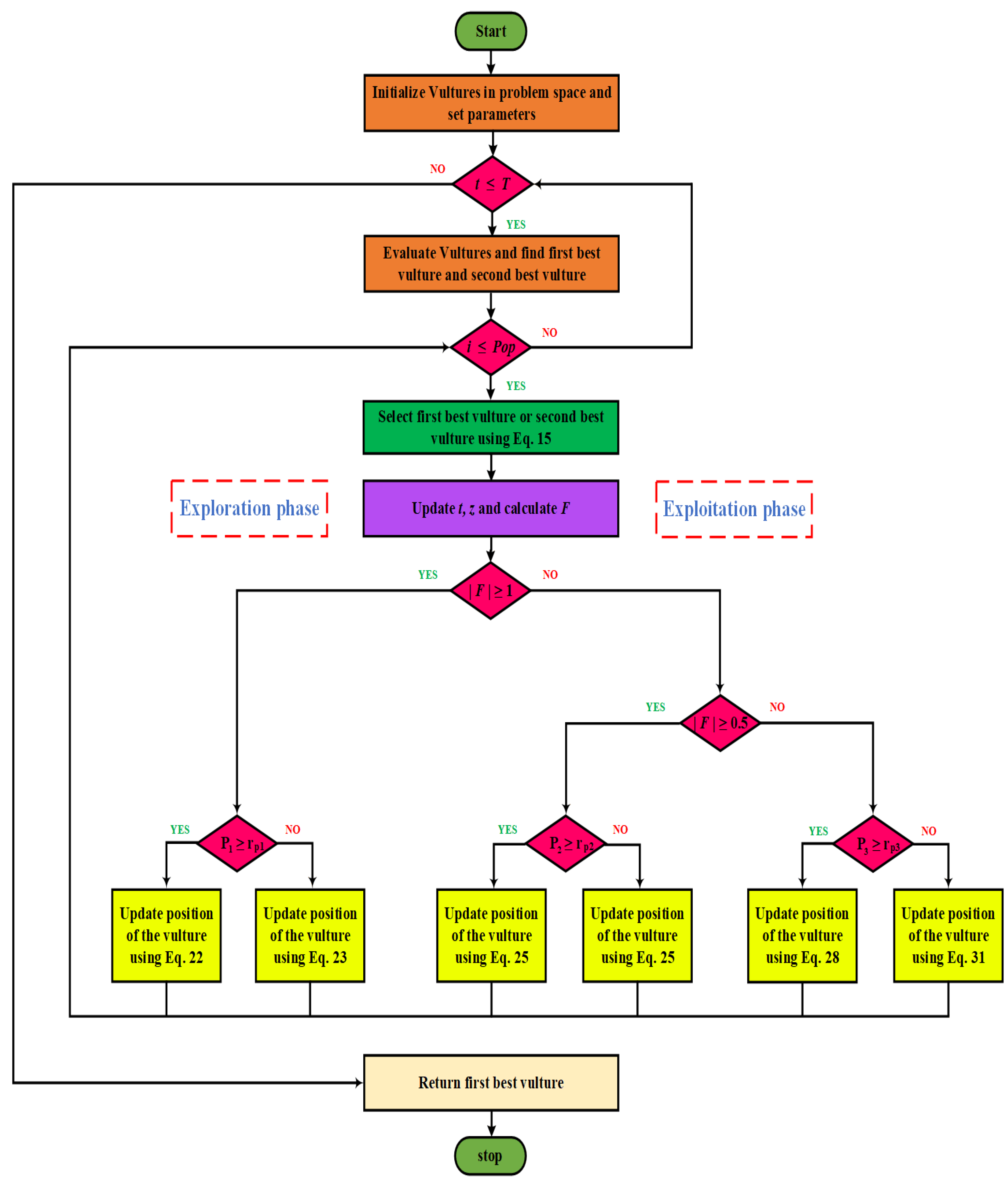
3. African Vultures Optimization Algorithm
- -
- Stage 1: Population Classification
- -
- Stage 2: Vulture Famine Rate
- -
- Stage 3: Reconnaissance Phase
- -
- Stage 4: Utilization Phase (First Stage)
- -
- Stage 5: Utilization Phase (Second Stage)
4. Simulation Results and Discussion
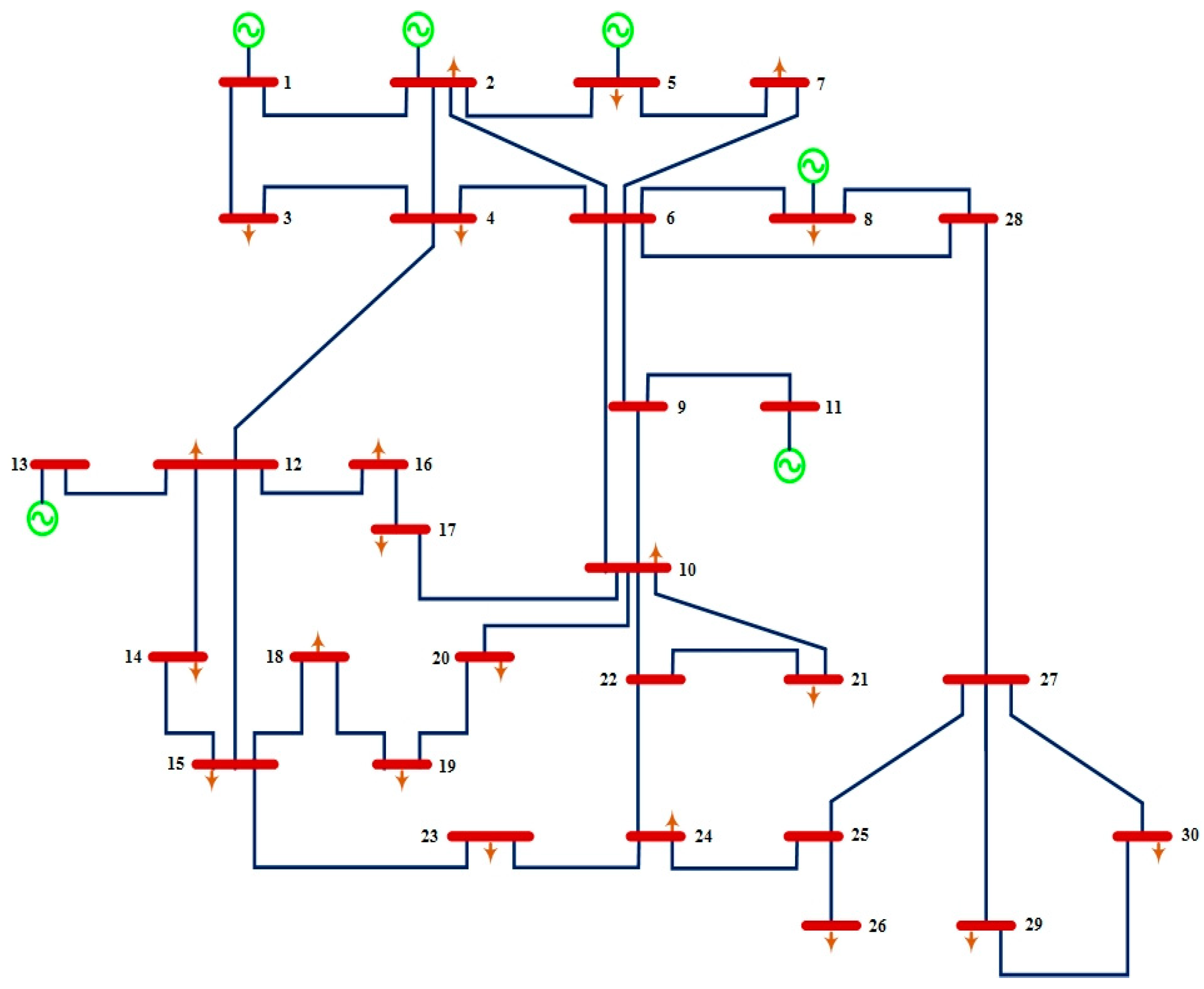
4.1. IEEE 30-Bus Test System
4.1.1. Case 1: Minimization of Voltage-Level Deviation in IEEE 30 Bus
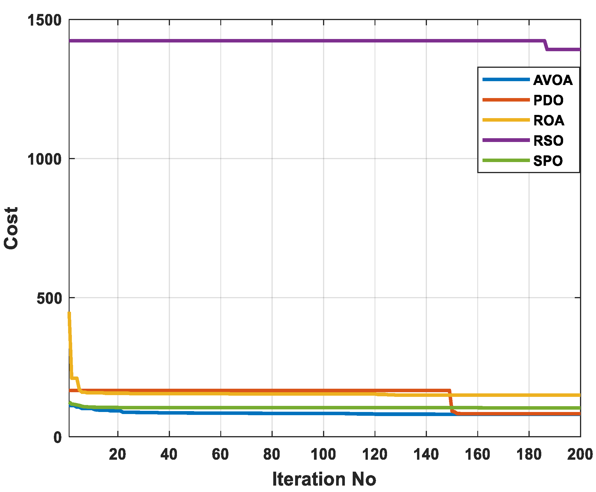
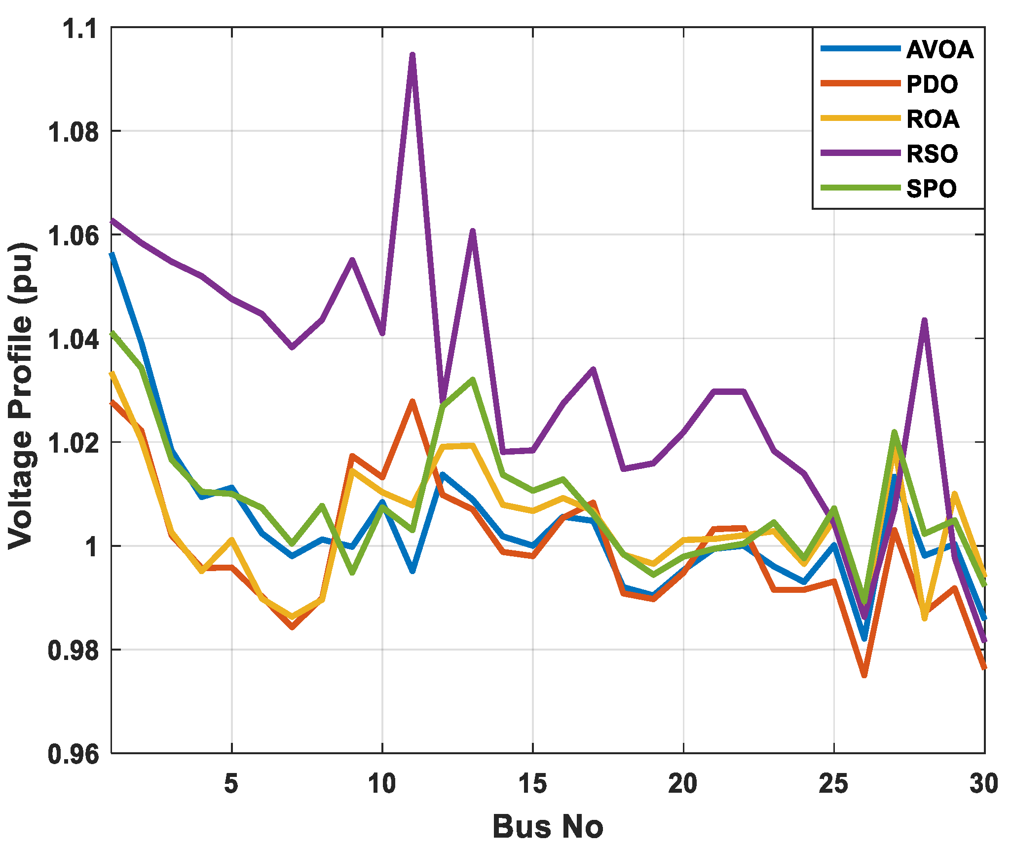
4.1.2. Case 2: Minimization of Operational Cost in IEEE 30 Bus
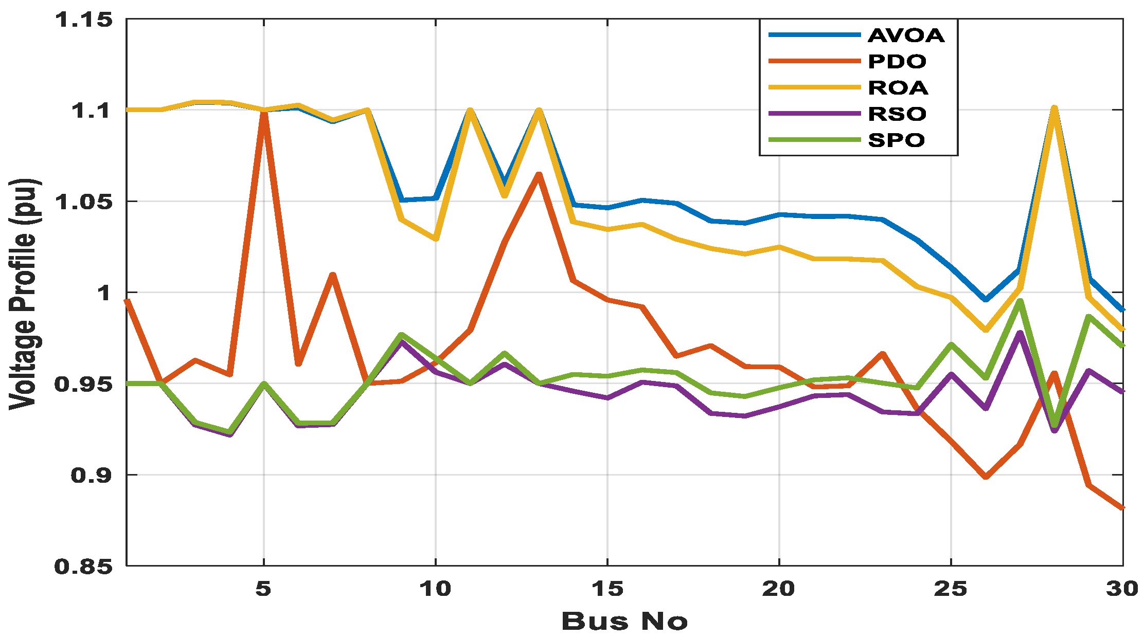
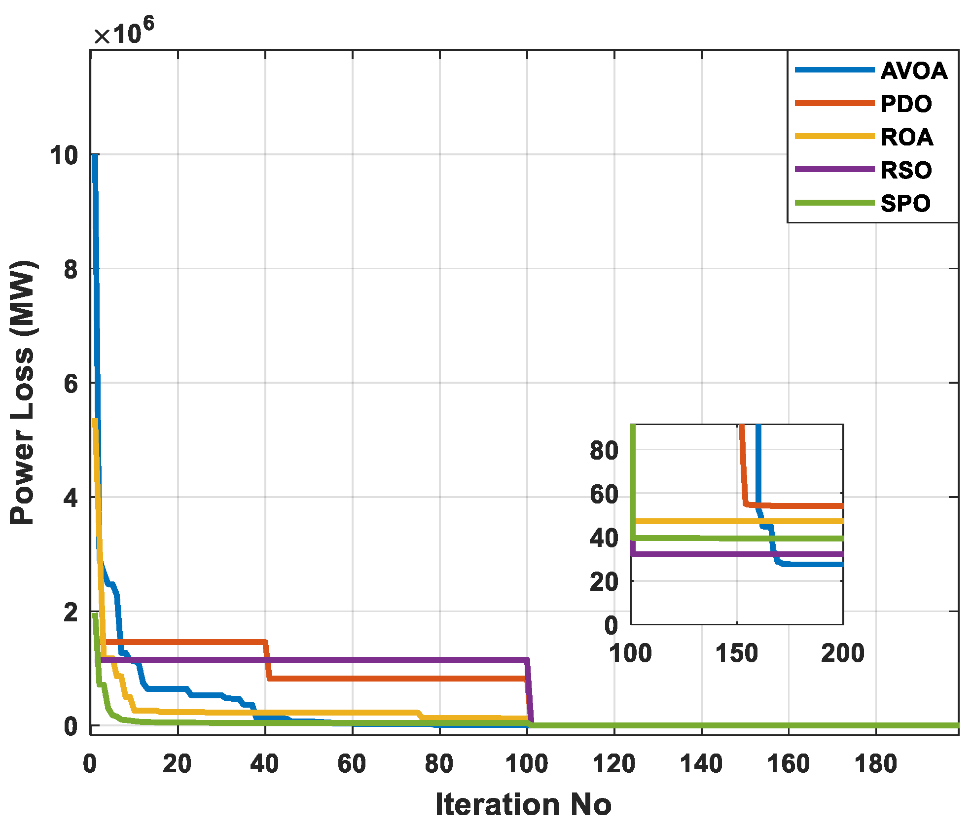
4.1.3. Case 3: Minimization of Transmission Power Losses in IEEE 30 Bus
4.1.4. Case 4: Minimization of Transmission Power Loss for Standard IEEE 30 Bus Incorporating RES
4.1.5. Case 5: Minimization of Multi-Objective Functions (Voltage-Level Deviation, Operational Cost, and Transmission Power Loss) with Continuous Control Variable Settings in IEEE-30 Bus
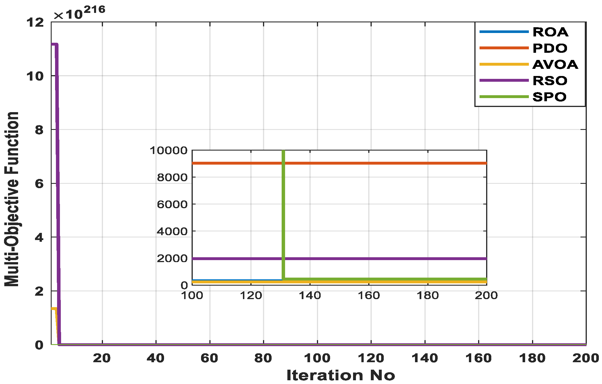
4.1.6. Case 6: Minimization of Multi-Objective Functions (Voltage-Level Deviation, Operational Cost, and Transmission Power Loss) with Discrete Control Variable Settings in IEEE-30 Bus
4.2. Standard IEEE-57 Bus Test System
4.2.1. Case 7: Minimization of Transmission Power Loss in IEEE 57 Bus
4.2.2. Case 8: Minimization of Transmission Power Loss for Standard IEEE 57 Bus Incorporating RES
4.3. Standard IEEE-118 Bus Test System
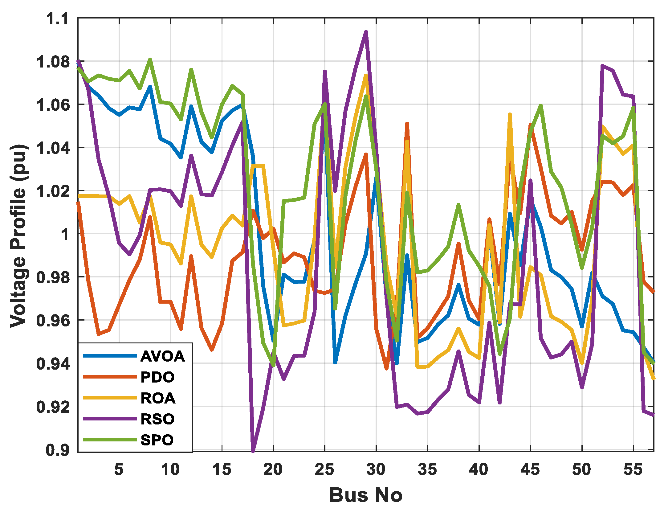
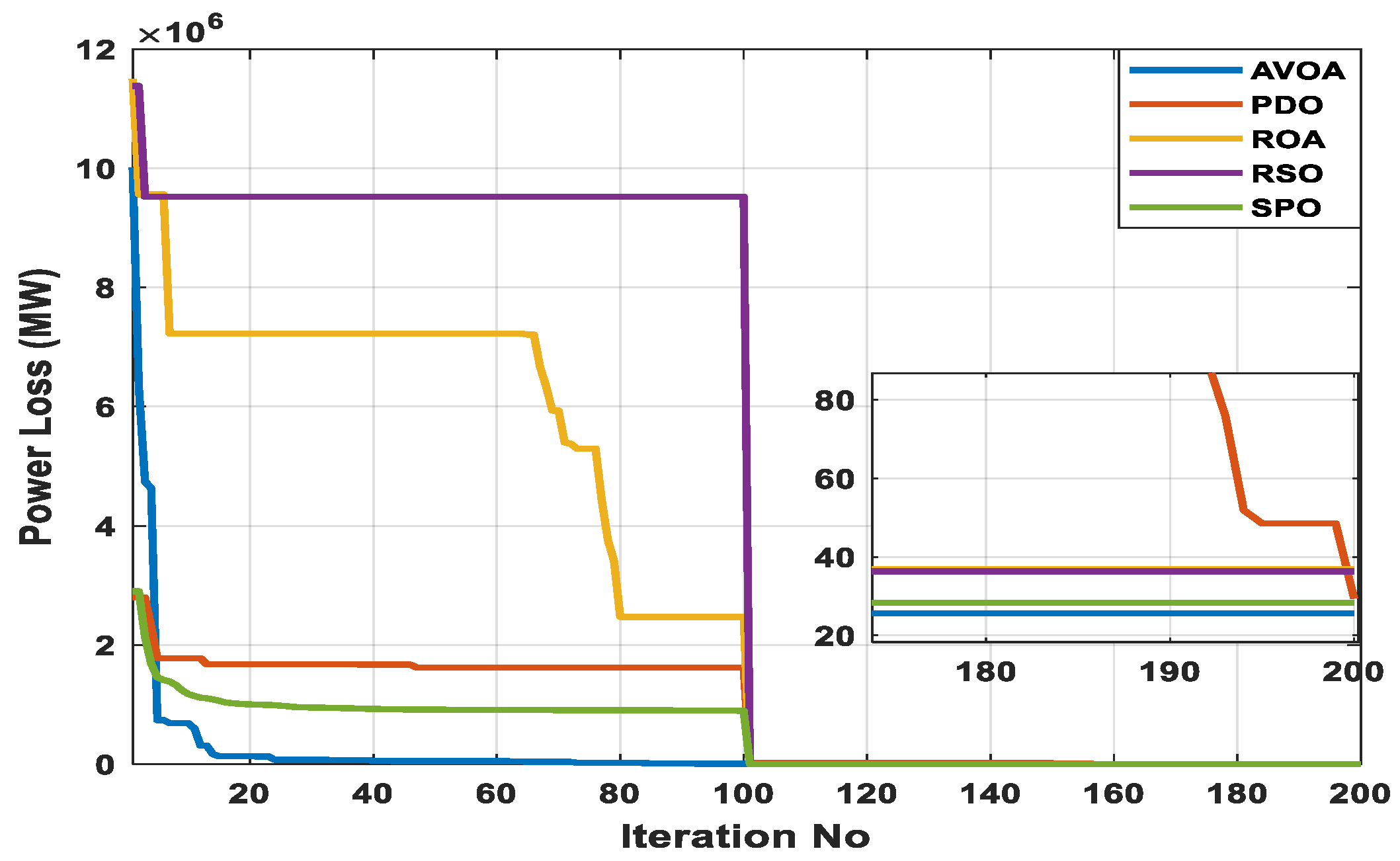
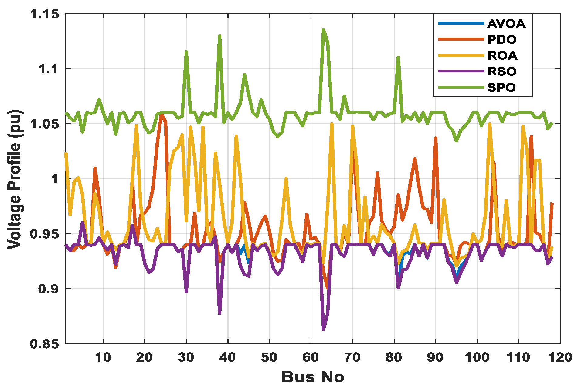
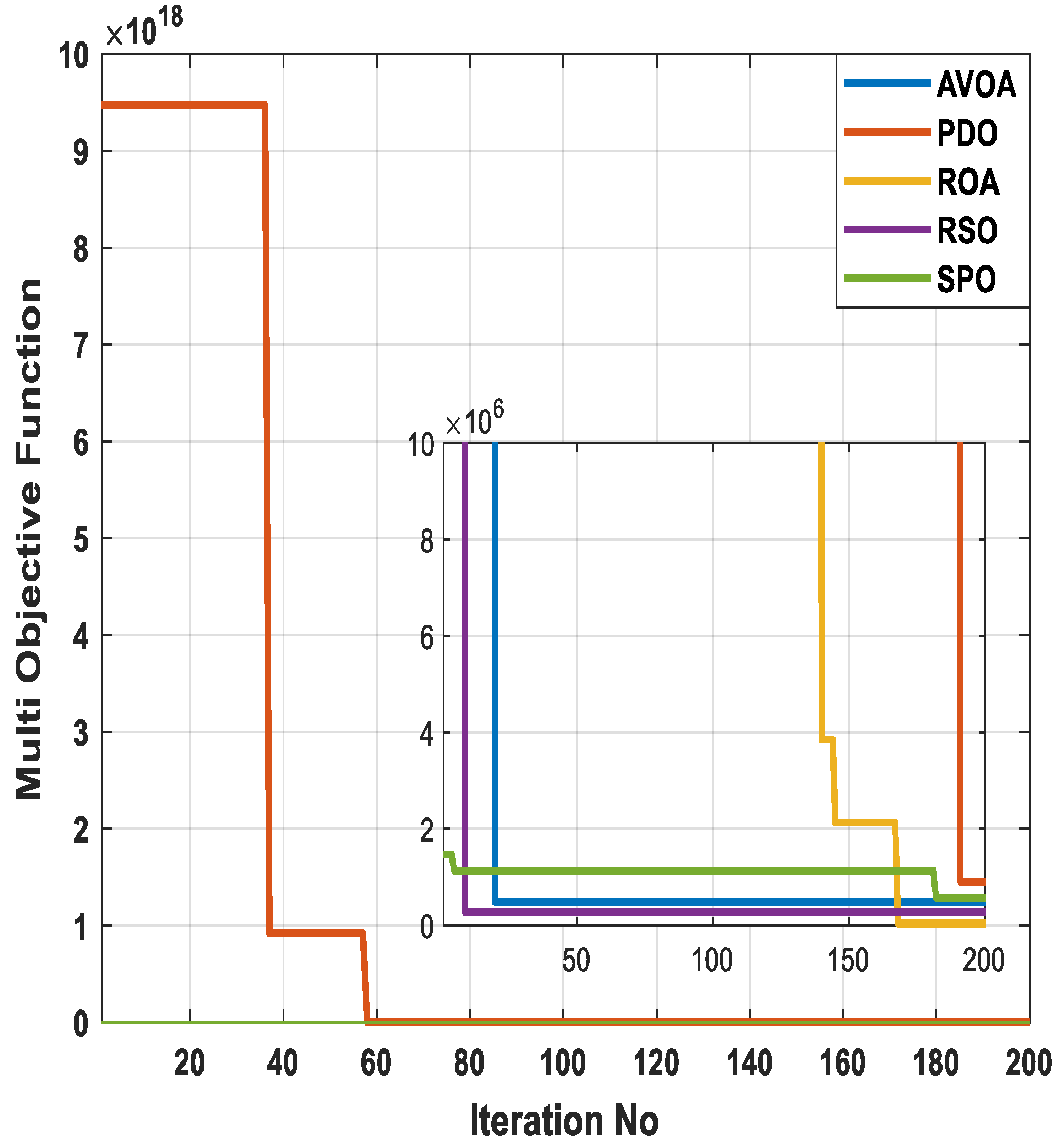
4.3.1. Case 9: Minimization of Multi-Objective Functions (Voltage-Level Deviation, Operational Cost, and Transmission Power Loss) with Continuous Control Variable Settings in IEEE-118 Bus
4.3.2. Case 10: Minimization of Multi-Objective Functions (Voltage-Level Deviation, Operational Cost, and Transmission Power Loss) with Discrete Control Variable Settings in IEEE-118 Bus
5. Conclusions
Author Contributions
Funding
Conflicts of Interest
Abbreviations
| A-CSOS | Adaptive chaotic symbiotic organisms search algorithm |
| AMOAIA | Adaptive multi-objective optimization artificial immune algorithm |
| AO | A novel Optimizer |
| AVOA | African Vultures Optimization Algorithm |
| CTFWO | Chaotic turbulent flow of water-based optimization algorithm |
| CA | Coot Algorithm |
| CBA | Chaotic bat algorithm |
| DP | Dynamic programming |
| EP | Evolutionary Programming |
| FA | Firefly Algorithm |
| FO-DPSO | Fractional-order Darwinian particle swarm optimization |
| FPSOGSA | Fractional particle swarm optimization-gravitational search algorithm |
| GWO | Grey wolf optimization algorithm |
| GWFA | Adaptive Grey Wolf-based Firefly Algorithm |
| HPSOFA | Hybridization of particle swarm optimization with firefly algorithm |
| HPSOBA | Hybrid bat optimization algorithm based on particle swarm algorithm |
| ICOA | Improved coyote optimization algorithm |
| IDE | Improved Differential evolution algorithm |
| IHBO | Improved Heap-based optimizer |
| IMPA | Improved Marine Predators Algorithm |
| IMFO | Improved Moth-flame Optimization algorithm |
| IPM | Interior Point Method |
| IRCGA | Improved real-coded genetic algorithm |
| IALO | Improved Antlion optimization algorithm |
| ICOA | Improved coyote optimization algorithm |
| ISSO | Improved social spider optimization |
| LAPO | Lightning attachment procedure optimization |
| LP | Linear Programming |
| MOPSO | Multi-objective particle swarm optimization algorithm |
| MPA | Marine predators’ algorithm |
| MPFA | Modified pathfinder algorithm |
| MSCA | Modified sine cosine algorithm |
| MVMO | Mean-variance mapping optimization algorithm |
| ORPD | Optimal reactive power dispatch |
| OF | Objective Function |
| PSO | Particle Swarm Optimization |
| PCA-RCGA | Real coded genetic algorithm with Principal component analysis |
| Ploss | Active power losses |
| QP | Quadratic Programming |
| RERs | Renewable energy resources |
| SCA | Sine-cosine algorithm |
| SMA | Slime mold algorithm |
| TVD | Total voltage deviation |
| VAR | Volt ampere reactive |
| WWO | Water wave optimization algorithm |
| Symbols | |
| First best vulture | |
| Second best vulture | |
| Function | |
| Conductance between bus and bus | |
| Susceptance between bus and bus | |
| Weight factor for objective function | |
| Equality constraints | |
| Inequality constraints | |
| Equality constraints numbers | |
| Inequality constraints numbers | |
| IEEE | Institute of Electrical and Electronics Engineers |
| The probability parameter for deciding the best vulture | |
| The probability parameter for deciding the second-best vulture | |
| The lower search spaces bound | |
| The upper search spaces bound | |
| Maximum iterations’ number | |
| Shunt compensator bank units’ numbers | |
| Generation buses numbers | |
| Load buses numbers | |
| Transformers numbers | |
| Number of transmission lines | |
| Vulture position vector | |
| A parameter that determines the chances of choosing a mechanism during the exploration phase | |
| A parameter that determines the chances of choosing a mechanism during the exploration phase of the first part | |
| A parameter that determines the chances of choosing mechanisms during the exploration phase of the second part | |
| Vultures’ numbers | |
| Slack bus power | |
| Generated active power at bus | |
| Generated reactive power at bus | |
| Demand active power at bus | |
| Demand reactive power at bus | |
| Injected reactive power of the shunt compensator | |
| Generator’s output reactive power | |
| A random number | |
| One of the top vultures selected | |
| The transmission line’s apparent power flow | |
| Transformer’s tap setting | |
| Control variables | |
| Generation bus voltage | |
| Load bus voltage | |
| Reference voltage | |
| State variables | |
| A parameter that defines the disruption of the exploration and exploitation phases | |
| USD/h | Dollar/hour |
| The phase difference of voltages |
References
- Yalcin, E.; Taplamacioglu, M.C.; Cam, E. The Adaptive Chaotic Symbiotic Organisms Search Algorithm Proposal for Optimal Reactive Power Dispatch Problem in Power Systems. Electrica 2019, 19, 37–47. [Google Scholar] [CrossRef]
- Muhammad, Y.; Khan, R.; Ullah, F.; Rehman, A.U.; Aslam, M.S.; Raja, M.A.Z. Design of fractional swarming strategy for solution of optimal reactive power dispatch. Neural Comput. Appl. 2020, 32, 10501–10518. [Google Scholar] [CrossRef]
- Gafar, M.G.; El-Sehiemy, R.A.; Hasanien, H.M. A Novel Hybrid Fuzzy-JAYA Optimization Algorithm for Efficient ORPD Solution. IEEE Access 2019, 7, 182078–182088. [Google Scholar] [CrossRef]
- Salimin, R.H.; Musirin, I.; Hamid, Z.A.; Harun, A.F.; Suliman, S.I.; Suyono, H.; Hasanah, R.N. Multi cases optimal reactive power dispatch using evolutionary programming. Indones. J. Electr. Eng. Comput. Sci. 2020, 17, 662–670. [Google Scholar] [CrossRef]
- ElSayed, S.; Elattar, E. Slime Mold Algorithm for Optimal Reactive Power Dispatch Combining with Renewable Energy Sources. Sustainability 2021, 13, 5831. [Google Scholar] [CrossRef]
- Mugemanyi, S.; Qu, Z.; Rugema, F.X.; Dong, Y.; Bananeza, C.; Wang, L. Optimal Reactive Power Dispatch Using Chaotic Bat Algorithm. IEEE Access 2020, 8, 65830–65867. [Google Scholar] [CrossRef]
- Jamal, R.; Men, B.; Khan, N.H. A Novel Nature Inspired Meta-Heuristic Optimization Approach of GWO Optimizer for Optimal Reactive Power Dispatch Problems. IEEE Access 2020, 8, 202596–202610. [Google Scholar] [CrossRef]
- Chaitanya, S.N.V.S.K.; Bakkiyaraj, R.A.; Rao, B.V. Technical Review on Optimal Reactive Power Dispatch with FACTS Devices and Renewable Energy Sources. In Lecture Notes in Electrical Engineering; Springer: Berlin/Heidelberg, Germany, 2022; Volume 766, pp. 185–194. [Google Scholar] [CrossRef]
- Pattanaik, J.K.; Basu, M.; Dash, D.P. Improved Real-Coded Genetic Algorithm for Reactive Power Dispatch. IETE J. Res. 2022, 68, 1462–1474. [Google Scholar] [CrossRef]
- Abdel-Fatah, S.; Ebeed, M.; Kamel, S. Optimal Reactive Power Dispatch Using Modified Sine Cosine Algorithm. Proceedings of 2019 International Conference on Innovative Trends in Computer Engineering (ITCE), Aswan, Egypt, 2–4 February 2019; pp. 510–514. [Google Scholar] [CrossRef]
- Li, Z.; Cao, Y.; Van Dai, L.; Yang, X.; Nguyen, T.T. Finding Solutions for Optimal Reactive Power Dispatch Problem by a Novel Improved Antlion Optimization Algorithm. Energies 2019, 12, 2968. [Google Scholar] [CrossRef]
- Nguyen, T.T.; Vo, D.N. Improved social spider optimization algorithm for optimal reactive power dispatch problem with different objectives. Neural Comput. Appl. 2020, 32, 5919–5950. [Google Scholar] [CrossRef]
- Saraswat, A.; Ucheniya, R.; Gupta, Y. Two-Stage Stochastic Optimization for Reactive Power Dispatch with Wind Power Uncertainties. In Proceedings of the International Conference on Computation, Automation and Knowledge Management (ICCAKM-2020), Dubai, United Arab Emirates, 9–10 January 2020; pp. 332–337. [Google Scholar] [CrossRef]
- Ebeed, M.; Ali, A.; Mosaad, M.I.; Kamel, S. An Improved Lightning Attachment Procedure Optimizer for Optimal Reactive Power Dispatch with Uncertainty in Renewable Energy Resources. IEEE Access 2020, 8, 168721–168731. [Google Scholar] [CrossRef]
- Jamal, R.; Men, B.; Khan, N.H.; Raja, M.A.Z.; Muhammad, Y. Application of Shannon Entropy Implementation Into a Novel Fractional Particle Swarm Optimization Gravitational Search Algorithm (FPSOGSA) for Optimal Reactive Power Dispatch Problem. IEEE Access 2021, 9, 2715–2733. [Google Scholar] [CrossRef]
- Khan, N.H.; Wang, Y.; Tian, D.; Raja, M.A.Z.; Jamal, R.; Muhammad, Y. Design of Fractional Particle Swarm Optimization Gravitational Search Algorithm for Optimal Reactive Power Dispatch Problems. IEEE Access 2020, 8, 146785–146806. [Google Scholar] [CrossRef]
- Khan, N.H.; Wang, Y.; Tian, D.; Jamal, R.; Ebeed, M.; Deng, Q. Fractional PSOGSA Algorithm Approach to Solve Optimal Reactive Power Dispatch Problems With Uncertainty of Renewable Energy Resources. IEEE Access 2020, 8, 215399–215413. [Google Scholar] [CrossRef]
- Kunapareddy, M.; Rao, B.V. Hybridization of Particle Swarm Optimization with Firefly Algorithm for Multi-objective Optimal Reactive Power Dispatch. In Lecture Notes in Mechanical Engineering; Springer: Berlin/Heidelberg, Germany, 2020; pp. 673–682. [Google Scholar] [CrossRef]
- Das, T.; Roy, R.; Mandal, K.K. Impact of the penetration of distributed generation on optimal reactive power dispatch. Prot. Control. Mod. Power Syst. 2020, 5, 1–26. [Google Scholar] [CrossRef]
- Yapici, H. Solution of optimal reactive power dispatch problem using pathfinder algorithm. Eng. Optim. 2021, 53, 1946–1963. [Google Scholar] [CrossRef]
- Zhou, Y.; Zhang, J.; Yang, X.; Ling, Y. Optimal reactive power dispatch using water wave optimization algorithm. Oper. Res. 2020, 20, 2537–2553. [Google Scholar] [CrossRef]
- Roy, R.; Das, T.; Mandal, K.K. Optimal Reactive Power Dispatch for Voltage Security using JAYA Algorithm. In Proceedings of the 2020 International Conference on Convergence to Digital World—Quo Vadis, ICCDW, Mumbai, India, 18–20 February 2020; pp. 1–6. [Google Scholar] [CrossRef]
- Ebeed, M.; Alhejji, A.; Kamel, S.; Jurado, F. Solving the Optimal Reactive Power Dispatch Using Marine Predators Algorithm Considering the Uncertainties in Load and Wind-Solar Generation Systems. Energies 2020, 13, 4316. [Google Scholar] [CrossRef]
- Ahmed, M.; Osman, M.; Korovkin, N. Optimal reactive power dispatch in power system comprising renewable energy sources by means of a multi-objective particle swarm algorithm. Mater. Sci. Power Eng. 2021, 27, 5–20. [Google Scholar] [CrossRef]
- Elsayed, S.K.; Kamel, S.; Selim, A.; Ahmed, M. An Improved Heap-Based Optimizer for Optimal Reactive Power Dispatch. IEEE Access 2021, 9, 58319–58336. [Google Scholar] [CrossRef]
- Londono, D.; Acevedo, W.V.; Camilo, D.; Tamayo, L.; María, J.; Lezama, L.; Mauricio, W.; Acevedo, V. Mean-Variance Mapping Optimization Algorithm Applied to the Optimal Reactive Power Dispatch. In INGE CUC; Universidad de la Costa-CUC: Barranquilla, Colombia, 2021; Volume 17. [Google Scholar] [CrossRef]
- Das, T.; Roy, R.; Mandal, K.K. Integrated PV system with Optimal Reactive Power Dispatch for Voltage Security using JAYA Algorithm. In Proceedings of the 7th International Conference on Electrical Energy Systems, ICEES, Chennai, India, 11–19 February 2021; pp. 56–61. [Google Scholar] [CrossRef]
- Das, T.; Roy, R.; Mandal, K.K. Solving Optimal Reactive Power Dispatch Problem with the Consideration of Load Uncertainty using Modified JAYA Algorithm. In Proceedings of the 2021 1st International Conference on Advances in Electrical, Computing, Communications and Sustainable Technologies, ICAECT, Bhilai, India, 19–20 February 2021; pp. 1–6. [Google Scholar] [CrossRef]
- Roy, R.; Das, T.; Mandal, K.K. Optimal reactive power dispatch using a novel optimization algorithm. J. Electr. Syst. Inf. Technol. 2021, 8, 18. [Google Scholar] [CrossRef]
- Hassan, M.H.; Kamel, S.; El-Dabah, M.A.; Khurshaid, T.; Dominguez-Garcia, J.L. Optimal Reactive Power Dispatch with Time-Varying Demand and Renewable Energy Uncertainty Using Rao-3 Algorithm. IEEE Access 2021, 9, 23264–23283. [Google Scholar] [CrossRef]
- Kien, L.; Hien, C.; Nguyen, T. Optimal Reactive Power Generation for Transmission Power Systems Considering Discrete Values of Capacitors and Tap Changers. Appl. Sci. 2021, 11, 5378. [Google Scholar] [CrossRef]
- Sabir, M.; Ahmad, A.; Ahmed, A.; Siddique, S.; Hashmi, U.A. A Modified Inertia Weight Control of Particle Swarm Optimization for Optimal Reactive Power Dispatch Problem. In Proceedings of the 2021 International Conference on Emerging Power Technologies, ICEPT, Topi, Pakistan, 10–11 April 2021; pp. 1–6. [Google Scholar] [CrossRef]
- Chi, R.; Li, Z.; Chi, X.; Qu, Z.; Tu, H.-B. Reactive Power Optimization of Power System Based on Improved Differential Evolution Algorithm. Math. Probl. Eng. 2021, 2021, 6690924. [Google Scholar] [CrossRef]
- Wahab, A.M.A.-E.; Kamel, S.; Hassan, M.H.; Mosaad, M.I.; AbdulFattah, T.A. Optimal Reactive Power Dispatch Using a Chaotic Turbulent Flow of Water-Based Optimization Algorithm. Mathematics 2022, 10, 346. [Google Scholar] [CrossRef]
- Shareef, S.K.M.; Rao, R.S. Adaptive Grey Wolf based on Firefly algorithm technique for optimal reactive power dispatch in unbalanced load conditions. J. Curr. Sci. Technol. 2019, 12, 11–31. [Google Scholar] [CrossRef]
- Ramkee, P.; Chaitanya, S.N.V.S.K.; Rao, B.V.; Bakkiyaraj, R.A. Optimal Reactive Power Dispatch Under Load Uncertainty Incorporating Solar Power Using Firefly Algorithm. In Lecture Notes in Electrical Engineering; Springer: Berlin/Heidelberg, Germany, 2022; pp. 423–434. [Google Scholar] [CrossRef]
- Khan, N.H.; Jamal, R.; Ebeed, M.; Kamel, S.; Zeinoddini-Meymand, H.; Zawbaa, H.M. Adopting Scenario-Based approach to solve optimal reactive power Dispatch problem with integration of wind and solar energy using improved Marine predator algorithm. Ain Shams Eng. J. 2022, 13, 101726. [Google Scholar] [CrossRef]
- Qin, L.; Xu, T.; Li, S.; Chen, Z.; Zhang, Q.; Tian, J.; Lin, Y. Coot Algorithm for Optimal Carbon–Energy Combined Flow of Power Grid with Aluminum Plants. Front. Energy Res. 2022, 10, 856314. [Google Scholar] [CrossRef]
- Sakthivel Padaiyatchi, S.; Jaya, S. Hybrid Bat Optimization Algorithm Applied to Optimal Reactive Power Dispatch Problems. Int. J. Electr. Electron. Eng. 2022, 9, 1–5. [Google Scholar] [CrossRef]
- Saddique, M.S.; Habib, S.; Haroon, S.S.; Bhatti, A.R.; Amin, S.; Ahmed, E.M. Optimal Solution of Reactive Power Dispatch in Transmission System to Minimize Power Losses Using Sine-Cosine Algorithm. IEEE Access 2022, 10, 20223–20239. [Google Scholar] [CrossRef]
- Lian, L. Reactive power optimization based on adaptive multi-objective optimization artificial immune algorithm. Ain Shams Eng. J. 2022, 13, 101677. [Google Scholar] [CrossRef]
- Zhang, M.; Li, Y. Multi-Objective Optimal Reactive Power Dispatch of Power Systems by Combining Classification-Based Multi-Objective Evolutionary Algorithm and Integrated Decision Making. IEEE Access 2020, 8, 38198–38209. [Google Scholar] [CrossRef]
- Muhammad, Y.; Khan, R.; Raja, M.A.Z.; Ullah, F.; Chaudhary, N.I.; He, Y. Solution of optimal reactive power dispatch with FACTS devices: A survey. Energy Rep. 2020, 6, 2211–2229. [Google Scholar] [CrossRef]
- Khan, N.H.; Wang, Y.; Tian, D.; Jamal, R.; Kamel, S.; Ebeed, M. Optimal Siting and Sizing of SSSC Using Modified Salp Swarm Algorithm Considering Optimal Reactive Power Dispatch Problem. IEEE Access 2021, 9, 49249–49266. [Google Scholar] [CrossRef]
- Niu, M.; Xu, N.Z.; Dong, H.N.; Ge, Y.Y.; Liu, Y.T.; Ngin, H.T. Adaptive Range Composite Differential Evolution for Fast Optimal Reactive Power Dispatch. IEEE Access 2021, 9, 20117–20126. [Google Scholar] [CrossRef]
- Li, Y.; Sun, B.; Zeng, Y.; Dong, S.; Ma, S.; Zhang, X. Active distribution network active and reactive power coordinated dispatching method based on discrete monkey algorithm. Int. J. Electr. Power Energy Syst. 2022, 14, 1084253. [Google Scholar] [CrossRef]
- Sun, B.; Jing, R.; Zeng, Y.; Li, Y.; Chen, J.; Liang, G. Distributed optimal dispatching method for smart distribution network considering effective interaction of source-network-load-storage flexible resources. Energy Rep. 2023, 9, 148–162. [Google Scholar] [CrossRef]
- Abdollahzadeh, B.; Gharehchopogh, F.S.; Mirjalili, S. African vultures optimization algorithm: A new nature-inspired metaheuristic algorithm for global optimization problems. Comput. Ind. Eng. 2021, 158, 107408. [Google Scholar] [CrossRef]
- Villa-Acevedo, W.M.; López-Lezama, J.M.; Valencia-Velásquez, J.A. A Novel Constraint Handling Approach for the Optimal Reactive Power Dispatch Problem. Energies 2018, 11, 2352. [Google Scholar] [CrossRef]
- Mouassa, S.; Bouktir, T.; Salhi, A. Ant lion optimizer for solving optimal reactive power dispatch problem in power systems. Eng. Sci. Technol. Int. J. 2017, 20, 885–895. [Google Scholar] [CrossRef]
- Nagarajan, K.; Parvathy, A.K.; Rajagopalan, A. Multi-Objective Optimal Reactive Power Dispatch using Levy Interior Search Algorithm. Int. J. Electr. Eng. Inform. 2020, 12, 547–570. [Google Scholar] [CrossRef]


| Research References | Year | Applied Methodology for ORPD Solution | Validation Test System | Optimization Objectives | |||||||||||
|---|---|---|---|---|---|---|---|---|---|---|---|---|---|---|---|
| Benchmark Functions | IEEE 14—Bus System | IEEE 30—Bus System | IEEE 39—Bus System | IEEE 57—Bus System | IEEE 118—Bus System | IEEE 300—Bus System | Active Power Losses Minimization | Voltage Deviation Minimization | Voltage Stability Index Improvement | Cost Minimization | Emission Minimization | Uncertainty Impact | |||
| [1] | 2019 | (A-CSOS) | √ | √ | √ | ||||||||||
| [2] | 2020 | (FO-DPSO) | √ | √ | √ | √ | |||||||||
| [3] | 2019 | Hybrid fuzzy-JAYA optimization algorithm | √ | √ | √ | √ | √ | ||||||||
| [4] | 2019 | (EP) | √ | √ | |||||||||||
| [5] | 2021 | (SMA) | √ | √ | √ | √ | √ | √ | √ | ||||||
| [6] | 2020 | (CBA) | √ | √ | √ | √ | √ | √ | √ | √ | |||||
| [7] | 2020 | (GWO) algorithm | √ | √ | √ | √ | √ | ||||||||
| [9] | 2019 | (IRCGA) | √ | √ | √ | √ | √ | √ | √ | ||||||
| [10] | 2019 | (MSCA) | √ | √ | √ | √ | |||||||||
| [11] | 2019 | (IALO) | √ | √ | √ | √ | √ | √ | |||||||
| [12] | 2020 | (ISSO) | √ | √ | √ | √ | √ | ||||||||
| [13] | 2020 | (PCA-RCGA) | √ | √ | √ | ||||||||||
| [14] | 2020 | (LAPO) | √ | √ | √ | √ | |||||||||
| [15] | 2020 | (FPSOGSA) | √ | √ | √ | √ | |||||||||
| [16] | 2020 | (FPSOGSA) | √ | √ | √ | √ | |||||||||
| [17] | 2020 | (FPSOGSA) | √ | √ | √ | √ | √ | ||||||||
| [18] | 2020 | (HPSOFA) | √ | √ | √ | √ | |||||||||
| [19] | 2020 | JAYA algorithm | √ | √ | √ | √ | √ | √ | |||||||
| [20] | 2020 | (MPFA) | √ | √ | √ | ||||||||||
| [21] | 2020 | (WWO) algorithm | √ | √ | |||||||||||
| [22] | 2020 | JAYA algorithm | √ | √ | √ | √ | |||||||||
| [23] | 2020 | (MPA) | √ | √ | √ | √ | |||||||||
| [24] | 2021 | (MOPSO) algorithm | √ | √ | √ | √ | √ | ||||||||
| [25] | 2021 | (IHBO) | √ | √ | √ | √ | √ | √ | |||||||
| [26] | 2021 | (MVMO) algorithm | √ | √ | √ | ||||||||||
| [27] | 2021 | JAYA algorithm | √ | √ | √ | √ | √ | ||||||||
| [28] | 2021 | Modified JAYA algorithm | √ | √ | √ | √ | √ | ||||||||
| [29] | 2021 | JAYA algorithm | √ | √ | √ | √ | √ | ||||||||
| [30] | 2021 | Rao-3 Algorithm | √ | √ | √ | √ | √ | √ | |||||||
| [31] | 2021 | (ICOA) | √ | √ | √ | √ | √ | √ | |||||||
| [32] | 2021 | A Modified Inertia Weight of Particle Swarm Optimization (PSO) | √ | √ | √ | ||||||||||
| [33] | 2021 | (IDE) algorithm | √ | √ | √ | √ | |||||||||
| [34] | 2022 | (CTFWO) algorithm | √ | √ | √ | √ | |||||||||
| [35] | 2022 | (GWFA) | √ | √ | √ | √ | √ | ||||||||
| [36] | 2022 | (FA) | √ | √ | √ | √ | |||||||||
| [37] | 2022 | (IMPA) | √ | √ | √ | √ | √ | ||||||||
| [38] | 2022 | Coot Algorithm (CA) | √ | √ | √ | √ | |||||||||
| [39] | 2022 | (HPSOBA) | √ | √ | √ | √ | |||||||||
| [40] | 2022 | (SCA) | √ | √ | √ | √ | |||||||||
| [41] | 2022 | (AMOAIA) | √ | √ | √ | √ | |||||||||
| Algorithm | Parameters | Value |
|---|---|---|
| AVOA | 0.8 | |
| 0.2 | ||
| 2.5 | ||
| 0.6 | ||
| 0.4 | ||
| 0.6 |
| Case No | Objective Function |
|---|---|
| 1 | Minimization of voltage-level deviation in IEEE-30 bus. |
| 2 | Minimization of operational cost in IEEE-30 bus. |
| 3 | Minimization of transmission power loss in IEEE-30 bus. |
| 4 | Minimization of transmission power loss incorporating optimal renewable energy sources in IEEE-30 bus. |
| 5 | Minimization of multi-objective functions (voltage-level deviation, operational cost, and transmission power loss) with continuous control variable settings in IEEE-30 bus. |
| 6 | Minimization of multi-objective functions (voltage-level deviation, operational cost, and transmission power loss) with discrete control variable settings in IEEE-30 bus. |
| 7 | Minimization of transmission power loss in IEEE-57 bus. |
| 8 | Minimization of transmission power loss incorporating optimal renewable energy sources in IEEE-57 bus. |
| 9 | Minimization of multi-objective functions (voltage-level deviation, operational cost, and transmission power loss) with continuous control variable settings in IEEE-118 bus. |
| 10 | Minimization of multi-objective functions (voltage-level deviation, operational cost, and transmission power loss) with discrete control variable settings in IEEE-118 bus. |
| Parameters | 30-Bus | 57-Bus | 118-Bus |
|---|---|---|---|
| Control variable numbers | 19 | 25 | 77 |
| Generator numbers | 6 | 7 | 45 |
| Transformer Tap numbers | 4 | 15 | 9 |
| Q-shunt numbers | 9 | 3 | 14 |
| Parameters | Variables | Min-Value | Max-Value | Step Size |
|---|---|---|---|---|
| 30-Bus | 0.95 | 1.1 | Continuous | |
| 0.9 | 1.1 | 0.01 (20-level) | ||
| 0 | 5MVAR | 0.05 (100-step) | ||
| 57-Bus | 0.9 | 1.1 | Continuous | |
| 0.9 | 1.1 | Continuous | ||
| 0 | 30MVAR | Continuous | ||
| 118-Bus | 0.94 | 1.06 | Continuous | |
| 0.9 | 1.1 | 0.01 (20-level) | ||
| 0 | 30MVAR | 0.3 (100-step) |
| Control Variables | PDO | RSO | AVOA | ROA | SPO |
|---|---|---|---|---|---|
| (pu) | 1.023328 | 1.049871 | 1.008875 | 1.011852 | 1.037673 |
| (pu) | 1.008159 | 1.036918 | 1.003797 | 1.008226 | 1.040367 |
| (pu) | 1.000557 | 1.010459 | 1.018456 | 1.003649 | 1.025815 |
| (pu) | 0.994860 | 0.985178 | 0.999638 | 1.006250 | 0.994378 |
| (pu) | 1.082926 | 0.975178 | 1.087355 | 1.013930 | 0.992829 |
| (pu) | 1.008800 | 1.092579 | 1.005192 | 0.997207 | 1.001126 |
| (6-9) | 1.047965 | 1.051309 | 1.090717 | 0.973667 | 0.997475 |
| (6-10) | 0.921887 | 0.927919 | 0.919338 | 0.973680 | 0.900000 |
| (4-12) | 0.984708 | 1.012708 | 0.974276 | 0.973665 | 0.939858 |
| (28-27) | 0.937218 | 0.926008 | 0.965334 | 0.973737 | 0.939329 |
| (MVAR) | 5.000000 | 4.398053 | 2.184212 | 5.000000 | 2.368492 |
| (MVAR) | 5.000000 | 0.429754 | 4.994771 | 5.000000 | 1.280472 |
| (MVAR) | 5.000000 | 3.127819 | 3.855124 | 5.000000 | 1.006742 |
| (MVAR) | 0.000000 | 3.826915 | 4.686445 | 5.000000 | 1.237033 |
| (MVAR) | 4.456893 | 4.590043 | 4.986836 | 5.000000 | 5.000000 |
| (MVAR) | 5.000000 | 4.029262 | 4.267873 | 5.000000 | 4.746975 |
| (MVAR) | 5.000000 | 2.063050 | 4.507320 | 5.000000 | 3.478525 |
| (MVAR) | 0.000000 | 1.468192 | 4.999888 | 5.000000 | 4.288032 |
| (MVAR) | 0.000000 | 3.338243 | 2.533782 | 5.000000 | 0.000000 |
| Power Losses (MW) | 5.502730 | 5.789450 | 5.794690 | 5.627020 | 5.815130 |
| Voltage Deviation (pu) | 0.141010 | 0.293620 | 0.103090 | 0.126710 | 0.124770 |
| Method | Balance of Active Power | Balance of Reactive Power | ||||||
|---|---|---|---|---|---|---|---|---|
| Load (MW) | Generation (MW) | Loss (MW) | Load (MVAR) | Generation (MVAR) | Shunt VAR Compensation (MVAR) | Shunt Admittance and Branch Charging (MVAR) | Loss (MVAR) | |
| PDO | 283.400 | 288.903 | 5.503 | 126.200 | 92.603 | 29.457 | 30.486 | 26.346 |
| RSO | 283.400 | 289.189 | 5.789 | 126.200 | 93.894 | 27.271 | 32.816 | 27.782 |
| AVOA | 283.400 | 289.195 | 5.795 | 126.200 | 88.998 | 37.016 | 28.309 | 28.123 |
| ROA | 283.400 | 289.027 | 5.627 | 126.200 | 72.498 | 45.000 | 33.133 | 24.431 |
| SPO | 283.400 | 289.215 | 5.815 | 126.200 | 96.332 | 23.406 | 31.325 | 24.863 |
| Method | Minimum Value | Maximum Value | Mean Value | Standard Deviation | Mean Value of Computational Time |
|---|---|---|---|---|---|
| PDO | 0.14101 | 225.70993 | 23.85192 | 60.80698 | 16.83349 (s) |
| RSO | 0.29362 | 1624.08688 | 194.90665 | 325.54255 | 42.39668 (s) |
| AVOA | 0.10309 | 0.2324700 | 0.150460 | 0.028750 | 18.85260 (s) |
| ROA | 0.12671 | 36.849600 | 5.888400 | 12.66745 | 100.80976 (s) |
| SPO | 0.12477 | 201.57414 | 6.740770 | 29.61497 | 119.25339 (s) |
| Control Variables | PDO | RSO | AVOA | ROA | SPO |
|---|---|---|---|---|---|
| (pu) | 1.077223 | 1.010074 | 1.078933 | 1.009823 | 1.096953 |
| (pu) | 1.062954 | 0.970207 | 1.040035 | 1.009823 | 1.093400 |
| (pu) | 1.034902 | 0.950000 | 0.997439 | 1.009860 | 1.100000 |
| (pu) | 0.987255 | 0.950000 | 0.950000 | 1.009823 | 1.036836 |
| (pu) | 0.966547 | 0.950000 | 0.988204 | 1.010017 | 1.100000 |
| (pu) | 1.058877 | 0.950000 | 1.013312 | 1.009823 | 1.100000 |
| (6-9) | 1.021251 | 1.004746 | 0.932451 | 0.972293 | 0.928126 |
| (6-10) | 0.958663 | 0.900000 | 0.930201 | 0.972293 | 0.964485 |
| (4-12) | 0.921516 | 0.900000 | 0.906104 | 0.947242 | 1.087568 |
| (28-27) | 0.973659 | 0.900000 | 0.954467 | 0.947285 | 0.943896 |
| (MVAR) | 5.000000 | 2.754954 | 0.000000 | 4.718844 | 5.000000 |
| (MVAR) | 5.000000 | 2.543246 | 0.324557 | 4.718844 | 4.977415 |
| (MVAR) | 0.000000 | 2.222816 | 0.118031 | 4.720256 | 0.000000 |
| (MVAR) | 0.000000 | 3.212513 | 4.210257 | 4.718844 | 5.000000 |
| (MVAR) | 5.000000 | 2.973234 | 4.581713 | 4.720256 | 0.318032 |
| (MVAR) | 5.000000 | 0.000000 | 0.000000 | 4.718844 | 1.081768 |
| (MVAR) | 5.000000 | 2.625242 | 0.000000 | 4.720256 | 5.000000 |
| (MVAR) | 0.000000 | 0.504981 | 0.574697 | 4.720256 | 1.921813 |
| (MVAR) | 5.000000 | 0.000000 | 5.000000 | 4.718844 | 3.431373 |
| Cost (USD/h) | 82.703420 | 351.212637 | 81.268916 | 150.071347 | 103.635994 |
| Power Losses (MW) | 6.597461 | 6.946435 | 7.964927 | 5.743704 | 5.777907 |
| Voltage Deviation (pu) | 0.299451 | 1.198932 | 0.383136 | 0.243850 | 1.518099 |
| Method | Balance of Active Power | Balance of Reactive Power | ||||||
|---|---|---|---|---|---|---|---|---|
| Load (MW) | Generation (MW) | Loss (MW) | Load (MVAR) | Generation (MVAR) | Shunt VAR Compensation (MVAR) | Shunt Admittance and Branch Charging (MVAR) | Loss (MVAR) | |
| PDO | 283.400 | 288.841 | 5.441 | 126.200 | 84.227 | 24.035 | 32.995 | 33.013 |
| RSO | 283.400 | 288.521 | 5.121 | 126.200 | 88.280 | 24.321 | 26.979 | 35.262 |
| AVOA | 283.400 | 288.793 | 5.393 | 126.200 | 86.205 | 23.382 | 31.356 | 32.021 |
| ROA | 283.400 | 288.820 | 5.420 | 126.200 | 82.678 | 24.221 | 34.025 | 33.718 |
| SPO | 283.400 | 288.674 | 5.274 | 126.200 | 84.765 | 23.216 | 32.154 | 32.497 |
| Method | Minimum Value | Maximum Value | Mean Value | Standard Deviation | Mean Value of Computational Time |
|---|---|---|---|---|---|
| PDO | 1006.71192 | 1517.74404 | 1162.93396 | 158.66803 | 23.09068 (s) |
| RSO | 1181.05238 | 3126.24346 | 1474.70360 | 329.13510 | 21.79979 (s) |
| AVOA | 972.25120 | 1078.00374 | 992.75867 | 22.999580 | 15.85748 (s) |
| ROA | 1015.93296 | 1215.87610 | 1109.35461 | 64.874550 | 98.75274 (s) |
| SPO | 991.15484 | 1648.76614 | 1143.98243 | 172.34129 | 78.69903 (s) |
| Control Variables | PDO | RSO | AVOA | ROA | SPO |
|---|---|---|---|---|---|
| (pu) | 1.073600 | 1.091200 | 1.100000 | 1.100000 | 1.100000 |
| (pu) | 1.063800 | 1.085800 | 1.094403 | 1.095900 | 1.095600 |
| (pu) | 1.039600 | 1.073700 | 1.074998 | 1.072400 | 1.075000 |
| (pu) | 1.041100 | 1.038700 | 1.076819 | 1.079600 | 1.077400 |
| (pu) | 1.098600 | 1.043100 | 1.099993 | 1.100000 | 1.100000 |
| (pu) | 1.094100 | 1.095400 | 1.100000 | 1.100000 | 1.099000 |
| (6-9) | 0.993800 | 0.962000 | 1.042528 | 1.025200 | 0.978500 |
| (6-10) | 0.966300 | 0.968800 | 0.900024 | 1.040200 | 0.988700 |
| (4-12) | 0.983100 | 1.036400 | 0.980079 | 1.028200 | 0.995900 |
| (28-27) | 0.954100 | 0.988300 | 0.966956 | 1.002600 | 0.976800 |
| (MVAR) | 5.000000 | 3.840300 | 4.659089 | 5.000000 | 4.073100 |
| (MVAR) | 5.000000 | 2.919700 | 3.784615 | 5.000000 | 0.440700 |
| (MVAR) | 0.000000 | 1.070700 | 4.998465 | 5.000000 | 4.977900 |
| (MVAR) | 5.000000 | 0.760800 | 4.976225 | 5.000000 | 5.000000 |
| (MVAR) | 0.000000 | 0.920200 | 4.843913 | 5.000000 | 5.000000 |
| (MVAR) | 5.000000 | 3.404000 | 4.877789 | 5.000000 | 3.665900 |
| (MVAR) | 4.062800 | 4.981000 | 4.678076 | 5.000000 | 4.254900 |
| (MVAR) | 5.000000 | 3.509100 | 4.983888 | 5.000000 | 4.322500 |
| (MVAR) | 0.000000 | 3.637300 | 2.469794 | 5.000000 | 2.833000 |
| Power Losses (MW) | 4.839510 | 5.132850 | 4.546470 | 4.627150 | 4.573080 |
| Voltage Deviation (pu) | 1.266310 | 1.024060 | 1.988920 | 1.586570 | 1.825720 |
| Method | Balance of Active Power | Balance of Reactive Power | ||||||
|---|---|---|---|---|---|---|---|---|
| Load (MW) | Generation (MW) | Loss (MW) | Load (MVAR) | Generation (MVAR) | Shunt VAR Compensation (MVAR) | Shunt Admittance and Branch Charging (MVAR) | Loss (MVAR) | |
| PDO | 283.400 | 288.240 | 4.840 | 126.200 | 82.622 | 29.063 | 36.897 | 22.382 |
| RSO | 283.400 | 288.533 | 5.133 | 126.200 | 87.795 | 25.043 | 36.383 | 23.021 |
| AVOA | 283.400 | 287.946 | 4.546 | 126.200 | 70.324 | 40.272 | 36.000 | 20.395 |
| ROA | 283.400 | 288.027 | 4.627 | 126.200 | 63.608 | 45.000 | 38.654 | 21.062 |
| SPO | 283.400 | 287.973 | 4.573 | 126.200 | 73.003 | 34.568 | 38.824 | 20.194 |
| Method | Minimum Value | Maximum Value | Mean Value | Standard Deviation | Mean Value of Computational Time |
|---|---|---|---|---|---|
| PDO | 4.840 | 16,002.689 | 1504.755 | 3986.054 | 46.108410 (s) |
| RSO | 5.133 | 17,6611.603 | 13,757.799 | 29,157.813 | 17.582580 (s) |
| AVOA | 4.546 | 4.708000 | 4.587000 | 0.042000 | 16.001850 (s) |
| ROA | 4.627 | 3531.414 | 519.6950 | 1172.257 | 108.32703 (s) |
| SPO | 4.573 | 22,390.582 | 1351.229 | 5029.313 | 79.124780 (s) |
| Control Variables | PDO | RSO | AVOA | ROA | SPO | |
|---|---|---|---|---|---|---|
| (pu) | 1.100000 | 1.099455 | 1.100000 | 1.097868 | 1.100000 | |
| (pu) | 1.099989 | 1.099851 | 1.097978 | 1.096221 | 1.094982 | |
| (pu) | 1.099587 | 1.024629 | 1.081564 | 1.085981 | 1.073478 | |
| (pu) | 1.093189 | 1.068854 | 1.088944 | 1.082906 | 1.077110 | |
| (pu) | 1.085935 | 1.019485 | 1.099938 | 1.095299 | 1.100000 | |
| (pu) | 1.012753 | 1.033458 | 1.100000 | 1.071204 | 1.100000 | |
| (6-9) | 1.099679 | 1.077608 | 0.988583 | 1.042668 | 1.013376 | |
| (6-10) | 1.099712 | 0.918801 | 0.958993 | 1.074469 | 1.028824 | |
| (4-12) | 1.099075 | 1.016538 | 0.988412 | 1.043277 | 1.010851 | |
| (28-27) | 1.090130 | 1.063849 | 0.984554 | 1.078806 | 0.984372 | |
| (MVAR) | 5.000000 | 2.367058 | 3.455445 | 2.682247 | 0.275218 | |
| (MVAR) | 5.000000 | 4.952253 | 4.950191 | 1.501447 | 4.670871 | |
| (MVAR) | 5.000000 | 2.472453 | 4.388203 | 3.121859 | 4.671834 | |
| (MVAR) | 5.000000 | 2.635213 | 4.167731 | 3.102620 | 3.951102 | |
| (MVAR) | 2.938907 | 4.859103 | 2.978210 | 1.318443 | 4.908250 | |
| (MVAR) | 5.000000 | 0.260195 | 5.000000 | 0.704469 | 1.595587 | |
| (MVAR) | 5.000000 | 2.101977 | 1.768431 | 3.208966 | 2.680394 | |
| (MVAR) | 5.000000 | 1.679141 | 4.453273 | 0.569255 | 4.916036 | |
| (MVAR) | 3.705237 | 0.630078 | 3.422900 | 2.628873 | 5.000000 | |
| RES Location and Size | Location | 21.00000 | 25.00000 | 28.00000 | 21.00000 | 21.00000 |
| MW | 46.35348 | 48.73839 | 46.07358 | 44.31754 | 46.19743 | |
| MVAR | 0.000000 | 6.568155 | 11.33584 | 11.81921 | 16.39360 | |
| Power Losses (MW) | 3.035540 | 4.980920 | 2.674380 | 3.040910 | 2.797390 | |
| Voltage Deviation (pu) | 0.691760 | 0.648760 | 2.064220 | 1.013430 | 1.897910 | |
| Method | Balance of Active Power | Balance of Reactive Power | ||||||||
|---|---|---|---|---|---|---|---|---|---|---|
| Load (MW) | Generation (MW) | RES (MW) | Loss (MW) | Load (MVAR) | Generation (MVAR) | RES (MVAR) | Shunt VAR Compensation (MVAR) | Shunt Admittance and Branch Charging (MVAR) | Loss (MVAR) | |
| PDO | 283.4 | 240.082 | 46.353 | 3.036 | 126.2 | 58.434 | 0.0000 | 41.644 | 47.542 | 21.419 |
| RSO | 283.4 | 239.643 | 48.738 | 4.981 | 126.2 | 80.243 | 6.5681 | 21.957 | 37.258 | 19.827 |
| AVOA | 283.4 | 240.001 | 46.073 | 2.674 | 126.2 | 54.796 | 11.335 | 34.584 | 38.962 | 13.478 |
| ROA | 283.4 | 242.123 | 44.317 | 3.041 | 126.2 | 69.091 | 11.819 | 18.838 | 41.999 | 15.547 |
| SPO | 283.4 | 240.000 | 46.197 | 2.797 | 126.2 | 49.402 | 16.393 | 32.669 | 38.566 | 10.831 |
| Method | Minimum Value | Maximum Value | Mean Value | Standard Deviation | Mean Value of Computational Time |
|---|---|---|---|---|---|
| PDO | 3.03600 | 23451.0380 | 4069.32700 | 6986.33300 | 23.117360 (s) |
| RSO | 4.98092 | 5587.77200 | 3635.62384 | 1459.32771 | 18.682660 (s) |
| AVOA | 2.67400 | 5.44200000 | 3.30300000 | 0.63700000 | 20.668900 (s) |
| ROA | 3.04100 | 707.269000 | 29.5230000 | 106.320000 | 188.90750 (s) |
| SPO | 2.79700 | 13072.7640 | 587.630000 | 2454.28500 | 83.338790 (s) |
| Control Variables | PDO | RSO | AVOA | ROA | SPO |
|---|---|---|---|---|---|
| (pu) | 1.034042 | 1.013040 | 1.096031 | 1.015558 | 1.099988 |
| (pu) | 1.000626 | 1.002160 | 1.070756 | 1.011386 | 1.088032 |
| (pu) | 0.950586 | 0.957289 | 1.028974 | 1.003144 | 1.067478 |
| (pu) | 0.954355 | 0.970801 | 0.982896 | 1.010000 | 1.023205 |
| (pu) | 1.030482 | 0.992876 | 0.997983 | 1.001603 | 1.093794 |
| (pu) | 1.080495 | 1.074294 | 0.994995 | 1.021175 | 0.981983 |
| (6-9) | 0.972125 | 0.946234 | 0.985301 | 0.970950 | 1.004438 |
| (6-10) | 0.979401 | 0.962047 | 0.901766 | 0.996247 | 0.959636 |
| (4-12) | 0.900002 | 0.935633 | 0.954967 | 0.989841 | 1.038180 |
| (28-27) | 0.934839 | 0.910310 | 0.966368 | 0.973880 | 1.016444 |
| (MVAR) | 0.000000 | 4.296961 | 0.373418 | 4.238483 | 2.887637 |
| (MVAR) | 0.000000 | 4.868191 | 4.655968 | 4.323851 | 0.000000 |
| (MVAR) | 0.000000 | 0.495375 | 1.635248 | 4.105074 | 1.799884 |
| (MVAR) | 0.000000 | 3.882412 | 4.359865 | 4.211507 | 1.983525 |
| (MVAR) | 5.000000 | 0.369930 | 1.755742 | 3.917401 | 4.822479 |
| (MVAR) | 2.731975 | 1.833711 | 2.966848 | 4.251728 | 4.552650 |
| (MVAR) | 0.000000 | 2.368489 | 4.552541 | 4.323851 | 4.999714 |
| (MVAR) | 5.000000 | 0.057049 | 4.277262 | 4.077535 | 3.441456 |
| (MVAR) | 4.884375 | 4.504252 | 3.904529 | 4.121847 | 4.479210 |
| Voltage Deviation (pu) | 0.396291 | 0.394974 | 0.178213 | 0.147804 | 0.435536 |
| Cost (USD/h) | 90.02432 | 88.97314 | 50.13732 | 80.29645 | 57.96144 |
| Power Losses (MW) | 6.620585 | 5.952060 | 6.891535 | 5.554982 | 5.844435 |
| Multi-objective function | 153.919925 | 157.098928 | 103.336931 | 138.203123 | 136.375579 |
| Control Variables | PDO | RSO | AVOA | ROA | SPO |
|---|---|---|---|---|---|
| (pu) | 0.950000 | 0.950000 | 1.013608 | 1.082459 | 1.100000 |
| (pu) | 0.950000 | 0.950000 | 1.013608 | 1.082459 | 1.100000 |
| (pu) | 0.950000 | 0.950000 | 1.013608 | 1.082459 | 1.100000 |
| (pu) | 0.950000 | 0.950000 | 1.013608 | 1.082459 | 1.100000 |
| (pu) | 0.950000 | 0.950000 | 1.013608 | 1.082459 | 1.100000 |
| (pu) | 0.950000 | 0.950000 | 1.013608 | 1.082459 | 1.100000 |
| (6-9) | 0.900000 | 0.900000 | 1.010000 | 1.030000 | 1.100000 |
| (6-10) | 0.900000 | 0.900000 | 1.010000 | 1.030000 | 1.100000 |
| (4-12) | 0.900000 | 0.900000 | 1.010000 | 1.030000 | 1.100000 |
| (28-27) | 1.100000 | 0.900000 | 1.010000 | 1.030000 | 1.100000 |
| (MVAR) | 0.000000 | 0.000000 | 4.600000 | 2.700000 | 5.000000 |
| (MVAR) | 0.000000 | 0.000000 | 4.600000 | 4.400000 | 4.850000 |
| (MVAR) | 0.000000 | 0.000000 | 4.600000 | 2.900000 | 5.000000 |
| (MVAR) | 2.200000 | 0.000000 | 4.600000 | 5.000000 | 0.000000 |
| (MVAR) | 0.000000 | 0.000000 | 4.600000 | 3.250000 | 5.000000 |
| (MVAR) | 0.000000 | 0.000000 | 4.600000 | 0.000000 | 1.300000 |
| (MVAR) | 0.200000 | 0.000000 | 4.600000 | 5.000000 | 5.000000 |
| (MVAR) | 0.000000 | 0.000000 | 4.600000 | 0.900000 | 0.700000 |
| (MVAR) | 0.000000 | 1.250000 | 4.600000 | 1.700000 | 5.000000 |
| Voltage Deviation (pu) | 2.136450 | 1.340780 | 0.322600 | 0.978970 | 0.914060 |
| Cost (USD/h) | 132.4474 | 133.1194 | 90.48282 | 78.08285 | 96.59046 |
| Power Losses (MW) | 7.937040 | 7.276330 | 5.648940 | 5.034010 | 5.117670 |
| Multi-objective function | 9036.805590 | 1952.706490 | 234.854930 | 330.749040 | 450.021300 |
| Control Variables | PDO | RSO | AVOA | ROA | SPO |
|---|---|---|---|---|---|
| (pu) | 1.014757 | 1.079382 | 1.080374 | 1.017385 | 1.076876 |
| (pu) | 0.978060 | 1.067958 | 1.066919 | 1.017385 | 1.070644 |
| (pu) | 0.953511 | 1.063965 | 1.034293 | 1.017385 | 1.073361 |
| (pu) | 0.978504 | 1.058594 | 0.990386 | 1.017385 | 1.075436 |
| (pu) | 1.007692 | 1.068161 | 1.020260 | 1.017385 | 1.080711 |
| (pu) | 0.968363 | 1.044105 | 1.020613 | 0.995944 | 1.061063 |
| (pu) | 0.989555 | 1.059060 | 1.036204 | 1.017385 | 1.076054 |
| (4-18) | 0.913049 | 1.003605 | 0.943555 | 1.017385 | 1.021544 |
| (4-18) | 0.900000 | 0.984822 | 1.085978 | 1.017385 | 1.076384 |
| (21-20) | 0.974656 | 1.068002 | 0.948072 | 0.971602 | 1.097143 |
| (24-25) | 0.908226 | 1.040848 | 0.940854 | 1.017385 | 1.090065 |
| (24-25) | 0.900001 | 1.069429 | 0.938419 | 1.017385 | 1.039761 |
| (24-26) | 1.001831 | 1.060441 | 0.946427 | 1.017385 | 1.094090 |
| (7-29) | 0.949960 | 1.065368 | 0.910877 | 0.929103 | 0.994970 |
| (34-32) | 0.969328 | 1.045765 | 1.043665 | 1.017385 | 1.072752 |
| (11-41) | 0.950228 | 0.961513 | 1.001356 | 0.971472 | 0.997184 |
| (15-45) | 0.900430 | 1.029488 | 0.979318 | 1.017385 | 1.008150 |
| (14-46) | 0.906230 | 1.022964 | 1.068994 | 0.997602 | 0.965880 |
| (10-51) | 0.947442 | 1.053327 | 1.067980 | 1.017385 | 1.051045 |
| (13-49) | 0.900006 | 1.048173 | 1.021711 | 1.017385 | 1.049060 |
| (11-43) | 0.911247 | 1.020260 | 1.040798 | 0.916027 | 1.099736 |
| (40-56) | 0.939646 | 1.024146 | 0.993105 | 1.005665 | 0.990529 |
| (39-57) | 0.963492 | 0.990351 | 0.954516 | 1.010802 | 1.020521 |
| (9-55) | 0.948951 | 1.099189 | 0.963165 | 0.958351 | 1.001199 |
| (MVAR) | 0.000000 | 8.482640 | 1.053096 | 21.99263 | 13.08836 |
| (MVAR) | 0.000000 | 26.36727 | 21.99351 | 21.99263 | 19.31112 |
| (MVAR) | 28.42860 | 27.78365 | 28.737910 | 21.992630 | 20.723070 |
| Power Losses (MW) | 50.57143 | 32.60550 | 27.51680 | 47.24557 | 39.26724 |
| Voltage Deviation(pu) | 1.280390 | 1.742980 | 2.730820 | 1.692840 | 1.897380 |
| Method | Balance of Active Power | Balance of Reactive Power | ||||||
|---|---|---|---|---|---|---|---|---|
| Load (MW) | Generation (MW) | Loss (MW) | Load (MVAR) | Generation (MVAR) | Shunt VAR Compensation (MVAR) | Shunt Admittance and Branch Charging (MVAR) | Loss (MVAR) | |
| PDO | 1250.800 | 1279.878 | 50.571 | 336.400 | 326.620 | 28.429 | 143.501 | 183.683 |
| RSO | 1250.800 | 1276.460 | 32.605 | 336.400 | 257.251 | 62.634 | 155.551 | 146.074 |
| AVOA | 1250.800 | 1278.323 | 27.517 | 336.400 | 281.251 | 51.785 | 163.840 | 160.487 |
| ROA | 1250.800 | 1278.710 | 47.246 | 336.400 | 274.348 | 65.978 | 131.320 | 154.731 |
| SPO | 1250.800 | 1276.611 | 39.267 | 336.400 | 263.156 | 53.123 | 157.923 | 151.276 |
| Control Variables | PDO | RSO | AVOA | ROA | SPO | |
|---|---|---|---|---|---|---|
| (pu) | 1.077386 | 0.900000 | 0.993069 | 0.983857 | 1.100000 | |
| (pu) | 1.065985 | 0.900000 | 0.988758 | 0.983857 | 1.097155 | |
| (pu) | 1.060514 | 0.900000 | 1.016191 | 0.983857 | 1.098401 | |
| (pu) | 1.055375 | 0.900000 | 1.027202 | 0.983857 | 1.100000 | |
| (pu) | 1.081048 | 0.900000 | 1.033914 | 0.983857 | 1.100000 | |
| (pu) | 1.053142 | 0.900000 | 1.013254 | 0.983857 | 1.076958 | |
| (pu) | 1.057999 | 0.900000 | 1.020582 | 0.983857 | 1.100000 | |
| (4-18) | 1.051213 | 0.900000 | 0.974094 | 0.983857 | 1.100000 | |
| (4-18) | 1.051761 | 0.900000 | 1.010956 | 0.983857 | 1.070695 | |
| (21-20) | 1.012635 | 0.900000 | 1.010942 | 0.983857 | 1.099511 | |
| (24-25) | 1.058798 | 0.900000 | 1.010118 | 0.983857 | 1.100000 | |
| (24-25) | 1.024535 | 0.900000 | 0.998917 | 0.983857 | 1.100000 | |
| (24-26) | 0.992774 | 0.900000 | 1.029908 | 0.983857 | 1.100000 | |
| (7-29) | 1.018937 | 0.900000 | 1.051328 | 0.983857 | 1.072223 | |
| (34-32) | 1.033953 | 0.900000 | 1.003320 | 0.983857 | 1.064969 | |
| (11-41) | 0.9933 | 0.900000 | 0.987018 | 0.983857 | 1.100000 | |
| (15-45) | 1.085949 | 0.900000 | 0.996392 | 0.983857 | 1.065345 | |
| (14-46) | 1.083144 | 0.900000 | 1.000851 | 0.983857 | 1.100000 | |
| (10-51) | 0.983436 | 0.900000 | 0.971795 | 0.983857 | 1.100000 | |
| (13-49) | 1.077092 | 0.900000 | 1.029415 | 0.983857 | 1.100000 | |
| (11-43) | 0.999101 | 0.900000 | 0.997948 | 0.983857 | 0.981359 | |
| (40-56) | 0.949339 | 0.900000 | 1.019042 | 0.983857 | 1.100000 | |
| (39-57) | 0.999857 | 0.900000 | 0.976653 | 0.983857 | 0.932947 | |
| (9-55) | 1.010469 | 0.900000 | 1.015313 | 0.983857 | 1.099985 | |
| (MVAR) | 0.000000 | 0.000000 | 28.94143 | 6.976593 | 29.99944 | |
| (MVAR) | 20.40472 | 0.000000 | 13.72425 | 7.742438 | 30.00000 | |
| (MVAR) | 22.54991 | 4.195559 | 20.54241 | 3.631028 | 15.04518 | |
| RES Location and Size | Location | 22.00000 | 14.00000 | 14.00000 | 22.00000 | 29.00000 |
| MW | 202.6786 | 0.000000 | 220.1538 | 46.53750 | 0.000000 | |
| MVAR | 0.000000 | 134.2083 | 131.2234 | 74.03436 | 32.52395 | |
| Power Losses (MW) | 29.64456 | 36.34125 | 25.61081 | 39.88670 | 28.32156 | |
| Voltage Deviation (pu) | 1.746140 | 3.979550 | 1.370980 | 1.337450 | 2.328250 | |
| Control Variables | PDO | RSO | AVOA | ROA | SPO |
|---|---|---|---|---|---|
| (pu) | 0.940000 | 0.940000 | 0.940000 | 1.023631 | 1.060000 |
| (pu) | 0.940000 | 0.940000 | 0.940000 | 1.000612 | 1.060000 |
| (pu) | 0.940000 | 0.940000 | 0.940000 | 0.941251 | 1.060000 |
| (pu) | 1.009497 | 0.940000 | 0.940000 | 0.986338 | 1.060000 |
| (pu) | 0.940000 | 0.940000 | 0.940000 | 0.941251 | 1.060000 |
| (pu) | 0.940000 | 0.940000 | 0.940000 | 0.941251 | 1.060000 |
| (pu) | 0.940000 | 0.940000 | 0.940000 | 0.941251 | 1.060000 |
| (pu) | 0.940000 | 0.940000 | 0.940000 | 1.048302 | 1.060000 |
| (pu) | 0.967036 | 0.940000 | 0.940000 | 0.974983 | 1.060000 |
| (pu) | 1.059021 | 0.940000 | 0.940000 | 0.941251 | 1.060000 |
| (pu) | 1.051391 | 0.940000 | 0.940000 | 0.941251 | 1.060000 |
| (pu) | 0.940000 | 0.940000 | 0.940000 | 1.009417 | 1.060000 |
| (pu) | 0.940000 | 0.940000 | 0.940000 | 1.024970 | 1.060000 |
| (pu) | 0.940000 | 0.940000 | 0.940000 | 1.046760 | 1.060000 |
| (pu) | 0.968184 | 0.940000 | 0.940000 | 1.018317 | 1.060000 |
| (pu) | 0.940000 | 0.940000 | 0.940000 | 1.046706 | 1.060000 |
| (pu) | 0.960118 | 0.940000 | 0.940000 | 0.941251 | 1.060000 |
| (pu) | 0.940000 | 0.940000 | 0.940000 | 0.941251 | 1.060000 |
| (pu) | 0.940000 | 0.940000 | 0.940000 | 1.038727 | 1.060000 |
| (pu) | 0.940000 | 0.940000 | 0.940000 | 0.941251 | 1.060000 |
| (pu) | 0.966030 | 0.940000 | 0.940000 | 0.941251 | 1.060000 |
| (pu) | 0.944383 | 0.940000 | 0.940000 | 1.000019 | 1.060000 |
| (pu) | 0.940000 | 0.940000 | 0.940000 | 0.957834 | 1.060000 |
| (pu) | 0.940000 | 0.940000 | 0.940000 | 0.941251 | 1.060000 |
| (pu) | 0.967256 | 0.940000 | 0.940000 | 0.941251 | 1.060000 |
| (pu) | 0.946649 | 0.940000 | 0.940000 | 0.941251 | 1.060000 |
| (pu) | 0.940000 | 0.940000 | 0.940000 | 0.941251 | 1.060000 |
| (pu) | 0.940000 | 0.940000 | 0.940000 | 1.049611 | 1.060000 |
| (pu) | 0.940000 | 0.940000 | 0.940000 | 0.941251 | 1.060000 |
| (pu) | 0.940000 | 0.940000 | 0.940000 | 0.941251 | 1.060000 |
| (pu) | 1.032090 | 0.940000 | 0.940000 | 1.047609 | 1.060000 |
| (pu) | 0.940000 | 0.940000 | 0.940000 | 0.941251 | 1.060000 |
| (pu) | 0.940000 | 0.940000 | 0.940000 | 0.983141 | 1.060000 |
| (pu) | 0.959571 | 0.940000 | 0.940000 | 0.941251 | 1.060000 |
| (pu) | 1.005403 | 0.940000 | 0.940000 | 0.941251 | 1.060000 |
| (pu) | 0.961494 | 0.940000 | 0.940000 | 0.958203 | 1.060000 |
| (pu) | 0.956331 | 0.940000 | 0.940000 | 0.941251 | 1.060000 |
| (pu) | 1.018228 | 0.940000 | 0.940000 | 0.957806 | 1.060000 |
| (pu) | 0.973018 | 0.940000 | 0.940000 | 0.941251 | 1.060000 |
| (pu) | 0.960041 | 0.940000 | 0.940000 | 0.941251 | 1.060000 |
| (pu) | 1.036898 | 0.940000 | 0.940000 | 0.941251 | 1.060000 |
| (pu) | 0.940000 | 0.940000 | 0.940000 | 0.941251 | 1.060000 |
| (pu) | 0.940167 | 0.940000 | 0.940000 | 0.980899 | 1.060000 |
| (pu) | 0.940000 | 0.940000 | 0.940000 | 0.949593 | 1.060000 |
| (pu) | 0.940000 | 0.940000 | 0.940000 | 0.941251 | 1.060000 |
| (pu) | 0.944658 | 0.940000 | 0.940000 | 1.049690 | 1.060000 |
| (pu) | 1.014380 | 0.940000 | 0.940000 | 0.998008 | 1.060000 |
| (pu) | 0.947759 | 0.940000 | 0.940000 | 0.941251 | 1.060000 |
| (pu) | 0.940000 | 0.940000 | 0.940000 | 0.979954 | 1.060000 |
| (pu) | 0.940000 | 0.940000 | 0.940000 | 0.941251 | 1.060000 |
| (pu) | 0.940000 | 0.940000 | 0.940000 | 1.047427 | 1.060000 |
| (pu) | 0.942125 | 0.940000 | 0.940000 | 1.024985 | 1.060000 |
| (pu) | 1.038235 | 0.940000 | 0.940000 | 0.941251 | 1.060000 |
| (pu) | 0.940502 | 0.940000 | 0.940000 | 0.941251 | 1.060000 |
| (5–8) | 1.097681 | 0.900000 | 0.900000 | 1.026183 | 1.100000 |
| (25–26) | 0.900000 | 0.900000 | 0.900000 | 0.901198 | 1.100000 |
| (17–30) | 0.900000 | 0.900000 | 0.900000 | 0.901198 | 1.100000 |
| (37–38) | 0.964377 | 0.900000 | 0.900000 | 0.977837 | 1.100000 |
| (59–63) | 0.983106 | 0.900000 | 0.900000 | 0.901198 | 1.100000 |
| (61–64) | 0.900000 | 0.900000 | 0.900000 | 1.034980 | 1.100000 |
| (65–66) | 0.918860 | 0.900000 | 0.900000 | 0.901198 | 1.100000 |
| (68–69) | 1.097386 | 0.900000 | 0.900000 | 0.980136 | 1.100000 |
| (80–81) | 1.081179 | 0.900000 | 0.900000 | 0.911889 | 1.100000 |
| (MVAR) | 30.000000 | 0.300615 | 16.558994 | 0.000000 | 30.000000 |
| (MVAR) | 30.000000 | 0.000000 | 19.977174 | 1.034545 | 30.000000 |
| (MVAR) | 30.000000 | 0.000000 | 0.000000 | 0.000000 | 30.000000 |
| (MVAR) | 30.000000 | 0.000000 | 14.754032 | 0.000000 | 30.000000 |
| (MVAR) | 0.000000 | 0.000000 | 0.362552 | 0.000000 | 30.000000 |
| (MVAR) | 0.000000 | 0.000000 | 18.454059 | 10.947679 | 30.000000 |
| (MVAR) | 0.000000 | 0.051377 | 6.558655 | 22.525961 | 30.000000 |
| (MVAR) | 30.000000 | 0.000000 | 17.561728 | 0.000000 | 3.566820 |
| (MVAR) | 0.000000 | 0.000000 | 24.318348 | 0.000000 | 30.000000 |
| (MVAR) | 0.000000 | 0.000000 | 23.581277 | 18.371447 | 30.000000 |
| (MVAR) | 27.017612 | 0.000000 | 12.489382 | 0.000000 | 30.000000 |
| (MVAR) | 0.000000 | 0.059911 | 11.410370 | 0.000000 | 30.000000 |
| Voltage Deviation (pu) | 3.323260 | 4.722720 | 4.619960 | 3.144940 | 3.793920 |
| Cost (USD/h) | 21,150.22192 | 14,385.27743 | 14,385.27743 | 55,189.38505 | 24,022.84895 |
| Power Losses (MW) | 213.86978 | 187.78444 | 187.62808 | 287.49896 | 149.84819 |
| Multi-objective function | 363,863.9088 | 269,452.7983 | 265,394.1500 | 4,314,259.2273 | 578,631.4217 |
| Control Variables | PDO | RSO | AVOA | ROA | SPO |
|---|---|---|---|---|---|
| (pu) | 1.057845 | 0.940000 | 0.940000 | 1.060000 | 1.060000 |
| (pu) | 0.940000 | 0.940000 | 0.940000 | 1.060000 | 1.060000 |
| (pu) | 0.940000 | 0.940000 | 0.940000 | 1.060000 | 1.060000 |
| (pu) | 0.940000 | 0.940000 | 0.940000 | 1.060000 | 1.060000 |
| (pu) | 0.940000 | 0.940000 | 0.940000 | 1.060000 | 1.060000 |
| (pu) | 0.940000 | 0.940000 | 0.940000 | 1.060000 | 1.059344 |
| (pu) | 0.940000 | 0.940000 | 0.940000 | 1.060000 | 1.060000 |
| (pu) | 0.940000 | 0.940000 | 0.940000 | 1.060000 | 1.060000 |
| (pu) | 0.940000 | 0.940000 | 0.940000 | 1.060000 | 1.060000 |
| (pu) | 0.940000 | 0.940000 | 0.940000 | 1.060000 | 1.060000 |
| (pu) | 0.940000 | 0.940000 | 0.940000 | 1.060000 | 1.060000 |
| (pu) | 0.940000 | 0.940000 | 0.940000 | 1.060000 | 1.060000 |
| (pu) | 0.940000 | 0.940000 | 0.940000 | 1.060000 | 1.060000 |
| (pu) | 0.940000 | 0.940000 | 0.940000 | 1.060000 | 1.060000 |
| (pu) | 0.940000 | 0.940000 | 0.940000 | 1.060000 | 1.060000 |
| (pu) | 1.020603 | 0.940000 | 0.940000 | 1.060000 | 1.060000 |
| (pu) | 0.940000 | 0.940000 | 0.940000 | 1.060000 | 1.045414 |
| (pu) | 0.987362 | 0.940000 | 0.940000 | 1.060000 | 1.060000 |
| (pu) | 1.012975 | 0.940000 | 0.940000 | 1.060000 | 1.060000 |
| (pu) | 1.058959 | 0.940000 | 0.940000 | 1.060000 | 1.060000 |
| (pu) | 0.940000 | 0.940000 | 0.940000 | 1.060000 | 1.060000 |
| (pu) | 0.940000 | 0.940000 | 0.940000 | 1.060000 | 1.047553 |
| (pu) | 0.940000 | 0.940000 | 0.940000 | 1.060000 | 1.060000 |
| (pu) | 0.940000 | 0.940000 | 0.940000 | 1.060000 | 1.060000 |
| (pu) | 0.942984 | 0.940000 | 0.940000 | 1.060000 | 1.060000 |
| (pu) | 0.940000 | 0.940000 | 0.940000 | 1.060000 | 1.060000 |
| (pu) | 0.940000 | 0.940000 | 0.940000 | 1.060000 | 1.060000 |
| (pu) | 0.940000 | 0.940000 | 0.940000 | 1.060000 | 1.060000 |
| (pu) | 0.940000 | 0.940000 | 0.940000 | 1.060000 | 1.060000 |
| (pu) | 0.940804 | 0.940000 | 0.940000 | 1.060000 | 1.060000 |
| (pu) | 0.940000 | 0.940000 | 0.940000 | 1.060000 | 1.060000 |
| (pu) | 0.940000 | 0.940000 | 0.940000 | 1.060000 | 1.060000 |
| (pu) | 1.052856 | 0.940000 | 0.940000 | 1.060000 | 1.060000 |
| (pu) | 0.940000 | 0.940000 | 0.940000 | 1.060000 | 1.060000 |
| (pu) | 1.060000 | 0.940000 | 0.940000 | 1.060000 | 1.060000 |
| (pu) | 0.940000 | 0.940000 | 0.940000 | 1.060000 | 1.060000 |
| (pu) | 0.940338 | 0.940000 | 0.940000 | 1.060000 | 1.060000 |
| (pu) | 0.940000 | 0.940000 | 0.940000 | 1.060000 | 1.060000 |
| (pu) | 0.940051 | 0.940000 | 0.940000 | 1.060000 | 1.060000 |
| (pu) | 0.973574 | 0.940000 | 0.940000 | 1.060000 | 1.060000 |
| (pu) | 0.940000 | 0.940000 | 0.940000 | 1.060000 | 1.060000 |
| (pu) | 1.000984 | 0.940000 | 0.940000 | 1.060000 | 1.060000 |
| (pu) | 0.940000 | 0.940000 | 0.940000 | 1.060000 | 1.047490 |
| (pu) | 0.943547 | 0.940000 | 0.940000 | 1.060000 | 1.060000 |
| (pu) | 0.940000 | 0.940000 | 0.940000 | 1.060000 | 1.060000 |
| (pu) | 0.940000 | 0.940000 | 0.940000 | 1.060000 | 1.060000 |
| (pu) | 0.940000 | 0.940000 | 0.940000 | 1.060000 | 1.060000 |
| (pu) | 0.940000 | 0.940000 | 0.940000 | 1.060000 | 1.060000 |
| (pu) | 0.940000 | 0.940000 | 0.940000 | 1.060000 | 1.060000 |
| (pu) | 1.045764 | 0.940000 | 0.940000 | 1.060000 | 1.060000 |
| (pu) | 0.943852 | 0.940000 | 0.940000 | 1.060000 | 1.060000 |
| (pu) | 0.940000 | 0.940000 | 0.940000 | 1.060000 | 1.060000 |
| (pu) | 1.058386 | 0.940000 | 0.940000 | 1.060000 | 1.060000 |
| (pu) | 0.940000 | 0.940000 | 0.940000 | 1.060000 | 1.060000 |
| (5-8) | 1.100000 | 0.900000 | 0.900000 | 1.090000 | 1.100000 |
| (25-26) | 0.900000 | 0.900000 | 0.900000 | 1.090000 | 1.100000 |
| (17-30) | 0.900000 | 0.900000 | 0.900000 | 1.090000 | 1.100000 |
| (37-38) | 0.900000 | 0.900000 | 0.900000 | 1.090000 | 1.050000 |
| (59-63) | 0.900000 | 0.900000 | 0.900000 | 1.090000 | 1.100000 |
| (61-64) | 0.900000 | 0.900000 | 0.900000 | 1.090000 | 1.100000 |
| (65-66) | 0.900000 | 0.900000 | 0.900000 | 1.090000 | 1.100000 |
| (68-69) | 0.960000 | 0.900000 | 0.900000 | 1.090000 | 1.100000 |
| (80-81) | 0.900000 | 0.900000 | 0.900000 | 1.090000 | 1.100000 |
| (MVAR) | 0.000000 | 0.000000 | 0.000000 | 30.000000 | 25.800000 |
| (MVAR) | 30.000000 | 0.000000 | 0.000000 | 30.000000 | 28.200000 |
| (MVAR) | 0.000000 | 4.800000 | 4.800000 | 30.000000 | 16.500000 |
| (MVAR) | 30.000000 | 0.000000 | 0.000000 | 30.000000 | 30.000000 |
| (MVAR) | 30.000000 | 0.000000 | 0.000000 | 30.000000 | 1.200000 |
| (MVAR) | 30.000000 | 0.000000 | 0.000000 | 30.000000 | 5.100000 |
| (MVAR) | 30.000000 | 0.000000 | 0.000000 | 30.000000 | 30.000000 |
| (MVAR) | 0.000000 | 1.800000 | 1.800000 | 30.000000 | 30.000000 |
| (MVAR) | 30.000000 | 0.000000 | 0.000000 | 30.000000 | 28.200000 |
| (MVAR) | 30.000000 | 0.000000 | 0.000000 | 30.000000 | 30.000000 |
| (MVAR) | 0.000000 | 0.000000 | 0.000000 | 30.000000 | 30.000000 |
| (MVAR) | 30.000000 | 0.000000 | 0.000000 | 30.000000 | 15.000000 |
| Voltage Deviation (pu) | 3.763680 | 4.712360 | 4.712360 | 3.799160 | 3.689060 |
| Cost (USD/h) | 28,881.62974 | 23,950.97836 | 13,386.31841 | 16,049.54453 | 15,183.90299 |
| Power Losses (MW) | 254.090000 | 187.734780 | 187.734780 | 148.856000 | 149.640070 |
| Multi-objective function | 892,353.9000 | 269,219.7522 | 269,219.7522 | 486,760.0000 | 571,536.9707 |
Disclaimer/Publisher’s Note: The statements, opinions and data contained in all publications are solely those of the individual author(s) and contributor(s) and not of MDPI and/or the editor(s). MDPI and/or the editor(s) disclaim responsibility for any injury to people or property resulting from any ideas, methods, instructions or products referred to in the content. |
© 2023 by the authors. Licensee MDPI, Basel, Switzerland. This article is an open access article distributed under the terms and conditions of the Creative Commons Attribution (CC BY) license (https://creativecommons.org/licenses/by/4.0/).
Share and Cite
Ali, M.H.; Soliman, A.M.A.; Abdeen, M.; Kandil, T.; Abdelaziz, A.Y.; El-Shahat, A. A Novel Stochastic Optimizer Solving Optimal Reactive Power Dispatch Problem Considering Renewable Energy Resources. Energies 2023, 16, 1562. https://doi.org/10.3390/en16041562
Ali MH, Soliman AMA, Abdeen M, Kandil T, Abdelaziz AY, El-Shahat A. A Novel Stochastic Optimizer Solving Optimal Reactive Power Dispatch Problem Considering Renewable Energy Resources. Energies. 2023; 16(4):1562. https://doi.org/10.3390/en16041562
Chicago/Turabian StyleAli, Mohammed Hamouda, Ahmed Mohammed Attiya Soliman, Mohamed Abdeen, Tarek Kandil, Almoataz Y. Abdelaziz, and Adel El-Shahat. 2023. "A Novel Stochastic Optimizer Solving Optimal Reactive Power Dispatch Problem Considering Renewable Energy Resources" Energies 16, no. 4: 1562. https://doi.org/10.3390/en16041562