Abstract
This article presents a neural algorithm based on Reinforcement Learning for optimising Linear Quadratic Regulator (LQR) creation. The proposed method allows designing such a target function that automatically leads to changes in the quality and resource matrix so that the target LQR regulator achieves the desired performance. The solution’s stability and optimality are the target controller’s responsibility. However, the neural mechanism allows obtaining, without expert knowledge, the appropriate Q and R matrices, which will lead to such a gain matrix that will realise the control that will lead to the desired quality. The presented algorithm was tested for the derived quadrant model of the suspension system. Its application improved user comfort by 67% compared to the passive solution and 14% compared to non-optimised LQR.
1. Introduction
Control issues of multidimensional systems are very complex. There are many strategies for controlling such structures. One of the most widespread is the LQR method [1,2,3,4,5,6,7,8,9]. It provides an optimal solution for the assumed values of the parameters of the quality matrix Q and resources R [10]. In addition, it allows us to determine the robustness of the system [11] and ensure its stability [12]. Unfortunately, although LQR is the most optimal control scheme, it has shortcomings. It is not very robust to parametric uncertainties in the model. The solution to this problem may be Machine Learning. It provides a direct link between optimal and adaptive regulation [13]. As reported by [14], learning adaptation can solve optimal control tasks using Reinforcement Learning (RL). The principle underlying this class of methods is to improve its performance based on rewards and punishments received as a result of actions taken in an environment.
A system for optimising the parameters of the quality matrix Q and resources matrix R was applied to the active suspension control system in [15]. In this case, the linearisation of the nonlinear model of hydraulic actuators was used. The parameter selection algorithm was based on a random parallel check of the parameters limitations, the deviation for the displacement of the protected mass and the acceleration of its vibration. Unfortunately, the random selection of these matrices parameters did not significantly improve the quality of the control of the suspension quarter.
Another method for optimising those parameters is Particle Swarm Optimization (PSO) [16]. In the search for better Q and R settings, the authors used this meta-heuristic algorithm to mimic the movements of swarms in nature. This biomimetic algorithm allows searching for a better solution by mimicking the interactions in a swarm of birds or fish when searching for food. This algorithm improved control quality compared with the heuristically tuned PI, LQR and LQG regulators for the SISO system. Unfortunately, the algorithm did not improve control quality for a MIMO object with added disturbance. The authors in [17] proposed a PSO algorithm for tuning the LQR regulator by indirectly finding the gain matrix for the assumed coefficients of the matrix Q and R. The authors point out that small changes in the parameters in the PSO algorithm can result in the degradation of the control quality of the LQR regulator.
The authors in [18] and in [19,20] sought a solution using fuzzy logic of 1 and 2 type. In those cases, fuzzy logic was used to linearise the input model to the LQR mechanism. The fuzzy model was reduced to interpolating the nonlinearity of the system and control inputs. Similarly, in [21], attempts were made to identify stable operating states of the 3-link robot Gymnast using fuzzy logic. Nevertheless, its role was reduced to interpreting the results of the LQR controller with a priori assumed parameters of the Q and R matrices.
A different approach was proposed in [22]. Fuzzy logic was also used to tune online non-zero parameters of Q and R. In this method, the membership functions were selected based on expert knowledge regarding the effect of Q and R matrices characteristics on the dynamic performance of the system. However, the approach was based on the fact that after each time selecting the equivalent rules for fuzzy logic, the expert evaluated the control quality and then modified the rule basis and membership functions to improve the system’s performance. In this case, supervision of the system was needed not only in defining the initial parameters of the system but also in validating the results obtained. Therefore, the optimality of the solution needed continuous intervention in the operation of the reasoning system.
There are other works regarding tuning the LQR controller using fuzzy logic. However, they are concerned only with the selection of parameter settings of the R matrix [23,24] or the evaluation of control quality itself. [25,26].
The policy of model-free gradient algorithms is mainly concerned with the continuous state space. Systems are often preprocessed into a partially observable Markov problem [27]. Such a system has its action space, transformed state space and transitions between states, which are stochastic. Model-free policy gradient algorithms are mainly used for models whose action domain and state space are continuous. Before applying RL methods, the system is first transformed into a partially observable Markov decision problem with an action space, state space and stochastic state transitions depending on the action taken [28]. RL algorithms can account for perturbations in the system due to nonlinearities because they are a class of solutions that map to any control hyperplane.
As described in [29], it is possible to significantly improve gradient methods by iterating only over the state space to create a gradient that matches the surface of the state space.
Combining convolutional neural networks with existing Q-learning methods has led to the development of the Deep Q-Learning (DQN) method [30]. These results support the concept that the Q-Learning algorithm can find application in various direct control tasks. In this case, the CNN part is responsible for feature extraction after multiple layers of sensory data extraction. On this basis, the learning table is updated. Unfortunately, the main drawback of this method is the limited action space in direct control.
Unfortunately, all direct control methods using neural networks have significant shortcomings regarding stability. First, it is impossible to determine whether the system will behave stably at a given learning epoch. Unfortunately, this results in the fact that they cannot be learned directly on the target of the basic object because they can lead to its destruction. This happens despite the adaptive properties of direct control using neural networks.
This article presents a new methodology for applying Reinforcement Learning networks to control an automotive quarter suspension model. In this method, the classical LQR controller is responsible for the optimal control, which ensures the system’s stability by assuming constraints on the quality matrix, Q, and the resource matrix, R, parameters. Then the Reinforcement Learning method will be used to modify the parameters of these matrices. It is a method in probabilistic space that leads to the most practical solution. The generalisation of such a system learning policy for continuous time dynamic systems is complex. Unlike current solutions, the presented method will not be limited to policy iteration to teach direct controllers. The LQR controller takes over this role, so it will be possible to assume that the stabilising control policy is known a priori.
The proposed algorithm provides an intuitive way to influence the target control quality. By determining the penalty function, the DQN network in probabilistic space equates the values of the parameters of the Q and R matrices to those that achieve the assumed control quality with the LQR controller. Different from classical methods, expert knowledge will be optional here. This knowledge usually defines the exact effect of the parameters of both matrices on the final quality of control for each state variable. The added value of the presented solution is that the operator, according to their intuition and by specifying the penalty function, indicates the direction in which the neural network should operate to achieve acceptable control quality. Of course, the stability and optimality of the solution will be provided by the LQR controller. On the other hand, the DQN will allow such parameterisation of the two matrices to ultimately achieve control of a certain quality for each state variable while consuming the resources assumed by the system designer. The proposed solution guarantees the stability of the control system due to the use of the LQR controller. The neural network is used only to select the coefficients of the quality matrix, Q, and the resource matrix, R. Unlike a purely neural regulator, there is no need to search for a candidate Lapunov function to test the system’s stability.
The proposed Reinforcement Learning method fills the gap between traditional optimal and adaptive control. This paper presents an example of implementing a novel, model-free, RL-based continuous optimal adaptive controller for an automotive suspension model. The controller uses a novel Reinforcement Learning (RL) approach to develop an optimal policy online. The RL controller observes the state space and determines its actions based on a penalty function, which is defined in such a way as to guide the actor’s actions toward receiving a certain quality of control. This method can be transferred to nonlinear systems in the future, where the values of the Q and R matrices at discrete operating points will be selected so that the quality of control does not degrade despite the change in the linearised model.
2. Methodology
Several specific milestones in the presented solution allow us to achieve the target results. The functional diagram is shown in Figure 1. First, a numerical model based on the fundamental laws of mechanics was developed. This model is described in more detail in Section 2.1. The numerical model was crucial for learning the network and obtaining control quality indicators.
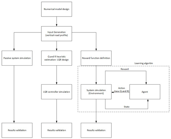
Figure 1.
Scheme of conducted experiments.
In the next step, extortion in accordance with the standard in [31] was introduced. This standard refers to unifying vertical profile data for roads, streets, highways and off-road profiles. It uniquely defines the ground vertical profile data. From there, it was used to generate a standardised input in the form of an assumed road profile, which became the input signal for the numerical model. Such a system generated the response for each state variable for the passive solution and the classical LQR controller. In the case of a neural network, a design in which a reward function is present was applied. This function is explained in more detail in Section 2.2. This approach aims to replace the relatively laborious and challenging process of selecting the parameters of the Q and R matrices by introducing an intuitive mechanism for rewarding the agent for the modifications applied to the values of these matrices. Based on its previous actions, the current action and the effects of the agent’s actions on the system under study, subsequent modifications are made to the Q and R matrix coefficients. The modification of the parameters occurs after the entire road is generated according to the ISO standard, so one epoch of learning the agent (iterative calculation of new Q and R parameters) was performed not point by point but after passing the entire generated road profile. Learning is terminated when the required control quality is achieved. In order to evaluate each type of control, the control evaluation indicators included in Section 3 are proposed.
2.1. Mathematical Modeling
A mathematical model with lumped parameters of a quarter suspension of a wheeled vehicle (Figure 2) was subjected to simulation analysis. This model corresponds to one strut of the vehicle’s suspension. It consists of a sprung mass , which represents the chassis part per suspension strut, and an unsprung mass , which represents the moving elements of the suspension, such as the tire, including the rim, the swing arm and the steering knuckle. The tire is represented as a spring element . The tire viscous damping was omitted due to its negligible effect on the dynamics of the whole model. The vehicle suspension components were modelled as a spring element and a viscous damping element . In the case of an active suspension system, the important element is the actuator, which can be a hydraulic actuator or another actuator with linear motion, such as an electric actuator. The force generated by the actuator is denoted as . Displacements in the vertical direction of the sprung mass and unsprung mass are denoted as and , respectively. The presented model reduces the complex motion of the suspension components to linear motion and has been widely used in the literature [32,33,34,35,36]. The model does not include an additional degree of freedom representing the driver’s seat, assuming that minimising the vibration of the entire body improves travel comfort. The model parameters were determined from [32] and are presented in Table 1.
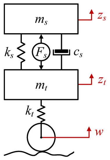
Figure 2.
Model of the active suspension strut.

Table 1.
Model parameters.
The model was described by a system of two second-order differential equations that include the equilibrium force equations for each mass (1) and (2) [32,37]. The model was described at the static equilibrium point of the system, where the gravity force is balanced by the static deflection of the suspension spring and tire. Therefore, the gravity force has yet to be included explicitly in the equations describing the system.
A representation of the active suspension strut model in the state space is given by the following Equations (3)–(5):
The input matrix B of the system was decomposed into a matrix of controllable input, , related to the force generated by the actuator and non-controllable input, , related to the kinematic excitation, w, from the road irregularity. We may consider the uncontrollable input w as a disturbance acting on our object. The controllability and stability conditions have been fulfilled.
The aim of the control is to keep the system in equilibrium or at a preset operating point, despite the disturbances acting on it. This task involves determining the control that minimises the standard squared performance index:
by determining the matrix K of the control signal, is then given by the relation:
The matrix K is the gain matrix of the state variables uniquely determined by the LQR method [3,6,9]. Then, a closed-loop system with feedback from state variables to controllable input is then described by a state equation:
and the output of Equation (4).
The coefficients of the diagonal matrix Q result from assuming the performance index as a weighted arithmetic mean of the indicators corresponding to each vehicle suspension’s evaluation criteria, such as comfort, safety (grip) and ground clearance (suspension travel). The R coefficient was selected to ensure that the system operates within the relevant range of control signals [38].
2.2. Neural Model Architecture
The primary purpose of the neural algorithm is to obtain Q and R matrices for calculating the gain matrix K by the LQR algorithm. In order to achieve such functionality, the Reinforcement Learning (RL) algorithm was modified. A relatively simple DQN agent with continuous observation and discrete action space was used. Since the goal was not to obtain an agent with a specific behaviour but a specific one-time response, the choice of agent is of secondary importance. The system’s architecture is shown in Figure 3. The entire learning algorithm is based on taking action through an agent.
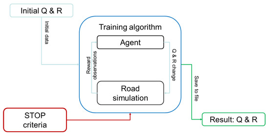
Figure 3.
The architecture of the system for selecting quality matrix settings Q and resources R.
2.2.1. Observation Vector
The environment provides the agent with a vector of observations consisting of the results of a simulated road trip and the current parameters (or initial parameters for the first iteration) of the matrices Q and R. The observation vector includes the following constant vectors (C) and modified vectors (M):
- –
- —sprung mass (C);
- –
- —unsprung mass (C);
- –
- —suspension spring stiffness coefficient (C);
- –
- —stiffness coefficient of tyre (C);
- –
- —suspension viscous damping coefficient (C);
- –
- Q—quality matrix (M);
- –
- R—resources matrix (M).
Constant vectors were introduced because adaptability to nonlinear system parameters will be tested in future studies. In contrast, the agent modifies the parameters of the Q and R matrices in each iteration.
2.2.2. Reward Function
Based on the observations of the system state, the agent decides on the following action. As shown in the [27], it is impossible to fully understand the sequence of actions performed from the current observation. Therefore, the agent remembers previous states and the impact of subsequent actions taken on the reward. Therefore, the agent analyses the subsequent actions and observations sequence and, based on this, learns the strategies for changing the matrices Q and R. All the agent’s actions are carried out in such a way so as to maximise the reward function. This is a crucial element of the method, as it leads to obtaining the assumed quality of control by intuitively determining the critical parameters for the user. The reward function is defined by the relations (9)–(14):
where
- –
- —standard deviation of the force generated by the actuator;
- –
- —standard deviation of the dynamic component of the wheel load force on the ground;
- –
- —static component of the contact force;
- –
- —standard deviation of the sprung mass displacement;
- –
- —penalty for exceeding the forces realisable by the actuator according to the three-sigma rule;
- –
- —penalty for exceeding the dynamic component of the wheel load force according to the three-sigma rule;
- –
- —reward for reducing the standard deviation of the sprung mass displacement to a level below 0.005 m;
- –
- —reward for reducing the standard deviation of the sprung mass displacement to a level below 0.004 m;
- –
- —penalty for errors in creating the LQR;
- –
- —reward.
Taking an analytical approach to the penalty function, the actor receives the smallest penalty in the case of and . In the first case, the system is penalised when the control developed based on the matrix coefficients selected by the system is not realisable by the actuator. According to the three-sigma rule, such a situation occurs when three times the standard deviation of the active force exceeds the maximum force that the actuator can provide. In the second case, the wheel is detached from the ground (according to the three-sigma rule with a probability of 99.7%) when three times the standard deviation of the dynamic component of the load force, , exceeds the static load force, . It is an unacceptable situation leading to a loss of traction; therefore, a safety factor of 0.75 was assumed. The actor will already be penalised 25% before the developed control allows the wheel to detach from the roadway. It is a penalty that affects the driving safety rating. The and penalties are related to the user’s sense of comfort. They are positive, so the actor is rewarded for providing adequate comfort for the person being transported. Note that the system designer selected an penalty more than an order larger than the previous two penalties because it was considered that user comfort is a significant component of the system’s performance assessment. In addition, if the actor finds values for the parameters of the quality matrix, Q, and the resources matrix, R, that further reduce the standard deviation of the vehicle’s body displacement. The reward is two orders higher than the reward . The penalty is due to the assumption that the obtained coefficients of the matrix should make it positive definite so that stable operation of the LQR controller can be obtained. It is dictated by the requirements of a correct operation of the control system. The aggregate reward function also takes into account the standard deviation, , of the vehicle body displacement directly. The larger it is, the more the agent is penalised.
2.2.3. Agent Definition
The agent’s action space is discrete. It is necessary to force small (on the order of ) steps in the space of possible Q and R. Action space was provided by generating a matrix of all combinations of the vector . The agent can move through Q and R space with only such discrete steps. It allows for small and large values of Q and R in a single learning episode. In order to force an agent’s specific behaviour, the value of R is multiplied by , which increases the possible forces applied by the LQR controller.
2.2.4. Training Algorithm
Each learning step begins by loading the stored values from the previous step (or initial values), and then the action taken by the agent is transformed into the change value of Q and R, which is summed with the loaded values. The positivity condition of the Q and R matrices is then checked, ensuring that the LQR controller can be formed and is stable. If any of the matrices are not positive definite, the environment generates a penalty and skips the simulation run. If the matrices meet the conditions, the environment generates the LQR and loads the road data for simulation. The simulation of driving the specified road is then carried out, and the measurement results are passed on to calculate the reward value. The reward is calculated based on the standard deviation of the value (multiplied by ). In addition, an additional penalty was added for exceeding permissible forces and permissible tire deflection. Then the condition for writing Q and R was checked. If it was met, the values were written to the file, and the agent received a reward. A single learning cycle consisted of 2000 episodes of up to 250 steps each. At the end of the learning cycle, the stored Q and R values were compared in terms of extended integral indicators of control quality and the best one was selected. The functional diagram is shown in Figure 4.
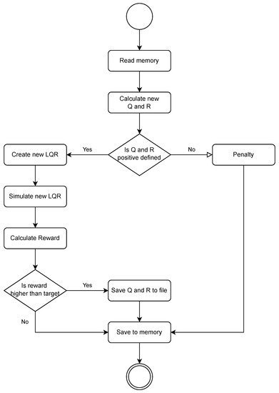
Figure 4.
Diagram of a single learning step.
3. Results
In the classic approach to designing a linear quadratic controller, the values of matrix coefficients Q and R are iteratively selected by the designer so that the control system meets the assumed requirements and physical constraints of the actuators. This paper presents a method of selecting the Q and R matrix elements using a neural network. Such an approach relieves the designer from selecting specific numerical values of the elements of the weight matrices, instead expecting them to specify the desired comfort level and safety of the active suspension strut at the stage of creating the neural network reward function. For the system with a classic Linear Quadratic Regulator (LQR system), the form of the diagonal Q matrix and R coefficient are adopted according to (15), while for the system supported by a neural network (NN LQR system), the matrix and coefficient are adopted according to (16).
One of the basic criteria for evaluating vibroisolation systems is the vibration transmissibility ratio. This ratio is considered in the frequency domain and can be defined as a displacement transmissibility function. In order to assess comfort, the displacement transmissibility function, , described by the relation (17) was adopted. Non-logarithmic displacement transmissibility functions, T, are defined as the ratio of modulus from the Fourier transform of the selected input and output signals (). This function illustrates how the kinematic excitation from the road irregularity affects the vertical displacement of the sprung mass. For linear objects, this function is the modulus of the spectral transfer function of the object from input w to output . The displacement function of the tire deflection, , given by the relation (18) was used to evaluate the safety. This function illustrates how the kinematic excitation from road irregularity affects the dynamic deformation of the tire. In the case of both functions, smaller values of the function mean better suspension performance in a given aspect. The function given by Equation (19) is a function of the force generated by the actuator in the frequency domain.
The obtained frequency characteristics are shown in Figure 5. For active suspension systems, the function takes values less than zero for the entire analysed frequency range. It can be seen that the vehicle’s active suspension systems improve travel comfort in almost the entire analysed frequency range, especially in the low frequency range. The ability to reduce vibrations at low frequencies is one of the main advantages of using active vibration reduction systems over passive vehicle suspension systems. It is worth noting that the NN LQR system reduces both the values of the functions and in the neighbourhood of the higher resonant frequency compared to the LQR system. In addition, for excitations in the frequency range from 1 to 6 Hz, the NN LQR system has the highest comfort among the analysed systems.
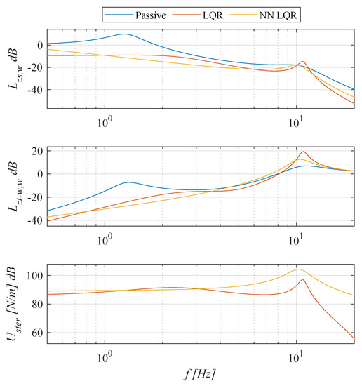
Figure 5.
Comparison of the frequency characteristics of the analysed systems.
Moreover, frequency domain integral performance indexes are given by Equation (20) and were introduced to evaluate the suspension.
These performance indexes correspond to the average value of a given vibration transmissibility function in the analysed frequency range from start frequency Hz to final frequency Hz. The performance index determines the comfort level of a given suspension strut; smaller values of the performance index mean a smaller average displacement of the sprung mass and thus a higher level of comfort provided by a given suspension system. Similarly, the performance index determines the safety level of a given suspension strut; smaller values of the performance index mean smaller average dynamic deformation of the vehicle’s tire and therefore a higher level of safety provided by a given suspension.
A comparison of the calculated performance indexes is shown in Figure 6. It can be seen that there is a significant improvement in comfort for both active systems compared to the passive suspension strut. The indexes representing safety in the case of the active systems, although taking higher values than the passive system, are acceptable for harmonic excitations. The NN LQR system achieves better performance indexes than the LQR system in terms of comfort and safety.
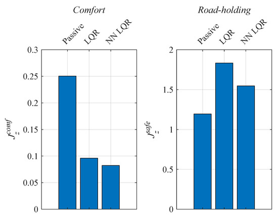
Figure 6.
Comparison of performance indexes of the analysed suspension systems.
A random signal of excitation due to road irregularities generated in accordance with [31], simulating the passage of a tested suspension strut through a road in different quality classes at a constant speed of 60 km/h, was used to determine the time domain performance indexes. The standard defines the basic stochastic parameters of acceptable inequalities for different road classes. The road quality defined by the standard is described by a given distribution of the power spectral density of the road irregularities as a function of the angular spatial frequency. The applied kinematic excitation due to road irregularities is shown in Figure 7. The generator of used random excitation is described in [39,40]. Each simulation lasted at least 100 s. Simulations were carried out for excitations conforming to road classes A-B, B-C and C-D [41].
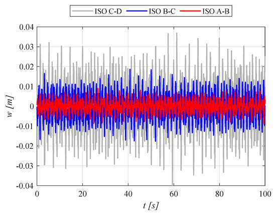
Figure 7.
Time courses of excitation due to road irregularities generated according to [31] at a constant driving speed of 60 km/h.
Sample results of the simulation tests are presented in Figure 8. The figure shows only the first 10 s of the 100 s simulation time for illustrative purposes. There is zero mean value of excitation and model response for the entire simulation time. It can be seen that there is a significant improvement in comfort by both active suspension systems compared to passive suspension. The displacements of the sprung mass were reduced by the LQR and NN LQR active systems compared to the passive system. The tire dynamic deformation, , remains at an acceptable level.
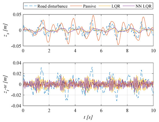
Figure 8.
Time courses of sprung mass displacement and tire deflection (ISO C-D, 60 km/h).
The time courses of the force generated by the actuator are shown in Figure 9. The maximum force values do not exceed the assumed performance of the actuator system. For the LQR system, this was the main factor in the iterative selection of the value of the coefficient R. For the NN LQR system, the maximum force values that the actuator can provide were taken directly into account in the neural network’s reward function, and exceeding them involved a significant penalty for the neural network.
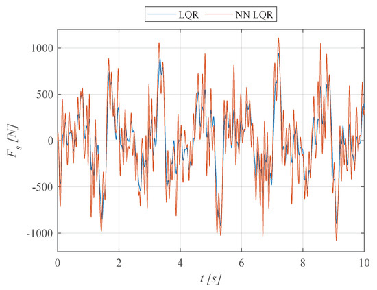
Figure 9.
Time courses of the force generated by the actuator (ISO C-D, 60 km/h).
A comparison of the calculated suspension time domain performance indexes is shown in Table 2. The table summarises the suspension system quality evaluation indicators regarding standard deviations of specific displacements or forces. The value indicates the standard deviation of the excitation displacement from the road’s unevenness.
Table 2.
Comparison of suspension time domain performance indexes.
The following suspension time domain performance indexes were adopted:
- –
- —standard deviation of the sprung mass displacement, comfort rating;
- –
- —standard deviation of dynamic tire deformation, safety assessment;
- –
- —standard deviation of the dynamic component of the wheel load force on the ground, safety assessment;
- –
- —standard deviation of the force generated by the actuator, evaluation of the realisability of the algorithm by the actuator unit.
It is apparent that there is a significant improvement in ride comfort for active suspension systems regardless of the simulated road category. In the case of active suspension systems, the standard deviation of the sprung mass is approximately five times smaller than in a passive one in all simulated cases. The differences between the LQR and NN LQR systems in terms of comfort are minor, at around 10%. The forces generated by the actuator in the NN LQR system are slightly larger than those of the LQR system, but they are realisable by the actuator. The tire’s dynamic deformation standard deviation for the NN LQR system is about 2% smaller than the LQR system. The NN LQR system has better safety rating indicators while maintaining equally good comfort rating indicators compared to the LQR system.
In terms of driving safety, the ability of a vehicle’s suspension to maintain wheel contact with the ground plays a key role. The tangential forces that provide traction and vehicle handling are closely related to the wheel-to-ground forces. In order to better assess driving safety, an additional quality assessment index was introduced:
which is the dynamic component of the wheel–ground contact force. According to [42], in order to ensure safety, it is necessary to minimise the ratio of the dynamic component of the contact force, , to the static component of the contact force, :
In the presented system, the static load is 4415 N. The static load was calculated as the pressure of the suspension system on the ground in static equilibrium. Therefore, it is the sum of the sprung and unsprung masses multiplied by the gravitational acceleration with parameters according to Table 1 according to the formula:
A high dynamic component of the contact force leads to loss of grip. In the reward function of the neural network, the critical and non-exceedable value is the inequality:
taking into account the additionally adopted safety factor of 0.75.
Thus, the NN LQR system met the adopted assumptions. The LQR system is characterised by a larger performance index than the NN LQR system. Despite this, even for the C-D road class, it met the criterion ; however, without the assumed safety factor of 0.75.
4. Conclusions
A vehicle’s suspension can be excited to oscillate by surface irregularities on a road. In order to prevent such a phenomenon and to improve stability, a system with an LQR controller is proposed, in which the coefficients of the Q and R matrices are selected using a neural reasoning system. The presented research focuses on finding the most optimal settings possible by simulating vehicle oscillations for a quarter-dynamics model with forcing from the road surface. The proposed solution is compared with a passive system and an LQR controller with heuristically selected parameters. The design process of the neural optimiser is shown. According to the simulation results, the displacement and acceleration values of the protected mass were improved, and user comfort increased compared to the passive and heuristic LQR control.
This article shows how to solve the posed problem using the DQN algorithm. The results presented allow us to identify the main advantages of the method:
- –
- The algorithm allows intuitive influence on the quality of the target control. By determining the penalty function, the DQN network in probabilistic space adjusts the values of the parameters of the matrices Q and R to those that realise the assumed quality of control with the LQR controller;
- –
- The algorithm allowed a 67% improvement in user comfort over the passive solution and a 14% improvement over the LQR controller with parameters selected by an expert with 20 years of experience in controlling suspension systems;
- –
- At the same time, better road holding performance was achieved relative to the standard LQR with a significant reduction in impact forces.
In classical and renewable energy, multidimensional actuators related to energy conversion dominate. In most cases, they are not optimally controlled, and control quality can be improved even if an LQR controller is used. Unfortunately, due to both the parametric uncertainty of the model and the lack of sufficient expertise, most often, measures to improve this quality still need to be taken. The proposed solution with neural tuning of the quality matrix, Q, and resources matrix, R, is scalable and can also be used for such systems. The basis is the determination of the penalty function, which will allow us to intuitively guide the DQN network to such learning that will achieve the assumed control quality for each state variable important to the designer. An additional advantage of the proposed method is that it can be used for nonlinear systems often encountered in power conversion systems. In this case, for different operating points, it is necessary to linearise the object model, and then the network develops sets of parameters of the Q and R matrices that will lead to high control quality in each of the linearised models. This issue will be the subject of further research work.
Author Contributions
Conceptualization, M.K. and A.S.; methodology, M.K. and A.S.; software, M.K. and A.S.; validation, M.K., A.S. and K.L.; formal analysis, A.S.; investigation, M.K.; resources, M.K. and A.S.; data curation, M.K.; writing—original draft preparation, M.K., A.S. and K.L.; writing—review and editing, M.K., A.S. and K.L.; visualization, A.S.; supervision, K.L.; project administration, K.L.; funding acquisition, M.K. All authors have read and agreed to the published version of the manuscript.
Funding
This research was funded by AGH University of Science and Technology research subsidy number 16.16.130.942.
Data Availability Statement
Not applicable.
Conflicts of Interest
The authors declare no conflict of interest. The funding sponsors had no role in the design of the study; in the collection, analyses, or interpretation of data; in the writing of the manuscript; or in the decision to publish the results.
Abbreviations
The following abbreviations are used in this manuscript:
| LQR | Linear Quadratic Regulator |
| RL | Reinforcement Learning |
| DQN | Deep Q-Network |
| MIMO | Multi-Input Multi-Output |
| SISO | Single-Input Single-Output |
| PSO | Particle Swarm Optimization |
| PI | Proportional Inertial |
| LQG | Linear Quadratic Gaussian |
References
- Radaideh, A.; Bodoor, M.; Al-Quraan, A. Active and Reactive Power Control for Wind Turbines Based DFIG Using LQR Controller with Optimal Gain-Scheduling. J. Electr. Comput. Eng. 2021, 2021, 1218236. [Google Scholar] [CrossRef]
- Elia, N.; Mitter, S.K. Stabilization of linear systems with limited information. IEEE Trans. Autom. Control 2001, 46, 1384–1400. [Google Scholar] [CrossRef]
- Goodwin, G.C.; Graebe, S.F.; Salgado, M.E. Control System Design; Prentice Hall: Upper Saddle River, NJ, USA, 2001; Volume 240. [Google Scholar]
- Zhang, R.; Li, Y.; Li, N. On the regret analysis of online LQR control with predictions. In Proceedings of the 2021 American Control Conference (ACC), New Orleans, LA, USA, 25–28 May 2021; pp. 697–703. [Google Scholar]
- Simon, D. Optimal State Estimation: Kalman, H∞, and Nonlinear Approaches; John Wiley & Sons, Ltd.: Hoboken, NJ, USA, 2006. [Google Scholar] [CrossRef]
- Ogata, K. Modern Control Engineering; Prentice Hall: Upper Saddle River, NJ, USA, 2010; Volume 5. [Google Scholar]
- Song, J.; Chen, W.; Guo, S.; Yan, D. LQR control on multimode vortex-induced vibration of flexible riser undergoing shear flow. Mar. Struct. 2021, 79, 103047. [Google Scholar] [CrossRef]
- Johansen, T.A.; Petersen, I.; Kalkkuhl, J.; Ludemann, J. Gain-scheduled wheel slip control in automotive brake systems. IEEE Trans. Control Syst. Technol. 2003, 11, 799–811. [Google Scholar] [CrossRef]
- Åström, K.J.; Wittenmark, B. Adaptive Control; Courier Corporation: Chelmsford, UK, 2013. [Google Scholar]
- Lu, Y.; Khajepour, A.; Soltani, A.; Li, R.; Zhen, R.; Liu, Y.; Wang, M. Gain-adaptive Skyhook-LQR: A coordinated controller for improving truck cabin dynamics. Control Eng. Pract. 2023, 130, 105365. [Google Scholar] [CrossRef]
- Narayan, J.; Dwivedy, S.K. Robust LQR-based neural-fuzzy tracking control for a lower limb exoskeleton system with parametric uncertainties and external disturbances. Appl. Bionics Biomech. 2021, 2021, 5573041. [Google Scholar] [CrossRef]
- Abdullah, H.N. An improvement in LQR controller design based on modified chaotic particle swarm optimization and model order reduction. Int. J. Intell. Eng. Syst. 2021, 14, 157–168. [Google Scholar] [CrossRef]
- Peng, G.; Chen, C.P.; Yang, C. Neural networks enhanced optimal admittance control of robot-environment interaction using reinforcement learning. IEEE Trans. Neural Netw. Learn. Syst. 2021, 33, 4551–4561. [Google Scholar] [CrossRef]
- Grondman, I.; Buşoniu, L.; Babuška, R. Model learning actor-critic algorithms: Performance evaluation in a motion control task. In Proceedings of the 2012 IEEE 51st IEEE Conference on Decision and Control (CDC), Maui, HI, USA, 10–13 December 2012; pp. 5272–5277. [Google Scholar]
- Nguyen, M.L.; Tran, T.T.H.; Nguyen, T.A.; Nguyen, D.N.; Dang, N.D. Application of MIMO Control Algorithm for Active Suspension System: A New Model with 5 State Variables. Lat. Am. J. Solids Struct. 2022, 19. [Google Scholar] [CrossRef]
- Pillai, A.G.; Rita Samuel, E. PSO based LQR-PID output feedback for load frequency control of reduced power system model using balanced truncation. Int. Trans. Electr. Energy Syst. 2021, 31, e13012. [Google Scholar] [CrossRef]
- Murari, A.; Rodrigues, L.; Altuna, J.; Potts, A.S.; Almeida, L.; Sguarezi Filho, A. A LQRI power control for DFIG tuned by a weighted-PSO. Control Eng. Pract. 2019, 85, 41–49. [Google Scholar] [CrossRef]
- Jeon, T.; Paek, I. Design and verification of the LQR controller based on fuzzy logic for large wind turbine. Energies 2021, 14, 230. [Google Scholar] [CrossRef]
- Dominik, I. Implementation of the type-2 fuzzy controller in PLC. Solid State Phenom. 2010, 164, 95–98. [Google Scholar] [CrossRef]
- Dominik, I. Interval type-2 fuzzy logic control of DM series shape memory actuator. Solid State Phenom. 2014, 208, 116–124. [Google Scholar] [CrossRef]
- Samad, B.A.; Mohamed, M.; Anavi, F.; Melikhov, Y. A hybrid Fuzzy approach of different controllers to stabilize a 3-link swinging robotic (Robogymnast). In Proceedings of the 2022 2nd International Conference on Advance Computing and Innovative Technologies in Engineering (ICACITE), Greater Noida, India, 28–29 April 2022; pp. 2432–2437. [Google Scholar]
- Bekkar, B.; Ferkous, K. Design of Online Fuzzy Tuning LQR Controller Applied to Rotary Single Inverted Pendulum: Experimental Validation. Arab. J. Sci. Eng. 2022, 1–16. [Google Scholar] [CrossRef]
- Lu, E.; Yang, X.; Li, W.; Wang, Y.; Fan, M.; Liu, Y. Tip position control of single flexible manipulators based on LQR with the Mamdani model. J. Vibroeng. 2016, 18, 3695–3708. [Google Scholar] [CrossRef]
- Meng, Q.X.; Lai, X.Z.; Wang, Y.W.; Wu, M. A fast stable control strategy based on system energy for a planar single-link flexible manipulator. Nonlinear Dyn. 2018, 94, 615–626. [Google Scholar] [CrossRef]
- Wahid, N.; Rahmat, M.F. Pitch control system using LQR and Fuzzy Logic Controller. In Proceedings of the 2010 IEEE Symposium on Industrial Electronics and Applications (ISIEA), Tehran, Iran, 17–18 February 2010; pp. 389–394. [Google Scholar]
- Hazem, Z.B.; Fotuhi, M.J.; Bingül, Z. Development of a Fuzzy-LQR and Fuzzy-LQG stability control for a double link rotary inverted pendulum. J. Frankl. Inst. 2020, 357, 10529–10556. [Google Scholar] [CrossRef]
- Rahman, M.; Rashid, S.; Hossain, M. Implementation of Q learning and deep Q network for controlling a self balancing robot model. Robot. Biomimetics 2018, 5, 8. [Google Scholar] [CrossRef]
- Lu, F.; Mehta, P.G.; Meyn, S.P.; Neu, G. Convex Q-learning. In Proceedings of the 2021 American Control Conference (ACC), New Orleans, LA, USA, 25–28 May 2021; pp. 4749–4756. [Google Scholar]
- Poznyak, A.S.; Sanchez, E.N.; Yu, W. Differential Neural Networks for Robust Nonlinear Control: Identification, State Estimation and Trajectory Tracking; World Scientific: Singapore, 2001. [Google Scholar]
- Caarls, W. Deep Reinforcement Learning with Embedded LQR Controllers. IFAC-PapersOnLine 2020, 53, 8063–8069. [Google Scholar] [CrossRef]
- Mechanical Vibration–Road Surface Profiles–Reporting of Measured Data; International Organization for Standardization: Geneva, Switzerland, 1995; Volume 8608.
- Savaresi, S.M.; Poussot-Vassal, C.; Spelta, C.; Sename, O.; Dugard, L. Semi-Active Suspension Control Design for Vehicles; Elsevier: New York, NY, USA, 2010. [Google Scholar]
- Rajamani, R. Vehicle Dynamics and Control; Springer: New York, NY, USA, 2012. [Google Scholar] [CrossRef]
- Konieczny, J. Modelling of the electrohydraulic full active vehicle suspension. Eng. Trans. 2008, 56, 247–268. [Google Scholar]
- Popp, K.; Schiehlen, W. Ground Vehicle Dynamics; Springer Science & Business Media: Berlin/Heidelberg, Germany, 2010. [Google Scholar]
- Wong, J.Y. Theory of Ground Vehicles; John Wiley & Sons: New York, NY, USA, 2022. [Google Scholar]
- Ogata, K. System Dynamics; Pearson Education Limited: Auckland, New Zealand, 2013. [Google Scholar]
- Smoter, A.; Sibielak, M. Experimental and numerical investigation of the active double wishbone suspension system. In Proceedings of the 2019 20th International Carpathian Control Conference (ICCC), Krakow-Wieliczka, Poland, 26–29 May 2019; pp. 1–6. [Google Scholar]
- Konieczny, J.; Sibielak, M.; Rączka, W. The Control System for a Vibration Exciter. Solid State Phenom. 2013, 198, 600–605. [Google Scholar] [CrossRef]
- Konieczny, J.; Kowal, J.; Sapiñski, B. Synthesis of a mechanical oscillator as a source of disturbances for active vibration reduction systems. In INTER-NOISE and NOISE-CON Congress and Conference Proceedings; Institute of Noise Control Engineering: Reston, VA, USA, 1999; Volumes 1–2, pp. 137–144. [Google Scholar]
- Priyambodo, T.K.; Dhewa, O.A.; Susanto, T. Model of Linear Quadratic Regulator (LQR) Control System in Waypoint Flight Mission of Flying Wing UAV. J. Telecommun. Electron. Comput. Eng. 2020, 12, 43–49. [Google Scholar]
- Mitschke, M.; Wallentowitz, H. Beurteilungsmaßstäbe und ihre Berechnung. In Dynamik der Kraftfahrzeuge; Springer: Wiesbaden, Germany, 2014; pp. 349–367. [Google Scholar]


Disclaimer/Publisher’s Note: The statements, opinions and data contained in all publications are solely those of the individual author(s) and contributor(s) and not of MDPI and/or the editor(s). MDPI and/or the editor(s) disclaim responsibility for any injury to people or property resulting from any ideas, methods, instructions or products referred to in the content. |
© 2023 by the authors. Licensee MDPI, Basel, Switzerland. This article is an open access article distributed under the terms and conditions of the Creative Commons Attribution (CC BY) license (https://creativecommons.org/licenses/by/4.0/).