Electrical Load Forecasting Using LSTM, GRU, and RNN Algorithms

Abstract

Forecasting the electrical load is essential in power system design and growth. It is critical from both a technical and a financial standpoint as it improves the power system performance, reliability, safety, and stability as well as lowers operating costs. The main aim of this paper is to make forecasting models to accurately estimate the electrical load based on the measurements of current electrical loads of the electricity company. The importance of having forecasting models is in predicting the future electrical loads, which will lead to reducing costs and resources, as well as better electric load distribution for electric companies. In this paper, deep learning algorithms are used to forecast the electrical loads; namely: (1) Long Short-Term Memory (LSTM), (2) Gated Recurrent Units (GRU), and (3) Recurrent Neural Networks (RNN). The models were tested, and the GRU model achieved the best performance in terms of accuracy and the lowest error. Results show that the GRU model achieved an R-squared of 90.228%, Mean Square Error (MSE) of 0.00215, and Mean Absolute Error (MAE) of 0.03266.

1. Introduction

The last era in the world was generally characterized by the rapid and large expansion of electricity networks, especially electrical loads, as they swelled dramatically and new types of these electrical loads appeared that need a special study [1]. The increase in electrical loads causes complexity in the design of the electrical system components. The reorganization of the energy system also led to the formation of institutionalized generation, transmission, and distribution companies. These entities are challenged by the increasing requirements for the reliable operation of power system networks [2]. The main concern of every electrical company is to provide reliable and continuous service to its customers. It has become difficult to predict electrical loads using traditional and old methods since many factors affect electrical loads directly and indirectly. Those factors are population census, temperatures, climatic changes, rainwater, underground basins, the economic system in each country, human behavior, global epidemics, and the evolution of industries [3]. Electricity in Palestine is taken from the Israeli through connection points between the two sides, and some of these points have high electricity consumption and others low consumption, which causes malfunctions in high-load transformers and leads to problems in energy outputs and infrastructure. Electrical load forecasting is critical in establishing and improving power system efficiency because it ensures reliable and economic planning, control, and operation of the power system. It helps the electricity companies make critical choices such as the acquisition and generation of electrical power, as well as the establishment of the infrastructure for the transmission and distribution system.

With the rapid and dramatic increase in energy consumption, developing reliable models to predict electrical loads is becoming increasingly demanded and complicated [4,5]. The problem of rapid and sharp growth in energy consumption in Palestine has led to the need to create reliable models to predict electricity loads, as these models will help the electricity companies in managing and planning energy transmission and ensuring reliable and uninterrupted service to their customers. Predicting electrical loads is very important for electricity companies in Palestine to prepare short, medium, and long-term plans, and the energy authority and government agencies need to secure energy in the coming years.

Forecasting the electrical loads does not depend only on the power sector in Palestine, but instead can feed all economic sectors for feedback that may benefit them in preparing plans for future development for these sectors. Globally, the importance of predicting loads comes from the difficulty of predicting them, as loads are the missing and most ambiguous link for many countries that seek to develop strategies for the electrical system. Therefore, load forecasting is useful in t designing electrical networks and developing strategic plans that ensure a stronger economy, a cleaner environment, and energy sustainability.

In this research, we are going to forecast the short-term electrical loads in Palestine based on real data and deep learning algorithms namely: long short-term memory (LSTM), gated recurrent unit (GRU), and recurrent neural network (RNN). The objectives of this work can be illustrated as follows:

• Forecasting electrical loads with the highest accuracy to simulate the real development of electrical loads.
• Assisting electrical companies in developing short and medium-term plans for designing electrical networks and estimating infrastructure needs.
• Improving the electricity service in Palestine and solving the problem of power outages in Palestine.
• Helping the electricity companies in securing sources of energy that are suitable for the loads and not reduce the loads; as this increase is considered a waste that cannot be used.

The main contribution of this study is to develop models using deep learning algorithms (RNN, LSTM, and GRU) to forecast electricity load in Palestine based on a novel real dataset. This dataset is the first to come to light in a specific area (Palestine). In addition to the tuning that was performed using different types of Hyperparameters (optimizer, activation function, learning rate, number of epochs, batch size, number of hidden layers, and dropout). To the best of the authors knowledge there is no studies in the open literature review conducted to forecast the electrical loads using seven types of Hyperparameters. The proposed forecasting models presented in this research can be applied to any electricity company dataset. The forecasting models will help electricity companies to introduce reliable and uninterrupted services to their customers, assist them in developing short and medium-term plans for designing electrical networks and estimating infrastructure needs, and help them in securing sources of energy that are suitable for the loads. Moreover, the proposed models will help the electric companies to make critical decisions, such as the development of transmission and distribution systems infrastructure to guarantee the best electrical services for the customers.

This section provides an overview of the electrical load forecasting and the following sections in the paper are structured as follows: Section 2 describes the literature review and previous studies, Section 3 presents the methodology used in building the deep learning models to forecast the electric load, Section 4 illustrates the experimental results and compares the results with previous studies. Section 5 provides conclusions and plan for future work.

2. Literature Review

This section presents the state of the arts and an analysis of the relevant literature review for the forecasting of electrical loads and demands.

2.1. Background

Machine learning (ML) and deep learning algorithms are widely used in the field of forecasting energy demand and the amount of electricity consumption [6]. Engineers and data scientists depend on these approaches to deal with temporal data in terms of exploration, explanation, and analysis. Deep learning algorithms are used to optimally manage the competitive markets of electricity, heat, and hydrogen by tapping into the potential of intelligent consumers. Through using the capabilities of data-driven customers, deep learning algorithms are employed to efficiently control the dynamic electricity, heat, and hydrogen markets [7]. At a high level, the use of ML in power demand analysis in the literature is separated into two types and those are: (1) unsupervised learning techniques, which are primarily used to give descriptive analytics or as pre-processing stages and discover the behavior of electricity consumption [8,9,10,11], and (2) supervised learning approaches, which are mostly used for predictive modeling [12,13,14,15,16].

One of the most obstacles that face the Palestinian electricity companies is forecasting the electricity loads since the forecasting process helps these companies guarantee the electrical services to their customers, reduce power outages, and management of their electrical network, so there is a need for building a reliable electricity load forecasting system to predict future power loads in Palestine. It is worth mentioning that we cannot depend on the power loads forecasting system that had been proposed in the literature by the previous researchers since the weather factors and the power sources differ from country to country.

2.2. Electrical Load Forecasting

Load forecasting can be loosely classed as engineering techniques or information methodologies techniques. Engineering techniques, often defined as physics-based modeling, employ physical rules to forecast and evaluate power consumption. To compute energy use, these models frequently rely on contextual elements such as the structure of the building, meteorology, and heated, ventilated, heating, and cooling information. In addition, many mathematical operations and equations are needed for prediction purposes. Building energy simulator tools such as energy plus and equest use physics-based models [17]. The limitations of these models originate from their reliance on the accessibility and accuracy of the training dataset [18]. Researchers proposed two sorts of forecasting techniques: quantitative and qualitative [19,20]. Quantitative approaches include moving averages [21], deep learning methods [22], time series [23], exponential smoothing [24], and trend projection [25]. They are employed when the situation is steady and previous data is available. Whereas, qualitative procedures [26] such as Delphi methodologies [27] and high-level experts [28] are employed when the situation is ambiguous and there is limited available data.

2.3. Short-Term Load Forecasting (STLF)

STLF is essential to lower the cost of electricity transactions, encourage the reliable functioning of smart grids without interruption, and control loads as needed. STLF is also used to assess the risks of electricity shortages and reduce the appearance of loads to obtain a stable and reliable electrical network. This section will talk about the following subsections: short-term load forecasting for medium and large electrical networks, and short-term load forecasting for small electrical networks.

2.3.1. Short-Term Load Forecasting for Medium and Large Electrical Networks

The models proposed in [29] is based on neural networks and particle swarm optimization (PSO) to evaluate the Iranian power system. The neural network-based solutions resulted in fewer prediction mistakes due to their capacity to adapt effectively the hidden properties of the consuming load. The accuracy of the proposed model was assessed based on the mean absolute percentage error (MAPE) which does not exceed 0.0338 and the mean absolute error (MAE) was found to be 0.02191.

The studies in [30,31] used empirical modal decomposition (EMD), where it makes the original electricity consumption data is first decomposed into several inherent mode functions (IMFS) with different frequencies and amplitudes. Researchers in [30] suggested empirical mode decomposition gated recurrent units with feature selection for short-term load forecasting (EMD-GRU-FS). The Pearson correlation is used as the prediction model’s input feature to determine the correlation between the subseries and the original series. The experimental findings revealed that the suggested method’s average prediction accuracy on four data sets was 96.9%, 95.31%, 95.72%, and 97.17%, consecutively. Moreover, authors in [31] enhanced a combination of integrated empirical modal decomposition (EMD) and long short-term memory network (LSTM) was presented for short-term load power consumption forecasting. The LSTM is used to extract features and make temporal predictions. Finally, on the end-user side, short-term electricity consumption prediction results were obtained by accumulating multiple target prediction results. The proposed EMD—LSTM method achieved MAPE of 2.6249% in the winter and 2.3047% in the summer.

Moreover, in China, a hybrid short-load forecasting system based on variation mode decomposition (VMD) and long short-term memory (LSTM) networks and optimized using the Bayesian optimization algorithm (BOA) has been developed [32]. They compared the proposed methods with SVR, multi-layered perceptron regression, LR, RF, and EMD-LSTM, the result of the proposed method shows that MAPE is 0.4186% and R-squared is 0.9945. In [33] a variational mode decomposition (VMD), temporal convolutional network (TCN), and error correction approach hybrid prediction model are suggested; where the train set is prediction error is used to adjust the model’s prediction accuracy. The hybrid model beats contrast models in prediction; the MAPE for 6, 12, and 24-step forecasting is 0.274%, 0.326%, and 0.405, respectively. The authors in [34] employed the VMD-MFRFNN and DCT-MFRFNN algorithms to predict historical data, reducing volatility in the time series and simplifying its structure. They also compared them based on RMSE. The results indicated that the VMD-MFRFNN model was the best in predicting the historical data.

The researchers in [35,36,37] used Artificial neural network (ANN) algorithms in building models for short-term electrical load forecasting since ANN algorithms deal with non-linear data. Ref. [35] Proposed an ANN algorithm to make a robust computation with vast and dynamic data to cope with the difficulty of non-linearity of constructing historical load data for short-term load forecasting building energy consumption. The authors [35] created and confirmed their results on a testbed home, which was supposed to be a real test facility. Their model was based on the Levenberg–Marquardt and newton algorithms and achieved a coefficient of determination within $R^2$ is 0.91, which means the model is a perfect fitting with a rate of 90% of the variance in the power consumption variable predicted from the independent variable. Furthermore, researchers in [36,37] investigated the use of certain types of neural networks such as non-linear autoregressive exogenous (NARX) and convolutional neural networks (CNN) to improve the performance of standard ANN in handling time-series data. [36] Suggested a novel version of CNN for the short-term load (one day ahead) forecasting employing using a two-dimensional input layer (consumptions from past states in one layer and meteorological and contextual inputs in the second layer). The model was used in an Algerian case study and the performance metrics indicated that MAPE and RMSE are 3.16% and 270.60 (MW) respectively. Ref. [37] Proposed a model for load forecasting based on a non-linear autoregressive model with exogenous input (NARX) neural network and support vector regression (SVR) to forecast power consumption for the day ahead, a week ahead, and a month ahead at 15-min granularity, and they compared SVR and NARX neural network methods. Then, they evaluated the models with varied time horizons after training them with genuine data from three real commercial buildings. The SVR outperformed the NARX neural network model, according to their findings. For the day ahead, a week ahead, and a month ahead forecasting, the average predicting accuracy is approximately 93%, 88–90%, and 85–87%, respectively. In [38] a novel multi-functional recurrent fuzzy neural network (MFRFNN) is proposed for developing chaotic time series forecasting approaches. They validated the efficacy of MFRFNN on real datasets to forecast wind speed prediction.

2.3.2. Short-Term Load Forecasting for Small Electrical Networks

STLF for small networks is becoming increasingly critical as the penetration of distributed and renewable energy grows. Having an accurate STLF for the small grid helps resource management of both renewable and conventional resources, as well as energy economics with electricity markets. As a result of the load time chain’s non-smooth and extremely unpredictable behavior in a small network, researchers in [39,40,41] built models to predict short-term electrical loads for small networks based on real data obtained from smart meters in buildings. In [39] an ensemble-based methodology for forecasting average construction consumption in France was proposed. The new framework basic learners are ensemble artificial neural networks (EANN), which are combined using multiple linear regression. Their findings revealed that stand-alone ANN performed better in terms of generalization ANN-based bagging artificial neural networks (BANN) with RMSE (WH) of 296.3437 and MAPE of 15.9396. A short-term electric load prediction model was built in London [40], and online adaptive RNN technology was used, a load forecasting approach that can continually learn from fresh data and adapt to changing patterns. In this research [40], the RNN is utilized to record time dependencies, and the online aspect is accomplished by changing the RNN weights based on fresh data. The result obtained indicated that the MAE is about 0.24 and 0.12 straight for 50 h ago and an hour ago respectively. Ref. [41] Suggested an LSTM-based method in which they increased the prediction accuracy by tweaking the LSTM hyperparameters i.e., (learning rate, weight decay, momentum, and the number of hidden layers) using the Enhanced Sinusoidal Cosine Optimization Algorithm (ISCOA) and using data from India-Mumbai to forecasting long, medium, and short-term load. The obtained results [41] for short-term forecasting give MAE = 0.0733, MAPE = 5.1882, MSE = 0.0115, RMSE = 0.1076.

Recurrent neural networks (RNNs), convolutional neural networks (CNNs), long short-term memory (LSTM), and deep belief networks have been used to enhance the precision of electricity load forecasts as reported in [42,43,44]. In [42] method for electrical load prediction based on historical data from China has been proposed. Whereas, the proposed model is a novel deep learning based on short-term forecasting (DLSF), and it was compared with the support vector machine (SVM) model. A deep CNN model was used to categorize the daily load curves. For STLF, an ANN with three hidden layers was utilized, taking into account different environmental elements such as temperature, humidity, wind speed, and so on. Simulation results indicated that the accuracy of DLSF is 90%, and 70% for the SVM. Ref. [43] Proposed a model to know the uncertainty in the electrical load profiles, based on deep learning-machine learning algorithms to predict household loads in Ireland. A novel pooling-based deep recurrent neural network (PDRNN) has been used in which aggregates a set of customer load profiles into a set of inputs and is compared PDRNN with ARIMA, SVR, and RNN. The result showed that PDRNN method outperforms compared with ARIMA, SVR, and RNN as the RMSE (kWh) = 0.4505, 0.5593, 0.518, and 0.528 respectively. Ref. [44] Proposed a model to predict short-term electrical loads at the residential level based on smart meter readings from the building. In this study [45], the researchers suggested building a model to predict electrical loads at the level of small electrical networks The proposed model in the study [45] is a CNN algorithm compared with SVM, ANN, and LSTM algorithms. Where the results showed the superiority of the proposed model CNN over SVM, ANN, and LSTM where RMSE = 0.677, 0.814, 0.691, 0.7 respectively.

A model in [46] proposed to forecast short-term load forecasting for many families using Bayesian networks, the multivariate algorithm forecasts the next immediate household load value based on historical consumption, temperature, socioeconomic factors, and electricity usage. Its performance was compared to other forecasting algorithms using real data from the Irish intelligent meter project. The suggested technique delivers a consistent single forecast model for hundreds of families with varying consumption patterns, according to the results, MAE (kWh) is 1.0085, and the Mean Arctangent Absolute Percentage Error (MAAPE) is 0.5035. Recent experimental findings in [47] suggest that the LSTM recurrent neural network yields lower prediction errors than statistics and other machine learning-based techniques. Ref. [48] Built a model to forecast short-term load forecasting for individual residential households. Researchers in [48] contrasted the LSTM model performance with the extreme learning machine (ELM), back-propagation neural network (BPNN), and k-nearest neighbor regression to show considerable prediction error reduction by employing the LSTM structure, and obtain Avg. MAPE aggregating forecasts of 8.18%, and an Avg. MAPE for individual forecasts of 44.39%.

Overall, predicting electrical loads in the short term helps in predicting loads for a few minutes, hours, a day, and sometimes a week, which helps in controlling the distribution of loads and evaluating the safety of the electrical network. However, based on the mentioned works, some researchers encountered difficulty in obtaining accurate data on the consumption behavior of consumers. In this section, we have reviewed some of the previous studies related to electric load forecasting. We started by reviewing some works related to the forecasting of short-term electrical loads, whether at the network level in regions as a whole or at the level of residential buildings, and then we discussed different algorithms used in forecastings such as LSTM, SVM, RF, CNN, ANN, and SVR.

To the best of the author’s knowledge, there is no forecast of electrical loads in the State of Palestine, and the prediction is different from country to another because the terrain and climatic conditions differ from one country to another as well as the population density and the power consumption. This research will focus on predicting short-term electrical loads based on the real dataset in Palestine. Using machine learning algorithms (LSTM, GRU, RNN) with the highest accuracy and least error rate will help to solve the problem of power outages in Palestine and save time and cost.

2.4. Research Questions

This research will answer the following: 1—What is the best model that gives the highest accuracy and lowest error rate? 2—What is the best optimizer that can be used to achieve the best performance and accuracy? 3—What are the days of highest power consumption? 4—What kind of relationships and correlations are between the independent and dependent variables? 5—How is the distribution of electricity consumption during the hours of the day? 6—What are the rush hours for power consumption each day?

3. Methodology

The first step of the methodology is data collection and preparation. and the second step is data exploration, the third step is data preprocessing for machine learning; the fourth step is to use different machine learning algorithms i.e., (LSTM, RNN, GRU) for forecasting the electrical short-term load forecasting, and use of different performance metrics to compare different machines learning algorithms performance and select the best approach. Finally, select the best model for electric load forecasting based on the steps of the optimization and tuning process in the models. Figure 1 summarizes the methodology as illustrated below:

3.1. Data Collection and Description

The data used in this research were obtained from Tubas Electricity Company—Palestine. All loads are stored through the real operational supervisory control and data acquisition (SCADA) program in a database, and every minute the system enters the new reading into the databases. The dataset contains 465,675 rows and 8 columns as shown in

Table 1. The first five records in the dataset before data preprocessing.

Date (yyyy-mm-dd hh:min:sec)	Temperature—°C	Hour	Weekday	Week	Month	Year	Energy—kWh
2021-09-01 00:00:54	31.0	0	3	35	9	2021	284.10560
2021-09-01 00:01:55	31.0	0	3	35	9	2021	279.18033
2021-09-01 00:02:55	31.0	0	3	35	9	2021	278.64350
2021-09-01 00:03:56	31.0	0	3	35	9	2021	280.11516
2021-09-01 00:04:56	31.0	0	3	35	9	2021	280.37660

, which represents the first five records of the data obtained from e 1 September 2021 to the 31 August 2022. The main features in the dataset are date hour, weekday, week number, month, year, temperature, and current. The p-values for all these features were found to be less than 0.05. This indicates that all features have significant impact in the dependent variable i.e., (energy). The data was cleaned and prepared before starting the exploratory data analysis stage.

Table 2. Descriptive measures for electrical load dataset.

Electrical Load (kWh)	Daily (kWh)	Weekly (kWh)	Monthly (kWh)
Standard Deviation	35.59	30.15	25.13
Mean	199.013	200.51	202.18
Median	200.36	198.31	202.25

shows the descriptive measures for the electrical load dataset.

Table 2 shows the description standards for electrical load data on a daily, weekly, and monthly basis. Mean, median, and standard deviation was found. The mean for daily electrical loads is 199,013 kWh, the weekly average is 200.51 kWh, and the monthly average is approximately 202.18 kWh. The mean is close to the same loads. As for the standard deviation, it is clear that the distribution of loads daily is 35.59 kWh away from the average, which is the most dispersed from the arithmetic mean, and the lowest is the standard deviation of monthly loads of 25.13 kWh. As for the median, the average daily electrical load is 200.36 kWh, the weekly is 198.31 kWh, and the monthly is 202.25 kWh. Therefore, it is clear from the previous explanation that the dispersion of the daily electrical loads from the arithmetic mean is the highest.

3.2. Exploratory Data Analysis (EDA)

In this section, all exploratory data for electrical load data were extracted and analyzed. Exploratory data analysis is an examination of the many features, correlations, and hidden patterns found in electrical load data. Several methods have been used to analyze and explore the data such as autocorrelation, box plot, and line plot. The ability to visualize and investigate the interrelationship of different variables and to unearth previously unseen patterns is a key feature of EDA that is crucial to the creation of time series forecasting models [49].

3.2.1. Correlation

The linear link between two or more variables is measured using a statistical technique called correlation. One variable may be predicted from another via the use of correlation. The theory behind utilizing correlation to select features is that useful variables will have a strong correlation with the result. The heat map assists in understanding the correlation ratio between the features to know whether there is enough connection to construct a deep learning model to predict the short-term load forecasts to examine the link between the dataset components. The heat map was created with the python matplotlib and seaborn module, which calculates the correlation coefficient (r) between the components using Equation (1) [50].

$$r=\frac{\sum \left(x_{i-x^{-}}\right)\left(y_i-y^{-}\right)}{\sqrt{\sum {\left(x_{i-x^{-}}\right)}^2} \sum {\left(y_i-y^{-}\right)}^2}$$

(1)

where r = correlation coefficient, x_i = values of the x-variable in a sample, x⁻ = mean of the values of the x-variable, y_i = values of the y-variable in a sample, and y⁻ = mean of the values of the y-variable.

Figure 2 shows the correlation between the features within the dataset, and it can be seen that there are positive relationships between some features such as (week and month, and also the week and a number of days of the year) and negative relationships between (year and month, year and day of the year). In addition, the relationship between electricity consumption and the hour is equal to 0.47 since the loads are highest in the morning during the working hours of the institutions, and at night, they are dropped to the lowest.

3.2.2. Electrical Demand Behavior Analysis

To find out the days and hours that have the highest electricity demand. Figure 3, Figure 4 and Figure 5 show the distribution of the electric load using the boxplot. This visualization helps in forecasting the times, months, and hours of overloading to take the necessary measures to avoid the occurrence of overloading problems. They also help in forecasting the times of minimum load to reduce the losses in the network.

Figure 3 shows the electricity consumption from September 2021 to June 2022, it can be seen that the consumption in September was the highest (350 kWh) among the months. During this month, the temperatures are high. As for November, it is the lowest; the value is 50 kWh in consumption. This helps us in dealing with loads and predicting electric loads, especially in the summer when the electricity can be generated from alternative sources to avoid problems due to overloads.

Figure 4 shows the electricity consumption from September 2021 to June 2022 group by the days of the week. It can be seen that the consumption on Saturday is the highest, where the highest value is 397 kWh between the days of the week, whereas Friday is the lowest day of the week. This is due to the weekend holiday in Palestine as it takes place on Friday, and companies and factories are closed on this day. This analysis helps us to focus on forecasting electrical loads during the working days for employees and schools as well as reinforced by focusing on forecasting loads on days with excessive loads to avoid electrical faults and working on the correct distribution of electricity based on days.

Figure 5 shows the consumption of electricity based on the hours during each day. It can be seen that in the period between 6 a.m., the consumption of electricity begins to gradually increase to 8 p.m. because it is almost the beginning of the work of factories, companies, and agricultural wells. Then as noticed, the consumption begins to gradually decrease in the available night hours and the early morning hours, because it is the sleeping period for families, and the shops are closed.

3.2.3. Time Series Analysis for Electricity Loads

To identify the demand for electricity on a daily, weekly, monthly, and during the day. Figure 6, Figure 7 and Figure 8 show the demand over time. This helps to identify the nature of the data, whether is it seasonal, recurring, or random. Moreover, it shows some statistical measures to show the distribution of some figures of the dataset.

Figure 6 shows the electricity consumption from the beginning of September 2021 to Jun 2022 every minute. It can be seen that the consumption is variable and noticed that the highest value is 400 kWh, and the lowest value is zero, and this indicates that there is a disconnection in the electric current at that time.

Figure 7 shows the electricity consumption from the beginning of September 2021 to June 2022 in the form of (daily, weekly, and monthly averages). It can be seen from the monthly average that consumption from September 2021 starts decreasing until the end of January 2022, because it is the exit period from summer to winter. During the period between February 2022 and April 2022, consumption was virtually constant, after which consumption began to rise with the beginning of the summer season.

Figure 8 shows daily temperatures and daily electricity consumption. It can be seen that from September to November, the temperatures ranged between (25 °C, and 35 °C), and the demand for electricity during this period was high from the beginning of September to mid-October because the temperature was high. From mid-October to late December, the consumption was low because the temperature was in the range of (18 °C to 25 °C. In the period between November and the beginning of January, temperatures ranged between (15 °C–25 °C), and the demand for electricity during this period was minimal. Moreover, during the period between January to February, the temperatures were the lowest in the range of (5 °C–20 °C), in this period the consumption rises again in the range of (153 kWh to 289 kWh). Then, from March to June, temperatures begin to rise gradually, and accordingly, the demand for electricity increases or decreases according to the temperature.

In this section, exploratory data analysis was performed, which allows us to focus on data patterns and decide how to utilize machine learning to extract knowledge from the data. After visualizing the data, It can be seen that when the temperatures are high, the demand for electricity increases, and when the temperatures are medium (15 °C–25 °C), the electricity demand is affected, and at low temperatures (less than 15 °C), the demand for electricity increases. In addition, the peak electricity consumption is from 6:00 a.m. to 08:00 p.m. Further, the lowest consumption is on the weekends (on Fridays). Following this exploration, in the next section, the methodology used to forecast the electric load will be presented and discussed.

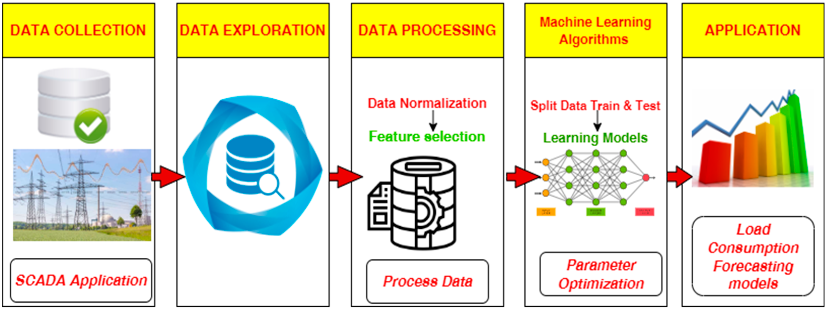
3.3. Forecasting Methodology

This section presents the proposed method to forecast short-term loads based on deep learning algorithms in a real dataset as illustrated in Figure 9. It begins with composing the dataset and describing preprocessing steps such as normalization and feature selection. Then building and training models: deep learning models to forecast short-term load based on historical data, namely: (LSTM, RNN, and GRU). After that, the hyperparameters tuning for machine learning models such as (optimizer, activation function, learning rate, number of epochs, batch size, and number of hidden layers) were used as well as the performance metrics to measure the accuracy of each model. Finally, select the best forecasting model. All models in this research were implemented using Python 3 with the Pandas, Seaborn, Sklearn, and Matplotlib, TensorFlow, and NumPy libraries. A 2.6 GHz intel core i5 processor platform with 8 GB of RAM running on a windows 10 desktop was used to implement this approach.

3.3.1. Data Preprocessing

Data preprocessing is a key stage in training the machine-learning model to use the ideal data structure; without preprocessed data, the machine-learning models may not operate as effectively as necessary, resulting in a miss and poor outcomes.

Depending on the nature of the raw data, different preprocessing sub-steps may be used [31], data normalization, and removing highly correlated features were used in this paper, as well as removing features with little correlation with the targeted feature, outlier’s removal, and an evaluation to check the null values in the original data. The techniques will be described in full in the next section.

Data Normalization

Data normalization is a preprocessing technique used to prevent some features from dominating all other features; data normalization aims for features with the same scale to be of equal importance; there are many types of data normalization methods, including standardization and max-min normalization [51]. The range of all features was standardized to be between [0–1] in this study, and the max-min normalization technique was used to conduct a linear transformation on the data, with the max-min normalization method determined using Equation (2) [52].

$$x^{\prime }=\frac{x-x_{min}}{x_{max}-x_{min}}$$

(2)

where x’ is the normalized value, x is the original feature value, x_min is the minimum value of the feature, and x_max is the maximum value of the feature.

Feature Selection

Feature selection is a technique where we choose those features in our data that contribute most to the target variable; it also has a good set of characteristics to achieve excellent identification rates in challenging situations [53]. The correlation between features was calculated, where its statistical technique determines how one variable moves/changes about the other variable, when we have highly correlated features in the dataset it increases the variance and is unreliable [54]. To isolate the highly correlated feature and the features with little correlation with the target; we used the filter method feature selection which depends on the correlation coefficient to apply a threshold to remove the features with a correlation higher than 90%.

3.3.2. Machine Learning Algorithms

In this section, we will provide a quick overview of the chosen three ML algorithms. The algorithms were chosen based on their popularity and performance in prior studies. Although sharing the same goals, an extensive range of ML deep learning algorithms has quite distinct mathematical models, strengths, and drawbacks. The deep learning method explores the relationships between the elements throughout the deep learning process so that the dependent variable value may be predicted by the independent variable. In this research LSTM, RNN, and GRU were used to forecast power consumption.

Long Short-Term Memory Model

A long short-term memory network (LSTM) is a sort of temporal cyclic neural network [55] that is specifically designed to address the long-term reliance issue that exists in a general RNN (recurrent neural network). Memory units replace the hidden layer neurons of a standard RNN network in an LSTM network. The memory unit’s architecture, which contains the input gate, forgetting gate, and output gate, can cause the networks to erase erroneous data or keep critical data at each time step.

Because of its capacity to learn temporal correlations, an LSTM recurrent network has become one of the best candidate networks in various domains such as language translation and speech recognition. Such timing correlates are common in power consumption loads because they are based on inhabitants’ behavior, which is difficult to understand and forecast. In the instance of electrical load forecasting, the LSTM network is intended to extract the phases of the loads from the patterns of the incoming power consumption profile, then store these states in memory, and lastly forecast based on the learned knowledge [48]. Figure 10 shows the construction of an LSTM cellblock.

Figure 10 shows the input gate acts like a filter, blocking out any input that is not relevant to the unit. The forget gate helps the unit forget any information previously stored in its memory. This helps the unit to focus on the new information it is receiving. The output gate is responsible for deciding whether or not the contents of the memory cell at the LSTM unit’s output should be revealed. It can either expose the contents or not reveal them. This gate has a sigmoid activation function, which means it can only output a value between 0 and 1. This helps to limit the output of the gate.

Recurrent Neural Network Model

Recurrent neural networks (RNNs) were designed to analyze time-series data and have been applied successfully in a variety of disciplines, including voice recognition, machine translation, and picture captioning [56,57]. RNN processes incoming sequence/time-series data by individual vectors at each step, keeping the information recorded at previous time steps concealed.

Figure 11 shows, “x” represents the input layer, “h” represents the hidden layer, and “y” represents the output layer. The networking variables A, B, and C were employed to enhance the model’s outputs. The current input is a mixture of input at x(t) and x(t) at every particular time t. (t − 1). At each particular time, the output was retrieved back to the network to enhance it.

Gate Recurrent Unit Model

The gated recurrent units (GRUs) are a gating method in recurrent neural networks established in 2014 [58]. The GRU is similar to a long short-term memory (LSTM) with a forget gate but has fewer parameters since it lacks an output gate. Ref. [59] GRU outperformed LSTM on specific tasks such as polyphonic music modeling, speech signal modeling, and natural language processing [60,61]. GRUs have been demonstrated to perform better on smaller and less frequent datasets [62]. GRU, which is an improvement on the classic RNN’s hidden layer, is depicted schematically and structurally in Figure 12. A GRU is made up of three gates: an update gate, a reset gate, and a temporary output. The associated symbols are as follows:

• Variable x_t is the network input at moment t.
• Variables h_t and ($\overline{ht}$) are information vectors that reflect the temporary output and the hidden layer output at instant t, respectively.
• Variables z_t and r_t are gate vectors that reflect the output of the update gate and the reset gate at moment t, respectively.
• The sigmoid and tanh activation functions are represented by (X) and tanh (x), respectively.

3.3.3. Hyperparameters Tuning for Machine Learning Models

This section will show the hyperparameters that were used in this research to obtain the best results for the models that have been applied. Discovering this section, we will investigate what the best parameters that determine the structure of models to predict electrical loads are, which is called hyperparameter tuning.

Tuning is the process of choosing an optimal set of hyperparameters for the learning algorithm [63]. The parameters used in this research are listed as follows:

• Best optimizer.
• Activation function.
• Learning rate.
• The number of epochs.
• Batch size.
• The number of hidden layers.
• Dropout.

3.3.4. Metrics Selection

Several metrics associated with data regression statistically measure its performance [64]. This paper will focus on the following metrics for deep learning models, namely: Mean Square Error (MSE), Root Mean Square Error (RMSE), Mean Absolute Error (MAE), and the coefficient of Determination (R-squared). This is to test these models and choose the best one based on the performance metrics listed below:

• Mean Square Error (MSE) is a calculation of the mean squared deviation between observed and predicted values. Equation (3) shows how to calculate MSE.

  $$\mathrm{MSE}=\frac{1}{n}{\displaystyle \sum }_{i=1}^n(\left|yt-y{t}^P\right|$$

  (3)

  where $yt$ is the actual data value and $y{t}^P$ the predicted data value.
• Root Mean Square Error (RMSE) is equal to the square root of the average squared error. Equation (4) shows how to calculate RMSE.

  $$\mathrm{RMSE}=\sqrt{\frac{1}{n}{\displaystyle \sum }_{i=1}^n{(\left|yt-y{t}^P\right|)}^2}$$

  (4)
• Mean Absolute Error (MAE) is the mean of the absolute value of the errors. Equation (5) shows how to calculate MAE.

  $$MAE=\frac{1}{n}{\displaystyle \sum }_{i=1}^n\left(\left|y_{i-}{y}_i^{^}\right|\right)$$

  (5)
• The coefficient of Determination (R-squared) is a number between 0 and 1 that measures the accuracy with which a model can anticipate a given result. Equation (6) shows how to calculate R-squared.

  $$coefficient of determination\left(R^2\right)=1-\frac{S{S}_{regression}}{S{S}_{total}}$$

  (6)

  where:

• $S{S}_{regression}$—The regression sum of squares (explained sum of squares).
• $S{S}_{total}$—The sum of all squares.

4. Result and Discussion

After deploying the models (LSTM, RNN, and GRU), the performance metrics are used to evaluate the models’ efficiency. In this section, we will illustrate the forecasting results of the machine learning algorithms as well as the performance metrics that rely on calculating the MSE, R-squared, RMSE, and MAE, for each algorithm.

4.1. Forecasting Results

This section will explain the method used to obtain the best results in the forecasting process in each model and it can be explained based on the following: (1) the best number of hidden layers, (2) batch size, (3) learning rate, (4) type of optimizer, and (5) type of activation function. In the beginning, the three models (LSTM, RNN, and GRU) were applied to a training rate of 70% and a test of 30%, to more than one type of optimizer on each model with a different learning rate to obtain the best results. The following sections will discuss the results obtained from different types of optimizers having different numbers of hidden layers.

4.1.1. Forecasting Using LSTM, RNN, and GRU Algorithms with Adam Optimizer

In this section, the results obtained from LSTM, RNN, and GRU algorithms will be discussed using one and multiple hidden layers in addition to the input and output layer on each model with the dropout in Adam optimizer.

Figure 13 shows the actual (blue) and the predicted (orange) results in forecasting the STLF using the LSTM, GRU, and RNN models. Where the test result values were taken from each learning rate. After comparing the test results for each learning rate in the LSTM model, it was found that the LSTM model achieved the highest value at a learning rate of 0.1, where R-squared = 0.87239, It can be seen from the error rate in forecasting the loads on the peak is minimal. The GRU model achieved the highest value at the learning rate of 0.01, where R-squared = 0.8732, the error rate in forecasting the loads on the peak is minimal, and the results are very close to the LSTM model. After comparing the test results for each learning rate in the RNN model, it was found that the RNN model achieved the highest value at a learning rate of 0.01, where R-squared = 0.86647.

Figure 14 shows the actual and predicted results of forecasting the STLF using the LSTM, GRU, and RNN models. Where the test result values were taken from each learning rate. After comparing the test results for each learning rate in the LSTM model, it was found that the LSTM model achieved the highest value at a learning rate of 0.01, where R-squared = 0.8672. The GRU model achieved the highest value at a learning rate of 0.01, where R-squared = 0.90228. The RNN model achieved the highest value at a learning rate of 0.001, where R-squared = 0.8275. It is concluded that the GRU model achieved the highest accuracy and the lowest error rate.

Table 3. Result from Adam optimizer for each model.

Learning Rate	Model	MSE	R-Squared	RMSE	MAE
One hidden layer
0.01	LSTM	0.00282	0.87239	0.05310	0.03937
0.001		0.00400	0.81900	0.06324	0.04786
0.01	GRU	0.00374	0.83063	0.06118	0.04731
0.001		0.00280	0.87323	0.05293	0.03790
0.01	RNN	0.00295	0.86647	0.05432	0.04115
0.001		0.00307	0.86104	0.05541	0.04065
Two hidden layers
0.01	LSTM	0.00293	0.8672	0.05417	0.04001
0.001		0.002988	0.864808	0.054662	0.04107
0.01	GRU	0.00215	0.90228	0.04647	0.03266
0.001		0.0028	0.8727	0.0530	0.0384
0.01	RNN	0.01529	0.30793	0.12367	0.10960
0.001		0.0038	0.8275	0.0617	0.0490
Three hidden layers
0.01	LSTM	0.00378	0.82861	0.06154	0.04779
0.001		0.00312	0.85855	0.05591	0.04233
0.01	GRU	0.00265	0.88001	0.05149	0.03738
0.001		0.00275	0.87547	0.05246	0.03790
0.01	RNN	0.01614	0.26963	0.12705	0.10554
0.001		0.00432	0.80448	0.06573	0.05348

shows the test results after applying each model based on the hyperparameter (Learning rate, number of hidden layers). The LSTM model achieved the best result when applied one hidden layer and a learning rate of 0.01, where the R- square is 0.87239. The best result of R-squared is 0.87239 in the GRU model at two hidden layers and the learning rate is 0.01. The RNN model obtains the best R-squared = 0.86647 at one hidden layer and the learning rate is 0.01. All in all, the best model that achieved the lowest error rate is GRU with a rate of learning equal to 0.01 and two hidden layers.

After applying the Adam optimizer in more than one way (one hidden layer, two hidden layers, and three hidden layers) with machine learning models LSTM, RNN, and GRU. Conclude this optimizer was applied with two hidden layers With the GRU model, gave the best results, as the R-squared was 90.228%, RMSE is 0.04647, and the MAE was 0.03266.

4.1.2. Forecasting Using LSTM, RNN, and GRU Algorithms with AdaGrad Optimizer

In this section, the results obtained from LSTM, RNN, and GRU algorithms will be discussed using one and multiple hidden layers in addition to the input and output layer on each model with the dropout in AdaGrad optimizer.

Figure 15 shows the actual and predicted results in forecasting the STLF using the LSTM, GRU, and RNN models. Where the test result values were taken from each learning rate. After comparing the test results for each learning rate in the LSTM model, it was found that the LSTM model achieved the highest value at a learning rate of 0.1, where R- square = 0.86627. It can be seen from Figure 15 that the error rate in forecasting the loads on the peak is minimal. The GRU model achieved the highest value at the learning rate of 0.01, where R- square = 0.86413, the results are very close to the LSTM model. The RNN model achieved the highest value at the learning rate of 0.01, where R- square = 0.86399, the results are very close to the LSTM and GRU models.

Figure 16 shows the actual and predicted results in forecasting the STLF using the LSTM, GRU, and RNN models. Where the test result values were taken from each learning rate. After comparing the test results for each learning rate in the LSTM model, it was found that the LSTM model achieved the highest value at a learning rate of 0.1, where R-squared = 0.8600. It can be seen from Figure 16, the error rate in forecasting the loads on the peak is very small, but there is a clear difference between the actual and forecasted values at the bottom (the electricity demand is minimal) in this model. The GRU model achieved the highest value at the learning rate of 0.01, where R-squared = 0.8672. The RNN model achieved the highest value at the learning rate of 0.01, where R-square = 0.8587. It can be seen from Figure 16, that there is a clear difference between the actual and forecasted values at the bottom (the electricity demand is minimal) in the RNN model, and the same case in their peak values.

Table 4. Result from AdaGrad optimizer for each model.

Learning Rate	Model	MSE	R-Squared	RMSE	MAE
One hidden layer
0.01	LSTM	0.00295	0.86627	0.05436	0.04305
0.001		0.00822	0.62783	0.09069	0.07237
0.01	GRU	0.00319	0.85533	0.05654	0.04119
0.001		0.00300	0.86413	0.05479	0.04042
0.01	RNN	0.00303	0.86273	0.05508	0.04251
0.001		0.00320	0.86399	0.05489	0.04171
Two hidden layers
0.01	LSTM	0.0030	0.8600	0.0556	0.0436
0.001		0.0215	0.0263	0.1466	0.1171
0.01	GRU	0.0035	0.8378	0.0598	0.0444
0.001		0.0029	0.8672	0.0541	0.0399
0.01	RNN	0.0040	0.8148	0.0639	0.0522
0.001		0.0031	0.8587	0.0558	0.0429
Three hidden layers
0.01	LSTM	0.02191	0.00837	0.14804	0.11889
0.001		0.02224	−0.0066	0.14916	0.11908
0.01	GRU	0.00405	0.81659	0.06366	0.04953
0.001		0.00301	0.86373	0.05487	0.04083
0.01	RNN	0.00908	0.58907	0.09530	0.08068
0.001		0.00329	0.85094	0.05739	0.04482

shows the test results after applying each model based on the hyperparameter (Learning rate, number of hidden layers). The LSTM model achieved the best result when applied one hidden layer and a learning rate of 0.01, where the R-squared is 0.87239. The best result of R-squared is 0.87239 in the GRU model at two hidden layers and the learning rate is 0.01. The RNN model obtains the best R-squared = 0.86647 at one hidden layer and the learning rate is 0.01. All in all, the best model that achieved the lowest error rate is GRU with a rate of learning equal to 0.01 and two hidden layers.

After applying the Adam optimizer in more than one way (one hidden layer, two hidden layers, and three hidden layers) with machine learning models LSTM, RNN, and GRU. Conclude this optimizer was applied with two hidden layers With the GRU model, gave the best results, as the R-squared was 90.228%, RMSE is 0.04647, and the MAE was 0.03266.

4.1.3. Forecasting Using LSTM, RNN, and GRU Algorithms with RMSprop Optimizer

In this section, the results obtained from LSTM, RNN, and GRU algorithms will be discussed using one and multiple hidden layers in addition to the input and output layer on each model with the dropout in RMSprop optimizer.

Figure 17 shows the actual and predicted results in forecasting the STLF using the LSTM, GRU, and RNN models. Where the test result values were taken from each learning rate. After comparing the test results for each learning rate in the LSTM model, it was found that the LSTM model achieved the highest value at a learning rate of 0.01, where R-squared = 0.84209. It can be seen from Figure 17, there is an error rate in the difference between the real and forecasted loads, where the accuracy rate in the small loads (minimum load) is not high. The GRU model achieved the highest value at a learning rate of 0.01, where R-squared = 0.87749, the error rate in forecasting the loads on the peak is very low, but there is a very small difference in the minimum loads. The RNN model achieved the highest value at a learning rate of 0.01, where R-squared = 0.85114, the results are very close to the GRU model.

Figure 18 shows the actual and predicted results in forecasting the STLF using the LSTM, GRU, and RNN models. Where the test result values were taken from each learning rate. After comparing the test results for each learning rate in the LSTM model, it was found that the LSTM model achieved the highest value at a learning rate of 0.001, where R-squared = 0.8216. It can be seen from Figure 18, the error rate in forecasting the loads on the peak is high, but there is a clear difference between the actual and forecasted values at the bottom and the peak loads (the electricity demand is minimal) in the LSTM model. Where the LSTM model was able to forecast the average loads in this case, as for the electrical loads at the top and the small loads, the model was not able to forecast their loads, and this led to a high error rate and a lack of accuracy for this model in this case. The GRU model achieved the highest value at a learning rate of 0.01, where R-squared = 0.8804, and the error rate in forecasting the loads on the peak and minimum loads is very low. The RNN model achieved the highest value at the learning rate of 0.01, where R-squared = 0.7915, which is a clear difference between the actual and forecasted values at the bottom (the electricity demand is minimal) are small in the RNN model, and the same case in the last test period, there is a fluctuation in the difference between the two values.

Table 5. Result from RMSprop optimizer for each model.

Learning Rate	Model	MSE	R-Squared	RMSE	MAE
One hidden layer
0.01	LSTM	0.00349	0.84209	0.05907	0.04313
0.001		0.00350	0.84130	0.05922	0.04489
0.01	GRU	0.00270	0.87749	0.05203	0.03904
0.001		0.00354	0.83976	0.05951	0.04310
0.01	RNN	0.00329	0.85114	0.05735	0.04446
0.001		0.00335	0.84833	0.05789	0.04609
Two hidden layers
0.01	LSTM	0.0080	0.6367	0.0895	0.0749
0.001		0.0039	0.8216	0.0627	0.0493
0.01	GRU	0.0026	0.8804	0.0513	0.0378
0.001		0.0032	0.8520	0.0571	0.0410
0.01	RNN	0.0046	0.7915	0.0678	0.0562
0.001		0.0046	0.7889	0.0683	0.0556
Three hidden layers
0.01	LSTM	0.00422	0.80874	0.06501	0.04828
0.001		0.00683	0.69075	0.08267	0.06936
0.01	GRU	0.00288	0.86941	0.05372	0.04146
0.001		0.00334	0.84857	0.05785	0.04172
0.01	RNN	0.01341	0.39317	0.11581	0.09153
0.001		0.00961	0.56479	0.09807	0.08433

shows the test results after applying each model based on the hyperparameter (Learning rate, number of hidden layers). The LSTM model achieved the best result when applied one hidden layer and a learning rate of 0.01, where the R-squared is 0.84209. The best result of R-squared is 0.8804 in the GRU model at two hidden layers and the learning rate is 0.01. The RNN model obtains the best R-squared = 0.85114 at one hidden layer and the learning rate is 0.01. All in all, the best model that achieved the lowest error rate is GRU with a rate of learning equal to 0.01 and two hidden layers, and the results of the LSTM and RNN algorithms were convergent when applying a single hidden layer.

After applying the RMSprop optimizer in more than one way (one hidden layer, two hidden layers, three hidden layers, different learning rates) with machine learning models LSTM, RNN, and GRU. Conclude this optimizer is applied with two hidden layers With the GRU model and the learning rate is 0.01, it gave the best results, as the R-squared was 88.02%, RMSE is 0.0513, and the MAE was 0.0378.

4.1.4. Forecasting Using LSTM, RNN, and GRU Algorithms with Adadelta Optimizer

In this section, the results obtained from LSTM, RNN, and GRU algorithms will be discussed using one and multiple hidden layers in addition to the input and output layer on each model with the dropout in Adadelta optimizer.

Figure 19 shows the actual and predicted results in forecasting the STLF using the LSTM, GRU, and RNN models. Where the test result values were taken from each learning rate. After comparing the test results for each learning rate in the LSTM model, it was found that the LSTM model achieved the highest value at a learning rate of 0.1, where R-squared = 0.81143. It can be seen from Figure 19, the difference between the actual and expected values can be seen, especially in the peak values in which the loads are the highest, and there is a large and clear difference between the expected and actual values, which led to an increase in the error rate in this case when the loads are minimal. The GRU model achieved the highest value at a learning rate of 0.1, where R-squared = 0.86781, and the error rate in forecasting the loads on the peak is very small, the RNN model obtained the best results compared to other models. The RNN model achieved the highest value at a learning rate of 0.1, where R-squared = 0.86348, and its results, in this case, are close to the results of the GRU model.

Figure 20 shows the actual and predicted results in forecasting the STLF using the LSTM, GRU, and RNN models. Where the test result values were taken from each learning rate. After comparing the test results for each learning rate in the LSTM model, it was found that the LSTM model achieved the highest value at a learning rate of 0.1, where R-squared = 0.7262. It can be seen from Figure 20, the error rate in forecasting the loads on the peak is high, but there is a clear difference between the actual and forecasted values at the bottom and the peak loads (the electricity demand is minimal) in the LSTM model. Where the LSTM model was able to forecast the average loads in this case, as for the electrical loads at the top and the small loads, the model was not able to forecast their loads, and this led to a high error rate and a lack of accuracy for this model in this case. The LSTM model in this case is considered a failure, and it cannot be relied upon in forecasting electrical loads because it has a large error rate and a low accuracy with a good estimate. The GRU model achieved the highest value at a learning rate of 0.1, where R-squared = 0.8676, and the error rate in forecasting the loads on the peak and minimum loads is very small. The RNN model achieved the highest value at a learning rate of 0.1, where R-squared = 0.8426, which is a slight difference between the actual and expected values in peak loads, especially at the end of the testing period, the difference was clear.

Table 6. Result from AdaDelta optimizer for each model.

Learning Rate	Model	MSE	R-Squared	RMSE	MAE
One hidden layer
0.01	LSTM	0.00416	0.81143	0.06455	0.05274
0.001		0.01577	0.28612	0.12561	0.10147
0.01	GRU	0.00292	0.86781	0.05405	0.04006
0.001		0.00959	0.56599	0.09794	0.07986
0.01	RNN	0.00301	0.86348	0.05492	0.04120
0.001		0.00586	0.73461	0.07658	0.06180
Two hidden layers
0.01	LSTM	0.0060	0.7262	0.0777	0.0603
0.001		0.0188	0.1487	0.1371	0.1092
0.01	GRU	0.0029	0.8676	0.0540	0.0397
0.001		0.0129	0.4138	0.1138	0.0923
0.01	RNN	0.0034	0.8426	0.0589	0.0441
0.001		0.0132	0.3993	0.1152	0.0912
Three hidden layers
0.01	LSTM	0.02018	0.03696	0.14205	0.11361
0.001		0.02253	−0.0198	0.15013	0.11925
0.01	GRU	0.00292	0.86749	0.05411	0.04024
0.001		0.01215	0.45025	0.11022	0.09018
0.01	RNN	0.00339	0.86348	0.05492	0.04120
0.001		0.01373	0.37867	0.11718	0.09260

shows the test results after applying each model based on the hyperparameter (learning rate, number of hidden layers). The LSTM model achieved the best result when applied one hidden layer and a learning rate of 0.01, where the R-squared is 0.81143. The best result of R-squared is 0.86781 in the GRU model at one hidden layer and the learning rate is 0.01. The RNN model obtains the best R-squared = 0.86348 at one hidden layer and the learning rate is 0.01. All in all, the best model that achieved the lowest error rate is GRU with a rate of learning equal to 0.01 and one hidden layer, and the results of the LSTM and RNN algorithms were convergent when applying a single hidden layer and the learning rate is 0.01.

After applying the AdaDelta optimizer in more than one way (one hidden layer, two hidden layers, three hidden layers, different learning rates) with machine learning models LSTM, RNN, and GRU. Conclude this optimizer is applied with one hidden layer With the GRU model and the learning rate is 0.1. In other words, the results were close between the different classes with a learning rate of 0.1, it gave the best results, as the R-squared was 86.781%, RMSE is 0.05405, and the MAE was 0.04006.

Figure 21 shows the results obtained by machine learning models from LSTM, RNN, and GRU on two hidden layers with a learning rate = 0.01. Here we only take the best results for comparison, and those applied to four optimizers (Adam, Adagrad, RMSprop, and AdaDelta). In general, the best optimizer gave the lowest percentage of MAE (Adam enhancer using GRU). However, the AdaDelta enhancer was the worst in terms of the high error rate compared to the other. Figure 21 also shows that in Adam’s optimizer using GRU model was the best where MAE = 0.03266.

In this section, all the results obtained from the proposed deep-learning methods for forecasting short-term electrical loads are discussed and explained. Performance metrics were based on R-squared, MAE, RMSE, and MSE to compare machine-learning algorithms (LSTM, RNN, and GRU) and choose the best among them. In addition, we have applied more than one hidden layer, more than one learning rate, and four optimizations to choose the best and obtain the lowest error rate. The GRU model obtained the best results, where the R-squared value = 90.2% and MAE = 0.03266, RMSE = 0.04647. That is when applying Adam’s enhancer and two hidden layers with a learning ratio of 0.01. Where many batch sizes and the number of epochs were tested, and the best batch size was 32 and the number of epochs was 50, with a training rate is 70% and a test is 30%. In

Table 7. Results from previous studies.

Reference	Algorithms	Result	Location
[29]	NN with PSO algorithm	MAPE = 0.0338, MAE = 0.02191.	Iran.
[30]	EMD-GRU-FS	Accuracy on four data sets was 96.9%, 95.31%, 95.72%, and 97.17%, consecutively.	Public
[31]	LSTM with EMD	MAPE = 2.6249% in the winter and 2.3047% in the summer.	Public
[32]	VMD, LSTM with optimizer BOA, SVR, LR, RF, and EMD-LSTM	The LSTM with optimizer BOA gave the best, where MAPE is 0.4186%.	China
[33]	VMD, TCN	MAPE for 6-, 12-, and 24-step forecasting is 0.274%, 0.326%, and 0.405, respectively	Global Energy Competition 2014
[35]	ANN based on the Levenberg Marquardt and newton algorithms	The model is a perfect fitting with a rate of 90% of the variance in the power consumption variable predicted from the independent variable.	Public
[36]	NARX and ANN	MAPE and RMSE of 3.16% and 270.60, respectively.	Algerian
[37]	NARX, SVR	The SVR outperformed the NARX neural network model, for the day ahead, a week ahead, and a month ahead forecasting, the average predicting accuracy is approximately 91%, 88–90%, and 85–87%, respectively.	Public
[38]	MFRFNN	The RMSE for wind speed prediction, Google stock price prediction, and air quality index prediction are decreased by 35.12%, 13.95%, and 49.62, respectively.	Real Datasets
[39]	EANN, BANN	EANN is the best, where RMSE = 296.3437, MAPE = 15.9396. In BANN given the result, RMSE = 309.6022, and MAPE = 16.236.	France
[40]	RNN	MAE = 0.24, 0.12 straight for 50 h ago and an hour ago.	London
[41]	LSTM, ISCOA	STLF give MAE = 0.0733, MAPE = 5.1882, MSE = 0.0115, RMSE = 0.1076.	India-Mumbai
[42]	DLSF, SVM	The DLSF model outperformed the SVM algorithm, where the accuracy of DLSF is 90%, and SVM = 70%.	China
[43]	PDRNN, ARIMA, SVR, and RNN.	The PDRNN method outperforms ARIMA, SVR, and RNN, where RMSE (kWh) = 0.4505, 0.5593, 0.518, and 0.528 respectively.	Ireland
[45]	CNN, SVM, ANN, and LSTM.	The superiority of the proposed model CNN over SVM, ANN, and LSTM where RMSE = 0.677, 0.814, 0.691, 0.7 respectively.	Public
[46]	NN with Bayesian networks	MAE is 1.0085, and MAAPE is 0.5035.	Irish
[48]	LSTM, BPNN, KNN,	The LSTM with ELM is the best where MAPE = 8.18%.	China

we will discuss and present the results obtained from previous studies and compare them with the results obtained in our study as illustrated below:

From Table 7 it can be seen that the outcomes from each study are different in which this is based on many factors namely; dataset, features, algothims used and tunning parameters. As an overall, our study shows better results when the GRU model is applied with MSE of 0.00215, RMSE of 0.04647, and MAE of 0.03266. This is due to the use of seven Hyperparameters in tuning the models in order to obtain the best results and avoid overfitting.

5. Conclusions and Future Work

In this research, three deep learning algorithms (LSTM, GRU, and RNN) were used to forecast the electrical loads based on the readings that were taken from the SCADA program in the Electricity Company of the Tubas area in Palestine. Forecasting is an essential requirement for any country in the world to improve future planning. It is the science of the economical amount of electric power for a utility company. It must be as accurate as possible, reliable, and meaningful. The proposed models are aiming to bridge the gap between the demand and the energy, reduce electricity losses from large quantities, and plan the future of infrastructure more accurately.

The GRU model achieved the best performance as it achieved the highest accuracy and the lowest error rate. In addition, many improvements were used in building models such as the use of different types of optimizers. Simulation results found that Adam achieved the best performance for the GRU model. As the model and data were applied to a hidden layer and multiple hidden layers, the use of two hidden layers in predicting electrical loads achieved the best performance. The best GRU model achieved results of R-squared 90.228%, MSE of 0.00215, MAE of 0.03266, and RMSE of 0.04647.

Exploratory data analysis reveals that temperature plays a large and influential factor in loads. Moreover, this research has proven that in the late night hours and early morning hours, consumption and loads are minimal, because all factories, institutions, and homes are closed. It was noted that in the winter, the loads are low, because the irrigation of crops relies on rainwater, and there is no need to operate wells that depend on electricity. This research also has many practical implications. First, it provides methodology of creating deep learning models that can be used by electric companies and allowing costs to be reduced. Second, it provides a more accurate STLF, and this will reduce planning uncertainty.

As a plan for future work, we recommend creating a model capable of predicting electrical loads based on the available and recommended new features such as humidity, reading all consumption from homes through smart meters, and training the model online based on the data obtained from these smart meters. This will help in revealing the behavior of the electric load consumption in the country. In addition, we are planning to build web interfaces that display all the expected loads for the concerned department, as well as forecasting the long-term electrical loads.

References

1. Yohanandhan, R.V.; Elavarasan, R.M.; Pugazhendhi, R.; Premkumar, M.; Mihet-Popa, L.; Zhao, J.; Terzija, V. A specialized review on outlook of future Cyber-Physical Power System (CPPS) testbeds for securing electric power grid. Int. J. Electr. Power Energy Syst. 2022, 136, 107720. [Google Scholar] [CrossRef]
2. Azarpour, A.; Mohammadzadeh, O.; Rezaei, N.; Zendehboudi, S. Current status and future prospects of renewable and sustainable energy in North America: Progress and challenges. Energy Convers. Manag. 2022, 269, 115945. [Google Scholar] [CrossRef]
3. Huang, N.; Wang, S.; Wang, R.; Cai, G.; Liu, Y.; Dai, Q. Gated spatial-temporal graph neural network based short-term load forecasting for wide-area multiple buses. Int. J. Electr. Power Energy Syst. 2023, 145, 108651. [Google Scholar] [CrossRef]
4. Liu, C.-L.; Tseng, C.-J.; Huang, T.-H.; Yang, J.-S.; Huang, K.-B. A multi-task learning model for building electrical load prediction. Energy Build. 2023, 278, 112601. [Google Scholar] [CrossRef]
5. Xia, Y.; Wang, J.; Wei, D.; Zhang, Z. Combined framework based on data preprocessing and multi-objective optimizer for electricity load forecasting. Eng. Appl. Artif. Intell. 2023, 119, 105776. [Google Scholar] [CrossRef]
6. Jena, T.R.; Barik, S.S.; Nayak, S.K. Electricity Consumption & Prediction using Machine Learning Models. Acta Tech. Corviniensis-Bull. Eng. 2020, 9, 2804–2818. [Google Scholar]
7. Mansouri, S.A.; Jordehi, A.R.; Marzband, M.; Tostado-Véliz, M.; Jurado, F.; Aguado, J.A. An IoT-enabled hierarchical decentralized framework for multi-energy microgrids market management in the presence of smart prosumers using a deep learning-based forecaster. Appl. Energy 2023, 333, 120560. [Google Scholar] [CrossRef]
8. Oprea, S.-V.; Bâra, A.; Puican, F.C.; Radu, I.C. Anomaly Detection with Machine Learning Algorithms and Big Data in Electricity Consumption. Sustainability 2021, 13, 10963. [Google Scholar] [CrossRef]
9. Lei, L.; Chen, W.; Wu, B.; Chen, C.; Liu, W. A building energy consumption prediction model based on rough set theory and deep learning algorithms. Energy Build. 2021, 240, 110886. [Google Scholar] [CrossRef]
10. Liu, T.; Xu, C.; Guo, Y.; Chen, H. A novel deep reinforcement learning based methodology for short-term HVAC system energy consumption prediction. Int. J. Refrig. 2019, 107, 39–51. [Google Scholar] [CrossRef]
11. Al-Bayaty, H.; Mohammed, T.; Wang, W.; Ghareeb, A. City scale energy demand forecasting using machine learning based models: A comparative study. ACM Int. Conf. Proceeding Ser. 2019, 28, 1–9. [Google Scholar]
12. Ahmad, T.; Chen, H.; Huang, R.; Yabin, G.; Wang, J.; Shair, J.; Akram, H.M.A.; Mohsan, S.A.H.; Kazim, M. Supervised based machine learning models for short, medium and long-term energy prediction in distinct building environment. Energy 2018, 158, 17–32. [Google Scholar] [CrossRef]
13. Geetha, R.; Ramyadevi, K.; Balasubramanian, M. Prediction of domestic power peak demand and consumption using supervised machine learning with smart meter dataset. Multimedia Tools Appl. 2021, 80, 19675–19693. [Google Scholar] [CrossRef]
14. Chen, C.; Liu, Y.; Kumar, M.; Qin, J.; Ren, Y. Energy consumption modelling using deep learning embedded semi-supervised learning. Comput. Ind. Eng. 2019, 135, 757–765. [Google Scholar] [CrossRef]
15. Khan, Z.; Adil, M.; Javaid, N.; Saqib, M.; Shafiq, M.; Choi, J.-G. Electricity Theft Detection Using Supervised Learning Techniques on Smart Meter Data. Sustainability 2020, 12, 8023. [Google Scholar] [CrossRef]
16. Kaur, H.; Kumari, V. Predictive modelling and analytics for diabetes using a machine learning approach. Appl. Comput. Inform. 2022, 18, 90–100. [Google Scholar] [CrossRef]
17. Kim, T.-Y.; Cho, S.-B. Predicting residential energy consumption using CNN-LSTM neural networks. Energy 2019, 182, 72–81. [Google Scholar] [CrossRef]
18. Wang, Z.; Srinivasan, R.S. A Review of Artificial Intelligence Based Building Energy Use Prediction: Contrasting the Capabilities of single and Ensemble Prediction Models. Renew. Sustain. Energy Rev. 2017, 75, 796–808. [Google Scholar] [CrossRef]
19. Ivanov, D.; Tsipoulanidis, A.; Schönberger, J. Global Supply Chain and Operations Management; Springer International Publishing: Cham, Switzerland, 2017. [Google Scholar]
20. Kuster, C.; Rezgui, Y.; Mourshed, M. Electrical load forecasting models: A critical systematic review. Sustain. Cities Soc. 2017, 35, 257–270. [Google Scholar] [CrossRef]
21. Arora, S.; Taylor, J.W. Rule-based autoregressive moving average models for forecasting load on special days: A case study for France. Eur. J. Oper. Res. 2018, 266, 259–268. [Google Scholar] [CrossRef] [Green Version]
22. Takeda, H.; Tamura, Y.; Sato, S. Using the ensemble Kalman filter for electricity load forecasting and analysis. Energy 2016, 104, 184–198. [Google Scholar] [CrossRef]
23. Maldonado, S.; González, A.; Crone, S. Automatic time series analysis for electric load forecasting via support vector regression. Appl. Soft Comput. 2019, 83, 105616. [Google Scholar] [CrossRef]
24. Rendon-Sanchez, J.F.; de Menezes, L.M. Structural combination of seasonal exponential smoothing forecasts applied to load forecasting. Eur. J. Oper. Res. 2019, 275, 916–924. [Google Scholar] [CrossRef]
25. Lindberg, K.; Seljom, P.; Madsen, H.; Fischer, D.; Korpås, M. Long-term electricity load forecasting: Current and future trends. Util. Policy 2019, 58, 102–119. [Google Scholar] [CrossRef]
26. Hong, T.; Forecasting, S.F. Probabilistic electric load forecasting: A tutorial review. Int. J. Forecast. 2016, 32, 914–938. [Google Scholar] [CrossRef]
27. Kloker, S.; Straub, T.; Weinhardt, C.; Maedche, A.; Brocke, J.V.; Hevner, A. Designing a Crowd Forecasting Tool to Combine Prediction Markets and Real-Time Delphi. In Lecture Notes in Computer Science; Springer: Cham, Switzerland, 2017; Volume 10243, pp. 468–473. [Google Scholar] [CrossRef]
28. Goehry, B.; Goude, Y.; Massart, P.; Poggi, J.-M. Aggregation of Multi-Scale Experts for Bottom-Up Load Forecasting. IEEE Trans. Smart Grid 2019, 11, 1895–1904. [Google Scholar] [CrossRef]
29. Chafi, Z.S.; Afrakhte, H. Short-Term Load Forecasting Using Neural Network and Particle Swarm Optimization (PSO) Algorithm. Math. Probl. Eng. 2021, 2021, 5598267. [Google Scholar] [CrossRef]
30. Gao, X.; Li, X.; Zhao, B.; Ji, W.; Jing, X.; He, Y. Short-Term Electricity Load Forecasting Model Based on EMD-GRU with Feature Selection. Energies 2020, 12, 1140. [Google Scholar] [CrossRef] [Green Version]
31. Yuan, B.; He, B.; Yan, J.; Jiang, J.; Wei, Z.; Shen, X. Short-term electricity consumption forecasting method based on empirical mode decomposition of long-short term memory network. IOP Conf. Ser. Earth Environ. Sci. 2022, 983, 12004. [Google Scholar] [CrossRef]
32. He, F.; Zhou, J.; Feng, Z.-K.; Liu, G.; Yang, Y. A hybrid short-term load forecasting model based on variational mode decomposition and long short-term memory networks considering relevant factors with Bayesian optimization algorithm. Appl. Energy 2019, 237, 103–116. [Google Scholar] [CrossRef]
33. Zhou, F.; Zhou, H.; Li, Z.; Zhao, K. Multi-Step Ahead Short-Term Electricity Load Forecasting Using VMD-TCN and Error Correction Strategy. Energies 2022, 15, 5375. [Google Scholar] [CrossRef]
34. Nasiri, H.; Ebadzadeh, M.M. Multi-step-ahead Stock Price Prediction Using Recurrent Fuzzy Neural Network and Variational Mode Decomposition. arXiv 2022, arXiv:2212.14687. [Google Scholar]
35. Biswas, M.R.; Robinson, M.D.; Fumo, N. Prediction of residential building energy consumption: A neural network approach. Energy 2016, 117, 84–92. [Google Scholar] [CrossRef]
36. Bendaoud, N.M.M.; Farah, N. Using deep learning for short-term load forecasting. Neural Comput. Appl. 2020, 32, 15029–15041. [Google Scholar] [CrossRef]
37. Thokala, N.K.; Bapna, A.; Chandra, M.G. A deployable electrical load forecasting solution for commercial buildings. In Proceedings of the 2018 IEEE International Conference on Industrial Technology (ICIT), Lyon, France, 20–22 February 2018; pp. 1101–1106. [Google Scholar]
38. Nasiri, H.; Ebadzadeh, M.M. MFRFNN: Multi-Functional Recurrent Fuzzy Neural Network for Chaotic Time Series Prediction. Neurocomputing 2022, 507, 292–310. [Google Scholar] [CrossRef]
39. Alobaidi, M.H.; Chebana, F.; Meguid, M.A. Robust ensemble learning framework for day-ahead forecasting of household based energy consumption. Appl. Energy 2018, 212, 997–1012. [Google Scholar] [CrossRef] [Green Version]
40. Fekri, M.N.; Patel, H.; Grolinger, K.; Sharma, V. Deep learning for load forecasting with smart meter data: Online Adaptive Recurrent Neural Network. Appl. Energy 2020, 282, 116177. [Google Scholar] [CrossRef]
41. Somu, N.; MR, G.R.; Ramamritham, K. A hybrid model for building energy consumption forecasting using long short term memory networks. Appl. Energy 2020, 261, 114131. [Google Scholar] [CrossRef]
42. Li, L.; Ota, K.; Dong, M. Everything is Image: CNN-based Short-Term Electrical Load Forecasting for Smart Grid. In Proceedings of the 2017 14th International Symposium on Pervasive Systems, Algorithms and Networks & 2017 11th International Conference on Frontier of Computer Science and Technology & 2017 Third International Symposium of Creative Computing (ISPAN-FCST-ISCC), Exeter, UK, 21–23 June 2017; Volume 99, pp. 344–351. [Google Scholar] [CrossRef]
43. Shi, H.; Xu, M.; Grid, R.L. Deep learning for household load forecasting—A novel pooling deep RNN. IEEE Trans. Smart Grid 2017, 8, 133–190. [Google Scholar]
44. Amarasinghe, K.; Marino, D.L.; Manic, M. Deep neural networks for energy load forecasting. In Proceedings of the 2017 IEEE 26th International Symposium on Industrial Electronics (ISIE), Edinburgh, UK, 19–21 June 2017; Volume 14, pp. 1483–1488. [Google Scholar]
45. Bache, K.; Lichman, M. UCI machine learning repository. IEEE Access 2018, 206, 23. [Google Scholar]
46. Bessani, M.; Massignan, J.A.; Santos, T.; London, J.B.; Maciel, C.D. Multiple households very short-term load forecasting using bayesian networks. Electr. Power Syst. Res. 2020, 189, 106733. [Google Scholar] [CrossRef]
47. Gong, L.; Yu, M.; Jiang, S.; Cutsuridis, V.; Pearson, S. Deep Learning Based Prediction on Greenhouse Crop Yield Combined TCN and RNN. Sensors 2021, 21, 4537. [Google Scholar] [CrossRef] [PubMed]
48. Kong, W.; Dong, Z.Y.; Jia, Y.; Hill, D.J.; Xu, Y.; Zhang, Y. Short-Term Residential Load Forecasting Based on LSTM Recurrent Neural Network. IEEE Trans. Smart Grid 2017, 10, 841–851. [Google Scholar] [CrossRef]
49. Javed, U.; Ijaz, K.; Jawad, M.; Ansari, E.A.; Shabbir, N.; Kütt, L.; Husev, O. Exploratory Data Analysis Based Short-Term Electrical Load Forecasting: A Comprehensive Analysis. Energies 2021, 14, 5510. [Google Scholar] [CrossRef]
50. Zhang, J.; Xu, Z.; Wei, Z. Absolute logarithmic calibration for correlation coefficient with multiplicative distortion. Commun. Stat. Comput. 2023, 52, 482–505. [Google Scholar] [CrossRef]
51. Aggarwal, C.C. Data Mining: The Textbook; Springer: Berlin/Heidelberg, Germany, 2015; Volume 1. [Google Scholar]
52. Punyani, P.; Gupta, R.; Kumar, A. A multimodal biometric system using match score and decision level fusion. Int. J. Inf. Technol. 2022, 14, 725–730. [Google Scholar] [CrossRef]
53. Vafaie, H.; De Jong, K. Genetic algorithms as a tool for feature selection in machine learning. ICTAI 2018, 200–203. [Google Scholar] [CrossRef]
54. Norouzi, A.; Aliramezani, M.; Koch, C.R. A correlation-based model order reduction approach for a diesel engine NOx and brake mean effective pressure dynamic model using machine learning. Int. J. Engine Res. 2020, 22, 2654–2672. [Google Scholar] [CrossRef]
55. Gers, F.A.; Schmidhuber, J.; Cummins, F. Learning to Forget: Continual Prediction with LSTM. Neural Comput. 2000, 12, 2451–2471. [Google Scholar] [CrossRef]
56. Goodfellow, I.; Bengio, Y.; Courville, A. Deep Learning; MIT Press: Cambridge, MA, USA, 2016. [Google Scholar]
57. Fan, C.; Wang, J.; Gang, W.; Li, S. Assessment of deep recurrent neural network-based strategies for short-term building energy predictions. Appl. Energy 2019, 236, 700–710. [Google Scholar] [CrossRef]
58. Cho, K.; Van Merrienboer, B.; Bahdanau, D.; Bengio, Y. On the properties of neural machine translation: Encoder-decoder approaches. arXiv 2019, arXiv:1409.1259. [Google Scholar] [CrossRef]
59. Britz, D. Recurrent neural network tutorial, part 4 implementing a gru/lstm rnn with python and Theano. Inf. Syst. E-bus. Manag. 2015, 256, 560–587. [Google Scholar]
60. Ravanelli, M.; Brakel, P.; Omologo, M.; Bengio, Y. Light Gated Recurrent Units for Speech Recognition. IEEE Trans. Emerg. Top. Comput. Intell. 2018, 2, 92–102. [Google Scholar] [CrossRef] [Green Version]
61. Su, Y.; Kuo, C.-C.J. On extended long short-term memory and dependent bidirectional recurrent neural network. Neurocomputing 2019, 356, 151–161. [Google Scholar] [CrossRef] [Green Version]
62. Gruber, N.; Jockisch, A. Are GRU Cells More Specific and LSTM Cells More Sensitive in Motive Classification of Text? Front. Artif. Intell. 2020, 3, 40. [Google Scholar] [CrossRef]
63. Veloso, B.; Gama, J.; Malheiro, B.; Vinagre, J. Hyperparameter self-tuning for data streams. Inf. Fusion 2021, 76, 75–86. [Google Scholar] [CrossRef]
64. Plevris, V.P.; Solorzano, G.S.; Bakas, N.B.; Seghier, M.E.A.B.S. Investigation of performance metrics in regression analysis and machine learning-based prediction models. IEEE Trans. Emerg. Top. Comput. Intell. 2022, 13, 1–40. [Google Scholar] [CrossRef]
Figure 1. Basic workflow for electric load forecasting models.
Energies 16 02283 g001
Figure 2. Correlation coefficient for all features in the dataset.
Energies 16 02283 g002
Figure 3. The demand for electric load in Kilowatts hours (kWh) from 2021 to 2022.
Energies 16 02283 g003
Figure 4. Distribution of electric load demand based on the days of the week.
Energies 16 02283 g004
Figure 5. Distribution of electric load demand based on the hours of the day.
Energies 16 02283 g005
Figure 6. Power demand (kWh) over time (Sep-2021 to Jun-2022).
Energies 16 02283 g006
Figure 7. Tubas electricity demand over time period (Sep-2021 to Jun-2022).
Energies 16 02283 g007
Figure 8. The relationship between temperature in degrees and the demand power in (kWh).
Energies 16 02283 g008
Figure 9. Methodology of building the machine learning algorithms for the electric load consumption.
Energies 16 02283 g009
Figure 10. A long short-term memory block diagram structure.
Energies 16 02283 g010
Figure 11. Recurrent Neural Network Structure.
Energies 16 02283 g011
Figure 12. Gate Recurrent Unit Structure.
Energies 16 02283 g012
Figure 13. Electricity load forecasting results for each model are based on the Adam optimizer and one hidden layer.
Energies 16 02283 g013
Figure 14. Electricity load forecasting results for each model are based on the Adam optimizer and two hidden layers.
Energies 16 02283 g014
Figure 15. Electricity load forecasting results for each model based on AdaGrad optimizer and one hidden layer.
Energies 16 02283 g015
Figure 16. Electricity load forecasting results for each model are based on the AdaGrad optimizer and two hidden layers.
Energies 16 02283 g016
Figure 17. Electricity load forecasting results for each model based on RMSprop optimizer and one hidden layer.
Energies 16 02283 g017
Figure 18. Electricity load forecasting results for each model are based on the RMSprop optimizer and two hidden layers.
Energies 16 02283 g018
Figure 19. Electricity load forecasting results for each model are based on Adadelta optimizer and one hidden layer.
Energies 16 02283 g019
Figure 20. Electricity load forecasting results for each model are based on AdaDelta optimizer and two hidden layers.
Energies 16 02283 g020
Figure 21. MAE results were obtained by LSTM, RNN, and GRU models with more than one optimizer.
Energies 16 02283 g021