Hypothesis

Stochastic Security-Constrained Economic Dispatch of Load-Following and Contingency Reserves Ancillary Service Using a Grid-Connected Microgrid during Uncertainty

by
Kalyani Makarand Kurundkar
* and
Geetanjali Abhijit Vaidya
Electrical Engineering Department, PVGs COET and GKPIM, Pune 411009, India
*
Author to whom correspondence should be addressed.
Energies 2023, 16(6), 2607; https://doi.org/10.3390/en16062607
Submission received: 27 December 2022 / Revised: 3 March 2023 / Accepted: 5 March 2023 / Published: 9 March 2023
(This article belongs to the Special Issue Optimization and Energy Management in Smart Grids)

Abstract

:
In the context of the growing penetration of renewable power sources in power systems causing probabilistic contingency conditions, a suitable economic dispatch model is decisively needed. There is a lack of research in the field of probabilistic mathematical formulation considering the uncertainties due to the stochastic nature of renewables and contingency occurrence, as it is a very complex problem to be solved. The most appropriate model is the stochastic security-constrained economic dispatch (SSCED) model for optimized economic dispatch decisions during uncertainty. However, because of its complexity, it is rarely employed. This paper attempts to solve the complex SSCED problem in the presence of the uncertainty of resources and probabilistic contingency conditions, which is a novel effort in this regard. The SSCED is carried out over multiple periods to provide the load-following or contingency reserves. In the proposed SSCED, the uncertainty problem is addressed by modeling the stochastic wind energy power source by using “probability transition scenarios”. The uncertainty caused by probabilistic contingency conditions in the dispatch schedule is approximated using a “state-specific transition matrix”. The frequency control reserves in contingency conditions are co-optimized with energy, and stochastic security-constrained economic dispatch is achieved. The efforts are put forward to suggest a new market model in the presence of the uncertainty of renewable energy availability. Case studies are examined to show the potential technical and financial advantages of the proposed SSCED through co-optimization. Grid-connected microgrid owners offer frequency control ancillary services by providing load-following ramping reserves in the normal state and contingency reserves in the state of contingency. The probabilistic contingencies considered are generator failure and an underloading condition. A modified “IEEE 30 bus system” is considered a grid-connected microgrid for testing the proposed SSCED. The results show that the greater the flexibility of the resources, the greater the technical and economic benefits. The increase in ramping flexibility of a wind source results in almost an 8.1% reduction in operational costs compared to the base case. The contingency condition analysis shows that the presence of ramping reserves in the system enhances the power system performance, avoiding the cascading effects that ultimately cause a power system failure.

1. Introduction

In order to maintain the voltage profile, stability, and security of the power system as well as to support the main grid, microgrids may offer possible ancillary services. Due to the increased prevalence of unreliable renewable energy sources, ancillary services have become crucial at the distribution level [1].
It is found from the literature that researchers have placed a greater emphasis on estimating spinning reserves from renewable sources and co-optimizing them with energy while taking into account frequency control ancillary services provided by microgrids [2,3,4,5]. The co-optimization of energy and reserves in presence of converter-controlled DERs by blockchain technology is discussed in [6]. The stochastic optimization of energy and reserves are considered in [7]; using scenarios, the model takes into account and incorporates uncertainties linked to the production of renewable energy, day-ahead market pricing, and costs associated with unbalanced energy. When comparing the outcomes of stochastic and deterministic models, the cost of stochastic planning is 5% less than that of deterministic planning. A deterministic co-optimization considers the bi-level coordinated dispatch model that fully takes into account the informational interactions between the main grid and active distribution network [8]. To reduce operating expenses, a day-ahead active power scheduling approach that takes into account the errors in forecasting for renewable energy is suggested [9]. Profit maximization through the co-optimization of energy and spinning reserves given by renewable sources and energy storage has been studied [10]. Security-Constrained Economic Dispatch (SCED) in the reserve allocation electricity market is discussed [11].
It has been observed that until now, the research work mainly focused on the co-optimization of energy and reserves considering the deterministic approach for economic dispatch. Much less research work has been carried out considering the stochastic co-optimization of energy and reserves under uncertainty.
Further, as inferred from the literature survey on the stochastic co-optimization of energy and reserves, it is found that although stochastic co-optimization is carried out by few researchers, addressing uncertainty due to renewables, the uncertainty due to probabilistic contingencies, is rarely considered. The research handling of both uncertainties, i.e., the uncertainty due to renewables and the uncertainty due to probabilistic contingency while performing stochastic co-optimization of energy and reserves, is hardly found as it is very complex. Worldwide, system operators are facing challenges in handling the complex problem of the uncertainty modeling of renewable resources and contingencies while co-optimizing the dispatch of energy with ramp reserves in normal and contingency conditions [12]. This issue can be solved by a systematic solution to the stochastic security-constrained economic dispatch which considers the uncertainty.
This research work contributes by addressing the issue of the stochastic security-constrained co-optimization of energy and reserves in the presence of uncertainty of resources along with probabilistic contingency occurrence, which is decisively needed.
This need is addressed in this research work, and it is novel since it focuses on:
  • Solving multiperiod SSCED by the co-optimization of energy and ramping reserves in both normal and contingency conditions.
  • Modeling the uncertainty of wind power output and solving the aforementioned complex problem using “probability-weighted scenarios and transition matrices” [13].
  • Modeling probabilistic contingency conditions.
  • Demonstrating the management of Fast Ramping (FR) resources, such as wind energy, and using its negative characteristic of power ramping into an advantageous one.
  • Validating the impact of change in the flexibility (ramping rate) of generators on active power costs in normal and contingency conditions.
The structure of this paper is as follows. The typical structure of the proposed SSCED multiperiod problem structure is described in Section 2, and Section 3 describes the proposed methodology for solving the multiperiod SSCED problem. The solution of case studies, outcomes, and results are discussed in Section 4. Section 5 concludes this investigation and suggests potential directions for future research work.

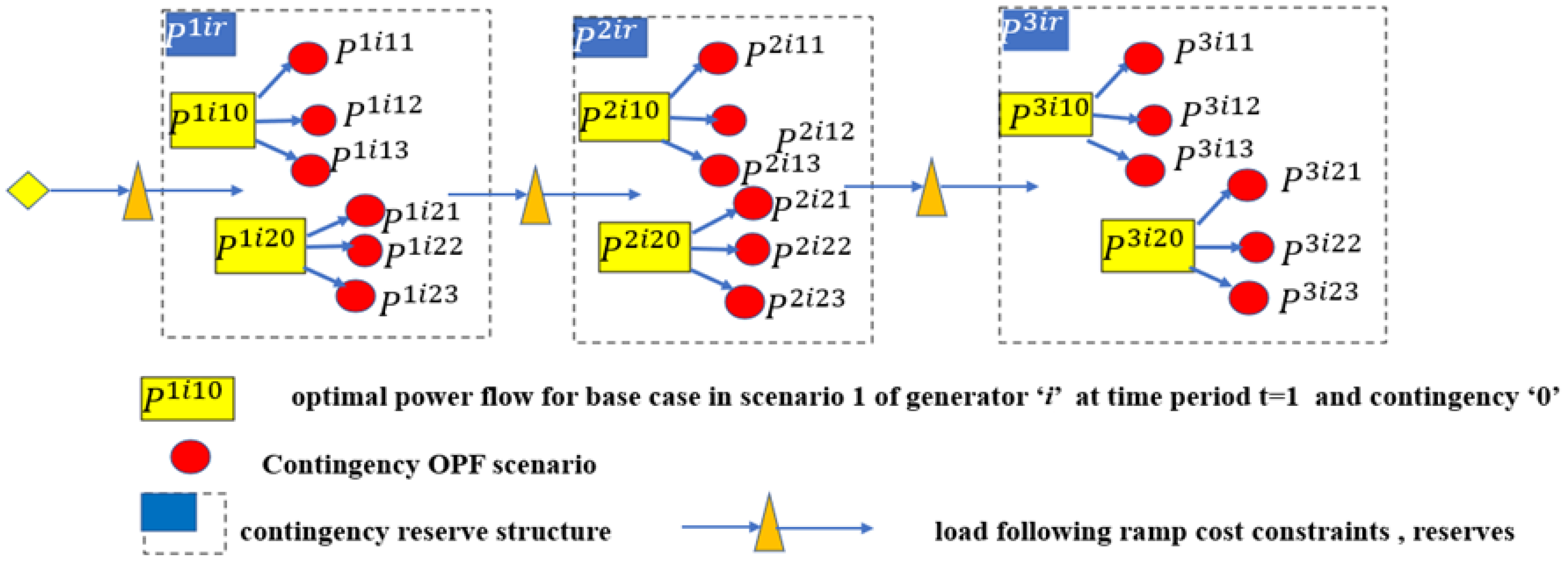
2. Typical Structure of Proposed SSCED Multiperiod Problem Structure

The basic active power dispatch in this work is represented as follows for the single and multiperiod problem structure of the SSCED. The active power dispatch P, from a resource i, renewable energy generation scenario s, and contingency state c, in time period t, has the indices as shown in Figure 1.

2.1. Single Base Scenario (Single Renewable Generation Profile)

The structure of the proposed single-period SSCED problem with a single base generation scenario under the proposed strategy is illustrated by the diagram in Figure 2. for the time period t = 1, the yellow-colored box is the power flow scenario for the base case P 1 i 10 , i.e., in the high-probability case in scenario s = 1, the dashed box shows the reference dispatch set P 1 i r . The red circles represent the power flow scenario for “low probability contingency states 1, 2…c” at time period t = 1, in generation scenario s = 1, for generator i, and are correspondingly P 1 i 11 , P 1 i 12 ……. P 1 i 1 c .
The ramp limits that prevent contingency state dispatches from deviating from the base case dispatch are shown by the blue colored arrows when contingencies 1, 2…, and c, occur.

2.2. Multiple Base Scenario (Multiple Renewable Generation Profile)

Similarly, for stochastic security-constrained economic dispatch, there are multiple renewable energy generation profiles considered. This creates multiple base case scenarios in a single time period t = 1, as shown in Figure 3. Two generation profiles are creating two generation scenarios and three probabilistic contingencies, i.e., c = 1, 2, and 3.
In the proposed stochastic multiperiod problem structure, there is a commitment schedule that is allotted to all states for simulating a variety of scenarios in the base case and contingency states for multiple periods, as shown in Figure 4.
It is more challenging to extend a problem over multiple periods. In order to ensure that the contingency state dispatches, the economic dispatch decisions are made before the occurrence of contingencies from the base case power flow scenario while adhering to ramp rate limits (blue colored arrows), as seen in Figure 4. Since the uncertainty is actually revealed period by period, this issue can be resolved by adopting a “Markovian structure” [14], where a stochastic model is characterized as a succession of potential events, where each event’s probability is solely dependent on the state that was attained in the previous event. Transitions describe how the status of the system changes. “Transition probabilities” are the probabilities of odds events (contingencies if any) attached to different state transitions. The process is characterized by a state space, a “transition matrix” describing the probabilities of particular transitions, and an initial state (or initial distribution) across the state space.

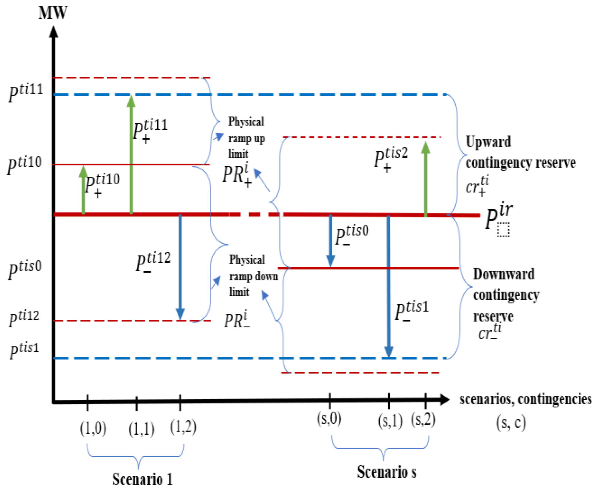
2.3. Load-Following Reserve Ramping under Uncertainty Using ‘Central Path’

In normal conditions, ramping feasibility is only enforced on this high-probability ‘central path’ (Blue colored), as shown in Figure 5, in which all possible transitions are constrained to be feasible with respect to the physical ramping capabilities of generators as well as any load-following reserve capacity. For a high-probability central path, transitions from a small set of base scenarios in one period to a small set of base scenarios in the next period are described by a transition probability matrix.
A simple “wear and tear” cost is defined for load-following reserve/contingency reserve dispatch from one period to another, applied as a probability-weighted cost to each possible transition, as well as ramp-up and ramp-down load-following ramping reserve costs. These reserve costs apply to maximum upward and downward transitions included in the central path scenarios, as illustrated in Figure 5.

2.4. Contingency Condition Reserve Ramping during Uncertainty

In the proposed SSCED problem, as shown in Figure 6, the uncertainty of generation from renewables is modeled as generation scenarios s = 1, s = 2, using transition probability matrices. The reserves are defined by the maximum redispatch deviations across all uncertain generation scenarios and contingencies having the physical ramp rates limit as P R + i and ( P R i ) . The maximum upward deviations ( c r + t i ) and downward deviations c r t i of contingency reserves in contingency cases (c = 1,2….) from the base case within each scenario (s) at time instant t is given by   P t i s 1 , P + t i s 2 ,   etc., as seen in Figure 6.
For the multiperiod problems, the reserve structure is as shown in Figure 6; the variables include a t index as well since the same structure is used at each period t in the multiperiod problems.

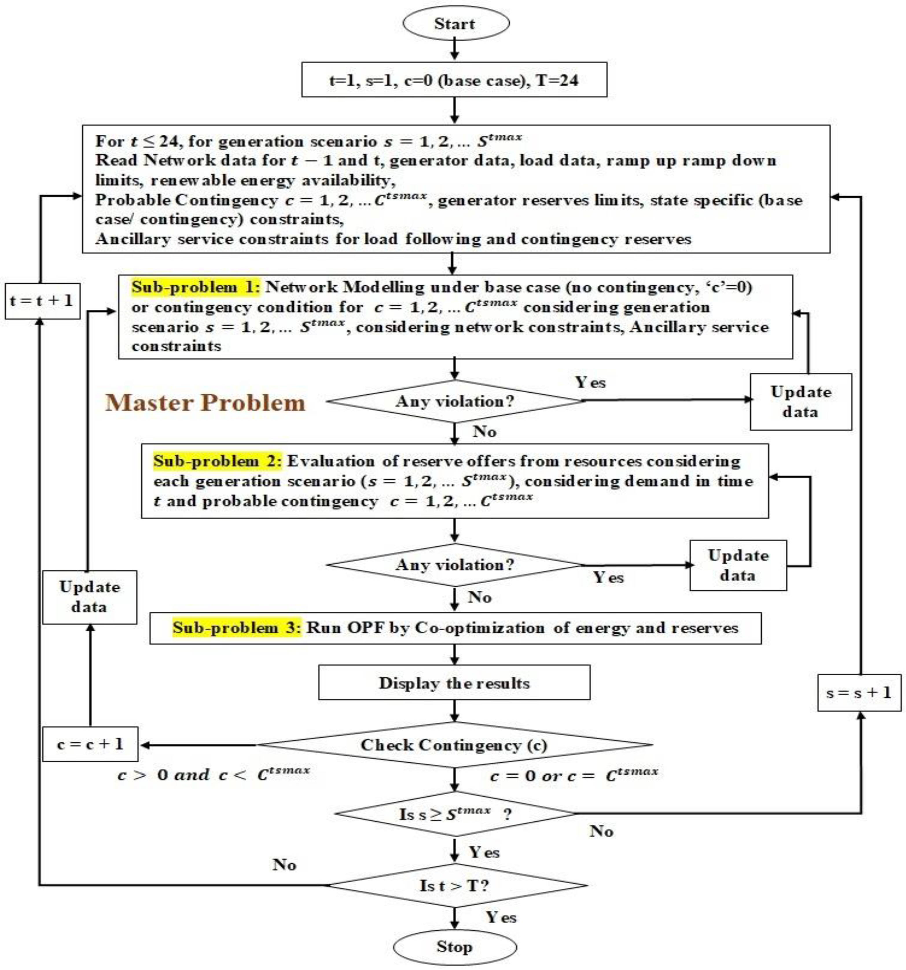
3. Proposed Methodology for Solving Multiperiod SSCED Problem

3.1. Proposed Methodology for Solving SSCED considering the Uncertainty of Renewable Generation and the Uncertainty of Contingency Occurrence

The problem structure is solved using the proposed methodology for SSCED. This methodology follows the procedure shown in the flowchart in Figure 7.
The flowchart in Figure 7 shows the methodology proposed for multiperiod stochastic security-constrained economic dispatch, for a 24 h time period.
The flowchart shows that first, for the base case (without contingency), the initialization of time period t = 1, generation scenario s = 1, and as there is no contingency, i.e., c = 0 is carried out.
All network data are read as it includes generator data, generator ramping limits, renewable energy generation profiles, contingency data (if any), associated generation cost data, and reserve cost data. Then, system data are read for t < 24, and the initial base case probability for each generation profile (scenario) is set to 1. The maximum time period (T) of analysis considered in this work is T = 24. The maximum number of generation scenarios ( S t m a x ) in time period t of the analysis are initialized, the maximum number of probable contingencies in time period t and scenario s is C t s m a x is initialized. This methodology is based on solving the master problem, solved at each time step t.
The Master problem consists of three sub-problems.
The three subproblems are as follows:
Sub-problem 1: Network modeling.
Sub-problem 2: The evaluation of the reserve offer from resources considering the uncertainty of generation scenarios and probable contingency.
Sub-problem 3: Objective function cost minimization by OPF Co-optimization of energy and reserves.
Initially, the energy and reserve dispatch are executed using the “master problem” for base cases (c = 0) in each generation scenario in time period t until s S t m a x . The results are displayed for time period t, and the contingency condition is checked. If there is no contingency, c = 0, and generation scenarios are s > 1, then the generation scenario counter is incremented as s = s + 1 and the process repeats until s S t m a x , i.e., the generation scenario number s becomes greater than, or equal to S t m a x ,   the maximum generation scenario S t m a x in time period t.
In this work, for the stochastic approach using more than one generation profile, i.e., s > 1 is considered. In stochastic security-constrained OPF, for the co-optimization of energy and reserves, the probabilistic contingencies are also considered. The contingency counter is greater than 0 (C > 0), and with multiple generation scenarios, the scenario counter s is also greater than 1 (i.e., s > 1). The maximum number of contingencies in a single time period t and generation scenario s is of analysis C t s m a x .
In subproblem 1, network modeling is carried out as described in Section 3.2. In this subproblem, the cost model for active power from conventional sources is carried out using Equation (1). Equation (2) gives the output from a WECS and its active power cost model is given in Equations (3) and (4). The uncertainty of renewable energy generation scenarios from one period to the next period is modeled by “probability transition scenarios” given by the “probability transition matrix” [16] in Equation (5). The approximation of uncertainty of the state of the system, i.e., the base case or state of contingency, is defined using Equations (6)–(9). If there are any violations, the data are updated so that the state of the system can be decided. The subproblem is executed with the updated data until there are no violations. The program then proceeds further to subproblem 2, for ramping evaluation. In this subproblem, the ramping reserve considers generation scenario s and contingency c, c = 0, for the base case (normal case) and c > 0 for a contingency case. For a high-probability central path, transitions from base scenarios in one period to base scenarios in the next period are given in Equation (10) to Equation (14) for load-following reserves. If the state of the system in the subproblem is a contingency state, then the maximum upward and downward contingency reserve is as explained in Equations (15) and (16), and the amount of the contingency reserve constraints are given in Equations (17) and (18).
After modeling the system in subproblem 1, subproblem 2 is executed as explained in detail in Section 3.3. The ramping evaluation is executed considering the central path and various generation scenarios present in the problem formulation data. In subproblem 2, the ramping reserve requirement in the base case or contingency case is calculated. At each time period t, the ramping reserve requirement corresponds to the reserve quantity, which is calculated based on the demand to be satisfied and the available generation from resources. In a normal state (base case), the load-following reserves are subject to constraints given by Equations (10) and (11). the load-following ramp-up and ramp-down reserves are estimated using Equations (13) and (14).
The contingency reserves ramping constraints given in (15) and (16) are followed while injecting the contingency condition ramping reserves. The ramping limits on transitions from base to contingency cases are given in Equations (17) and (18). If there are any violations in the constraints, then the system data are updated and the loop is again executed until the ramping evaluation is properly executed.
Then, subproblem 3, is executed. This subproblem is discussed in detail in Section 3.4. In this subproblem, the execution of OPF by the co-optimization of energy and reserves is carried out. The objective function is stochastic security-constrained economic dispatch, with a minimization of the total cost of energy and reserves, as given in Equation (19). In the equation for normal operating conditions, i.e., the base case having no contingency, the objective function is as given in Equation (20), and in contingency conditions, the objective function is as given in Equation (21). The objective function in Equation (19) consists of five terms. Each of the terms is executed, as given in Equations (22)–(26), and are
  • The optimization of the expected cost of active power dispatch and redispatch.
  • The optimization of the expected cost of load-following ramping (wear and tear).
  • The optimization of the cost of load-following ramp reserves.
  • The cost of endogenous contingency reserves.
  • The optimization of no-load, startup, and shutdown costs.
These terms in the objective function are subject to network constraints given in Equations (27) and (28), the unit commitment schedule in Equation (29), startup and shutdown events, as explained in Equations (30)–(32), and minimum uptime and minimum downtime constraints, which are explained in Equations (33)–(35). The OPF results are displayed giving the economic dispatch results for energy and reserves, considering the uncertainty of the generation profile and the contingencies.
When the three subproblems have been executed, the contingency for scenario 1 is checked; if the contingency number is less than the maximum contingency, i.e., c < C t s m a x , then the contingency number c is incremented by 1, i.e., c = c + 1, and then the data are updated. This updated data are utilized for executing the three subproblems and again the results are displayed considering contingency no. 2. This process continues until all of the contingencies for scenario 1 are addressed and the contingency counter c is equal to the maximum number of contingencies C t s m a x in scenario s, i.e., c = C t s m a x . If there is more than 1 generation profile, the scenario counter is incremented by 1, i.e., s = s + 1. The data are read considering generation profile no. 2 and the three subproblems are then executed. The program remains in the loop until all contingencies and dispatch decisions are displayed for scenario 2. The flowchart is generalized for the maximum number of scenarios S t m a x . Thus, the master problem is executed considering all contingencies for each generation scenario until s   S t m a x , for the time period t. Once s S t m a x , the time period t is then incremented by 1, i.e., t = t + 1, and again, the data are read for the next time period and the loop continues to be executed until t = 24.

3.2. Subproblem 1: Network Modeling

In subproblem 1, network modeling is carried out. At each time step, as the system data are read, the available generator, its energy and reserve output, load as well as network data are updated. At each time step t, the generation and demand balance are evaluated considering the limitations on the power flow lines and DC power flow constraints. The modeling of active power output from CHP-based generators and active power from WECS output is carried out, as discussed in Section 3.2.1 and Section 3.2.2. The cost of active power from these generators is taken into consideration. Modeling of the uncertainty of active power generation from WECS is carried out by probability-weighted scenarios, as discussed in Section 3.2.3, and the mathematical modeling of the probabilistic transition of states from the base case to the contingency state is carried out, as explained and discussed further in Section 3.2.4.

3.2.1. Cost of Active Power from CHP-Based Generators

The function of the total fuel cost for CHP-based generators ($/h), such as natural gas-based and biogas-based generators in the system, can be presented as a second-order quadratic polynomial, as follows [17]:
C P i j = i = 1 I a + b P i + c P i 2 · $ / h
where C P i j is the cost of active power production from the generator, i is the maximum number of generators, a ($), b (MW), and c ($/MW2) are cost coefficients of the active power production function, and P i j   is the active power produced in MW by generator i at bus j.

3.2.2. Cost of Wind Energy Conversion System (WECS)

The wind turbine’s output power and wind speed are related to the wind energy conversion system, as given in Equation (2). The wind speed is monitored every 10 m in height.
The following equation [18,19] can be used to express how the output power of a wind energy conversion system (WECS) relates to other factors:
P t w = 0 , W w < W c i n W w W c i n W N o r W c i n P t w r a t e d , W c i n     W w     W N o r P t w r a t e d , W N o r     W w     W C O 0 , W w     W C O
where P t w is the wind turbine output in MW at an instant (t), actual wind speed is W w in m/s, P t w r a t e d is the rated power of the WECS, W c i n , W N o r , and W C O are the cut-in speed, rated speed, and cut-out speed, respectively.
The active power cost from the WECS consists of the following cost components
w C w   P t w = w C w , c c + C w , o p P t w + C w , d p   $ / h
where C w , P P t w = the cost function of active power from the WECS in ($/h);
C w , c c = the capital cost ($/MWh); C w , o p = the operation and maintenance cost ($/MWh); C w , d p   = the depreciation cost of the wind turbine w ($/h).
For the wind turbine used in this analysis, the resource i = w
For uncertainty modeling, two wind profiles are considered for the system under study, as shown in Figure 8. Uncertainty modeling for wind power output scenarios by probability-weighted scenarios is discussed further in Section 3.2.3.

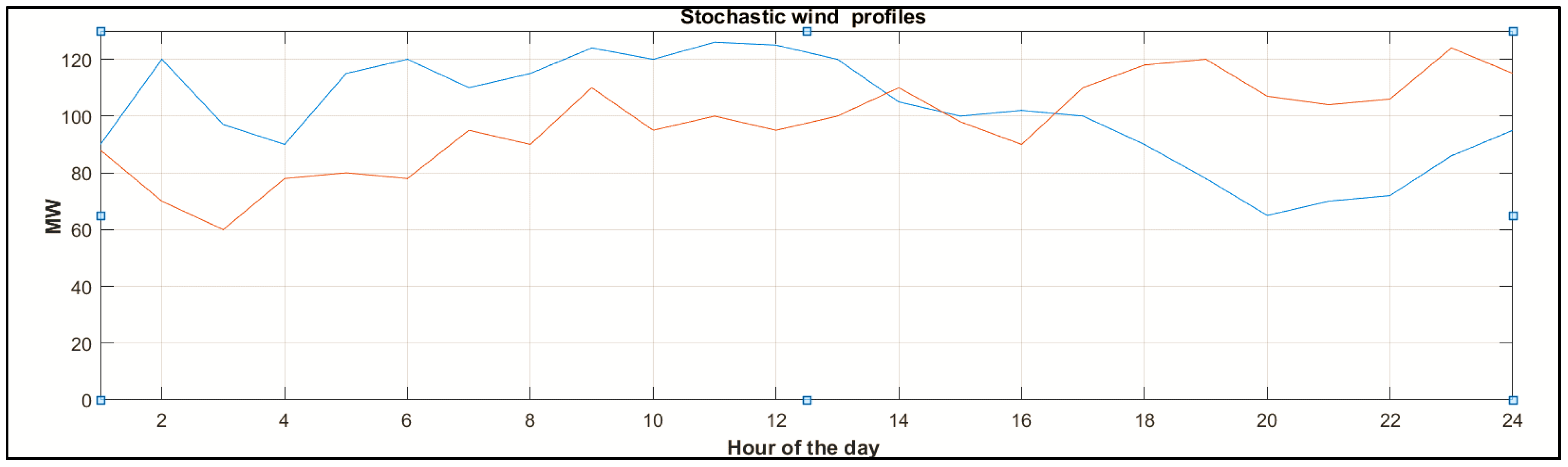
3.2.3. Modeling the Uncertainty of Wind Power Output Scenarios Using Probability-Weighted Scenarios

In this study, the joint distribution of uncertain parameters is used to generate scenarios that are then added to the problem structure as “multiple probability-weighted” [15] base cases to describe the uncertainty of wind power generation. Utilizing “probability matrices”, as shown in Equation (5), with the full transition of generating scenarios, when periods of transition between low, average, and high-probability wind scenarios are permitted, the more general instance of SSCED can be accomplished.
Φ t = ϕ t 11 ϕ t 12 ϕ t 1 n S t 1 ϕ t 21 ϕ t 22 ϕ t 2 n S t 1 ϕ t n S t 1 ϕ t n S t 2 ϕ t n s t n S t 1
Here, in the stochastic model with multiple base scenarios per period, the transition matrix is a cell array of length n t   containing the transition probability matrices Φ t of (5). That is, transmat{t} contains the n S t × n S t 1 matrix of transition probabilities from period t 1 to period t . The first element of the transmat matrix is a column vector of transition probabilities from period 0, ( n S t = 1) to period 1. The columns of Φ t sum to 1 and its coefficients are used to weight the wear and tear costs of ramping for load-following reserves and contingency reserves [13,14,15].

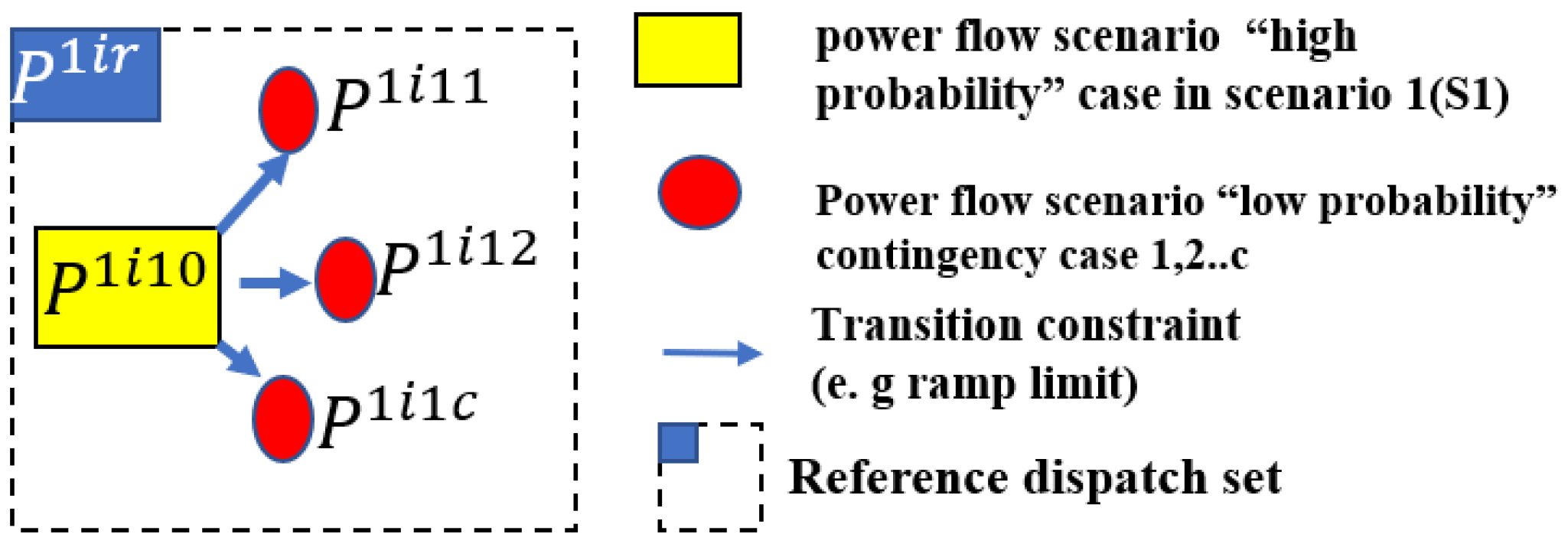
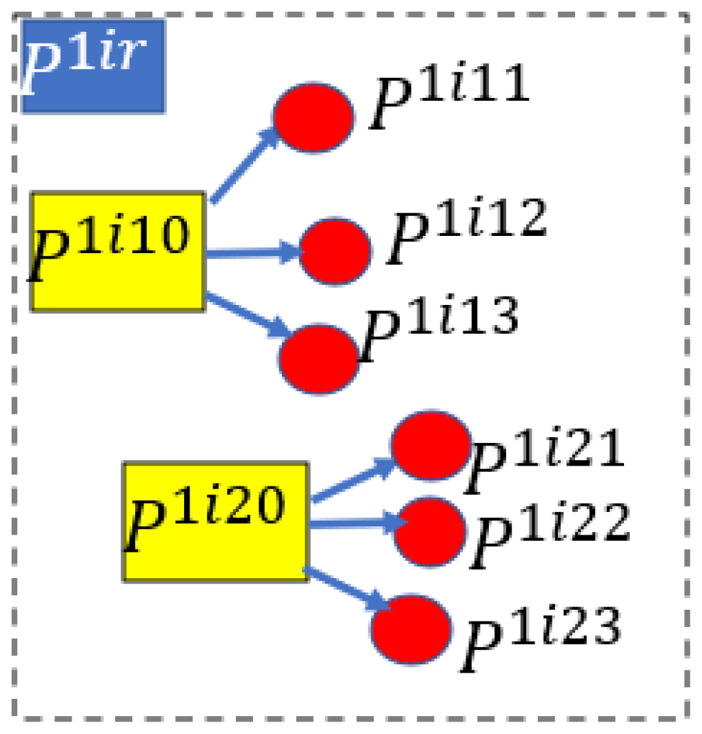
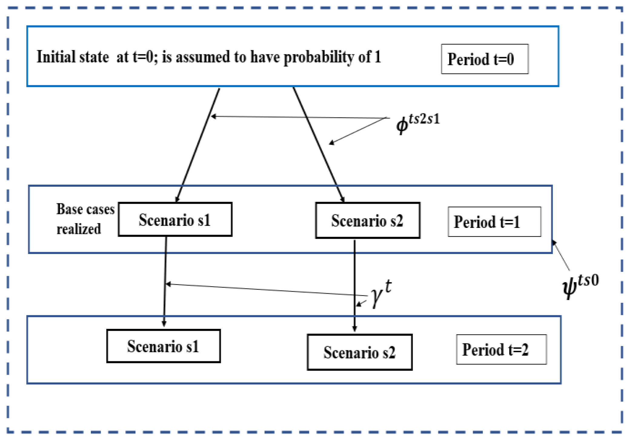
3.2.4. Mathematical Modeling of Probabilistic Transition of States from Base Case to Contingency State [16,20]

The individual state, i.e., scenario-based state and contingency state, is defined by state-specific probabilities ψ t s c for period t, and can be derived from those in period t 1 in two steps [16].
Step 1: Determine the probability γ t s that scenario s for s = 1, s = 2, etc., or any of its aforementioned contingencies will take place at a time t by using the formula
γ t 1 γ t 2 γ t n S t =   Φ t ψ t 1 10 ψ t 1 20 ψ t 1 n S t 1 0
where
γ t s = c C t s ψ t s c                
Step 2: Since the sum of conditional probabilities ψ 0 t s c of contingencies c is 1, we simply scale each by the corresponding γ t s   to obtain the correct state-specific probabilities
ψ t s c = γ t s   ψ 0 t s c      
γ t     s S t 1 ψ   t 1 s 0 = s S t , c C t s ψ t s c < 1 ,   t > 1
The probability of transitioning to scenario s = 2 in period t given that scenario s = 1 was realized in period t 1 is assumed to be a known value ϕ t s 1 s 2 .
In this work, the transition can be explained, as shown in Figure 9. For multiperiod problem structures with contingencies, it is assumed that each period starts from the initial state of t = 0. The initial phase has a probability equal to 1. For period t, the base case according to renewable generation scenarios s = 1, s = 2 with probability Φ t s 2 s 1 and the probability of being in a base case state for each generation scenario without a contingency state is the probability of ψ t s 0 . Scenario 1 and scenario 2, in the system, might transit to any of a number of states in period t + 1 with probability γ t . There are two types of uncertainty considered in this proposed problem structure—contingencies and parameter uncertainty (stochastic renewable energy generation). For this a multistage decision approach with scenario recombination and scenario trimming is considered to avoid the exploding number of scenarios.
As seen in Figure 9, the base case scenario to contingency states in period (t = 2) depends on transition probabilities. Additionally, the transition from base to contingency states, i.e., state-specific probabilities are used to model the probabilistic contingency occurrence.

3.3. Subproblem 2: Ramping Evaluation

In this subproblem 2 of the proposed master problem of SSCED, the reserves are defined by the maximum redispatch deviations across all scenarios and contingencies and the physical ramp rates limit. At each time period t, the ramping reserve requirement corresponds to reserve quantity, which is calculated based on the demand to be satisfied and available generation from CHP generators, its ramping capacity, and the ramping flexibility offered [21,22] by WECS considering its uncertainty.

3.3.1. Mathematical Modeling of Load-Following Ramping Reserves in Normal (Base Case-No Contingency) State

To minimize the mismatch between generation and demand in normal (base case) conditions, the ramp-up ( δ + t i ) and ramp-down ( δ t i ) of the ramping units is subjected to respective ramp-up and ramp-down constraints, as given in Equations (10) and (11) [16].
0   δ + t i
0   δ t i
In normal conditions, the load-following up ( δ + t i )   /down ( δ t i ) ramping reserves are injected. The load-following ramp reserve definition is given in Equations (13) and (14) [16].
Load-following ramp reserve definition:
  t T ,   i I t s c ,   s 1 S t 1 ,   s 2   S t   | ζ t s 2 s 1 = 1
P t 1 i s 1 0 P t i s 2 0     δ t 1 i
P t i s 2 0 P t 1 i s 1 0     δ + t 1 i
The ramping reserves wear and tear costs are defined as a simple quadratic “wear and tear” cost from the difference in a dispatch from one period to another, applied as a probability-weighted cost to each possible transition, as given in Equation (5), as well as up and down load-following ramping reserve costs. These reserve costs apply to maximum upward and downward transitions included in the central path scenarios.

3.3.2. Mathematical Modeling of Contingency Reserves Ramping in Contingency

There are now two types of uncertainty, contingencies and parameter. The reference power dispatch and reserve dispatch decisions from each generator are made before the uncertainty is realized, but the base case or contingency state specific dispatch decisions are based on the type of uncertainty. The contingency reserves ramping constraints are given in Equations (15) and (16) and are followed for injecting the ramping reserves in contingency conditions. The total ramping service provided by all generators is equal to the ramping required by the demand. The ramp-up and ramp-down will be such that it will be the maximum ramping that can take place according to the full transition probabilities-enabled central path, as described in Equations (17) and (18) [16,20].
  • Reserve, redispatch, and contract variables:
0     P + t i s c     c r + t i     c r m a x + t i          
0     P t i s c     c r t i       c r m a x t i      
  • Ramping limits on transitions from base to contingency cases:
P   t i s c   P r t i = P + t i s c P t i s c        
P R i     P t i s c P t i s 0     P R + i ,         c   0

3.4. Subproblem 3: Objective Function Cost Minimization by OPF Co-Optimization of Energy and Reserves

OPF by Co-optimization of energy and reserves is executed in this subproblem. The following objective function is considered in this subproblem.
Objective function: multiperiod stochastic security-constrained economic dispatch of energy and reserves has the following objective function f x for the minimization of the total cost of energy and reserves comprising five components, as given in Equation (19) [16]
min f x = f P P ,   P + ,   P + f δ P + f l f δ + ,   δ + f c r c r + ,   c r + f s u ,   v ,   w
where f x   is comprised five components, and consideration of each component depends upon the normal state or contingency state of the system. The first term is generators active power dispatch and redispatch cost, the second term is load-following ramping wear and tear cost, the third term is expected load-following ramp reserve cost, the fourth term is endogenous contingency reserve cost (optional), and the fifth term (last term) is a startup and shutdown cost.
  • In the normal state, the objective function becomes:
min f x = f P P ,   P + ,   P + f δ P + f l f δ + ,   δ + f s u ,   v ,   w
  • In the contingency state, the objective function considered is as follows:
min f x = f P P ,   P + ,   P + f c r c r + ,   c r + f s u ,   v ,   w
Each of the five components is expressed in terms of the individual optimization variables as follows.
1.
Optimization of the expected cost of active power dispatch and redispatch ($/h)
f P P ,   P + ,   P = t T s S t c C t s ψ α t s c i I t s c C P t i   P t i s c + C P + t i P + t i s c + C P t i P t i s c
where C P t i   P t i s c is the cost function for active power injected by unit i at time t. C P + t i P + t i s c is the cost function for upward deviation from the reference active power. C P t i P t i s c is the cost function for downward deviation from the reference active power quantity for unit i at time t for scenario s and contingency c.
2.
Optimization of the expected cost of load-following ramping (wear and tear) ($/h)
f δ P = t T γ t s 1 S t 1 s 2 S t ϕ t s 2 s 1 i I t s 2 0 C δ i P t i s 2 0 P t 1 i s 1 0   $ / h
In the above equation, C δ i gives the ramping cost for a time period (t), of unit i, when the system is in the normal state, i.e., contingency c = 0, and there is a transition of the system from scenario 1 (s1) in time period (t − 1) to scenario 2 (s2) in time period t.
Ramping reserves are procured on the difference between the dispatches for adjacent periods (t − 1) having scenario 1, to a period (t) having scenario 2.
3.
Optimization of cost of load-following ramp reserves ($/h)
f l f δ + ,   δ = t T γ t i I t C δ + t i   δ + t i + C δ t i   δ t i $ / h
where,
C δ + t i is the cost of upward load-following ramp reserve for unit i at time t for transition to time t + 1 in $/MWh.
δ + t i is the upward load-following ramp reserve in MW.
C δ t i is the cost of downward load-following ramp reserve for unit i at time t for transition to time t + 1 in $/MWh.
δ t i is the downward load-following ramp reserve in MW.
4.
Cost of endogenous contingency reserves in ($/h)
f c r c r + ,   c r = t T γ t i I t C R + t i   c r + t i + C R t i c r t i $ / h
where,
C a c + t i   c r + t i = the cost function for the upward contingency reserves purchased from unit i at time t in $/h.
C a c t i c r t i = the cost function of the downward contingency reserve purchased from unit i at time t.
5.
Optimization of no-load, startup, and shutdown costs in ($/h)
f s u ,   v ,   w = t T γ t i I t C P t i   0   u t i + C v t i v t i + C w t i w t i   $ / h
where,
C P t i   0   u t i = the no-load cost function for unit i time t in $ per startup/shutdown.
C v t i   v t i = the shutdown cost function for unit i time t in $ per startup/shutdown.
C w t i   w t i = the shutdown cost function for unit i time t in $ per startup/shutdown.
This objective function is to be satisfied at each time step for multiple periods under consideration for analysis, modeled as discussed.
While running the OPF, the objective function is exposed to multiple generating units and network constraints. Uncertainty modeling is carried out in this subproblem to model various generation scenarios created by probabilistic-weighted functions, as given in Equation (5), and probabilistic endogenous contingency events, as given in Equation (6).
  • Network operations Constraints:
The objective function in Equations (19) and (20) is subject to the following network constraints for all t T , all s S t , all c C t s , and all   i I t s c , beginning with the constraints that are separable by period.
Power balance equations:
θ t s c ,   V t s c ,   P t s c = 0
Power flow limits, voltage limits, and any other OPF inequality constraints:
θ t s c ,   V t s c ,   P t s c   0
  • Unit Commitment:
For stochastic problems modeling multiple scenarios and/or contingency states, there is a single commitment schedule shared by all states. That is, in the current formulation, a single binary variable is used to model the commitment for a given unit across all scenarios and contingencies in a given period.
  • Generator injection limits and commitments:
u t i P m i n t i s c     P t i s c     u t i P m a x t i s c
  • Startup and shutdown events:
u t i u t 1 i = v t i w t i                  
0     v t i       1            
0     w t i       1      
  • Minimum up and down times:
y = t T i + 1 t v y i u t i              
y = t T i + + 1 t w y i 1 u t i                
u t i = { 0 , 1 }

4. Case Study and Results

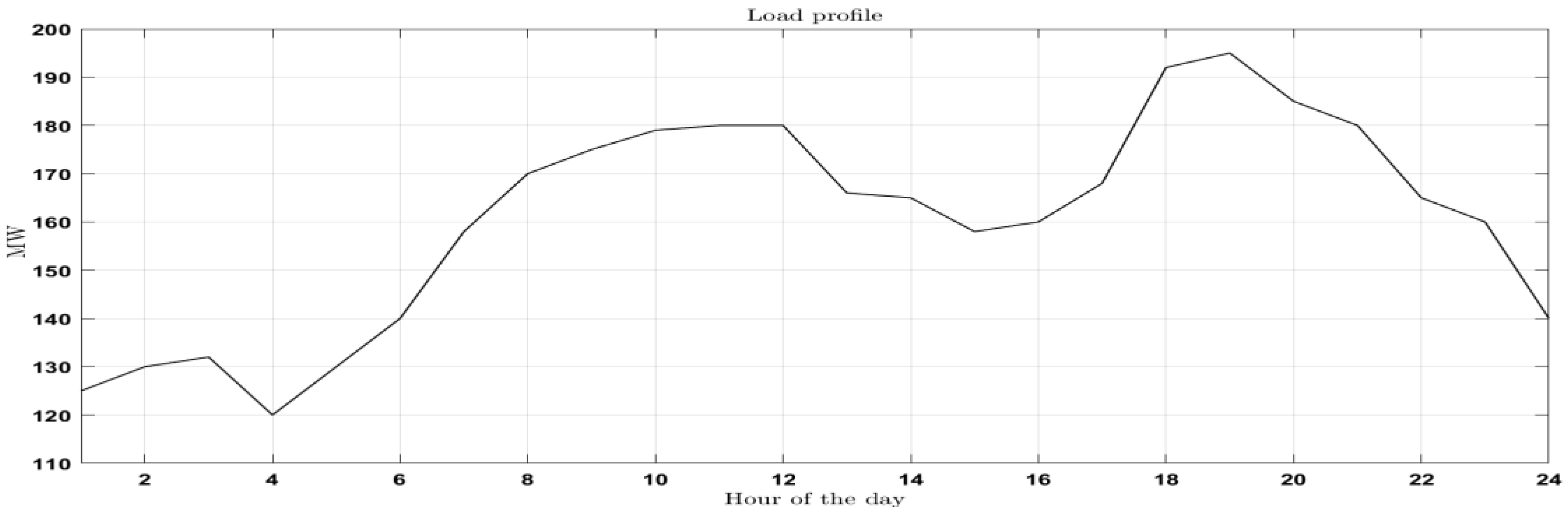
4.1. System Configuration

The modified “IEEE 30 Bus system” [23,24] is considered for the implementation of the proposed SSCED. The grid-connected microgrid is assumed to have a natural gas-based plant at the slack bus, a local CHP-based biogas generation system, and 1-WECS. The data for the generators is given in Table 1. The schematic of the system is shown in Figure 10. For creating the uncertainty of renewable generation, two wind energy profiles [25] are considered for analysis, as shown in Figure 9. These profiles are obtained using predicted wind profiles in Pune, India. The W c i n is the cut-in velocity = 12 km/h, W C O is the cut-out velocity = 90 km/h, W N o r is the normal velocity at that instant, and W w is the wind speed. The conversion efficiency is considered as 90%.
The typical load profile is shown in Figure 11.
Figure 11. Typical load profile for Pune, India [26].
Energies 16 02607 g011
Table 1. Data for generators.
Bus NumberGenerator Type (Fuel)Pmax
Pmin
$/MWRamping Capability [27]Contingency Reserve
Positive and Negative Active Reserve in MW
1Natural gas80 90±5 to 8%±10
10
2WECS (Wind 1)10030±30–60%±30
20
27Biogas Gen 15580±8 to 10%±10
10
22Biogas Gen 25080±8 to 10%±10
10
23Biogas Gen 33080±8 to 10%±10
10
13Biogas Gen 44080±8 to 10%±10
10

4.2. Case Studies

  • Case 1: Base case—Normal State (load-following ramping reserve ancillary service)
  • Case 2: Contingency condition—Generator outage occurrence in Case 1, contingency reserve ancillary service
  • Case 3: Contingency condition—Underloading for 24 h (load decreased by 20% for all 24 h) of Case 1, contingency reserve ancillary service.
    These case studies are executed using Matpower Optimal Scheduling Tool (MOST) [16].
Assumptions:
  • The voltages of DG units and PCC change.
  • In the range of (5%), i.e., 95% to 105% of the rated value.
  • All conventional and distributed energy sources have P/f droop control capability.
  • Well-equipped communication infrastructure is present in grid-connected microgrids.
  • The timescale considered for load-following ramp-up and ramp-down services reserves is 1 h for the simplicity of analysis.
  • The frequency of the system is maintained at 50 Hz with ±0.5 Hz tolerance.

4.3. Results and Discussion

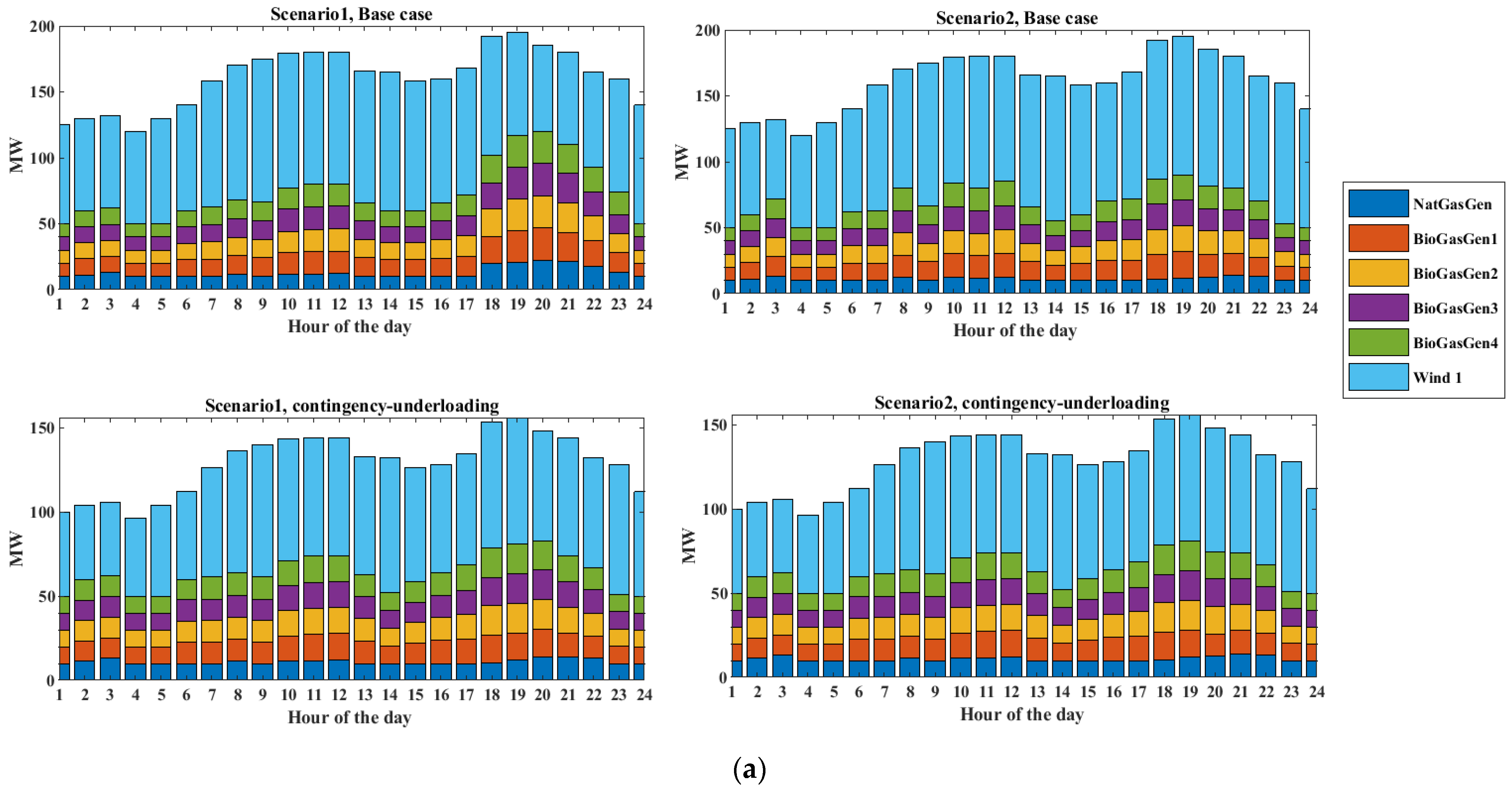
4.3.1. Case 1: Base Case—Normal State: Load-Following Ramping Reserve Ancillary Service

Power Generation in Case 1

After the execution of the master problem, the power generation obtained in the normal state of the system from all six generators including the WECS (Wind1) is shown in Figure 12. The uncertainty of the renewable energy output, i.e., stochastic wind energy generation, has two stochastic wind profiles and is modeled using probability-weighted scenarios. The scenarios are actuated such that the probability of transition of the output from WECS for scenario 1 of the generation profile is 0.1 and for scenario 2 of the generation profile is 0.8. The power generated considering the two generation profiles with the transition as per the transition probability values is shown in Figure 12.
In normal conditions, for each ramping process in load-following, the wear and tear cost is considered from Equation (23), the cost of load-following ramping reserves is taken into consideration, as given in Equation (24), the constraint followed for load-following reserve is as per Equations (10) and (11), and the amount of load-following reserves is estimated by Equations (13) and (14).
The results obtained by the execution of proposed subproblem 2 of the master problem of SSCED are plotted in Figure 13a, showing the ramp-up reserves, and Figure 13b, showing the ramp-up reserve price. Similarly, Figure 13c shows the ramp-down reserves and Figure 13d shows the ramp-down reserve price, which is mainly due to the wear and tear costs associated with each load-following ramping.
As seen in Figure 13a, the ramping reserves follow the full transitions central path, which injects the high-probability ramping reserves from the WECS and other sources. The maximum ramp-up and ramp-down occur as per Equations (13) and (14).

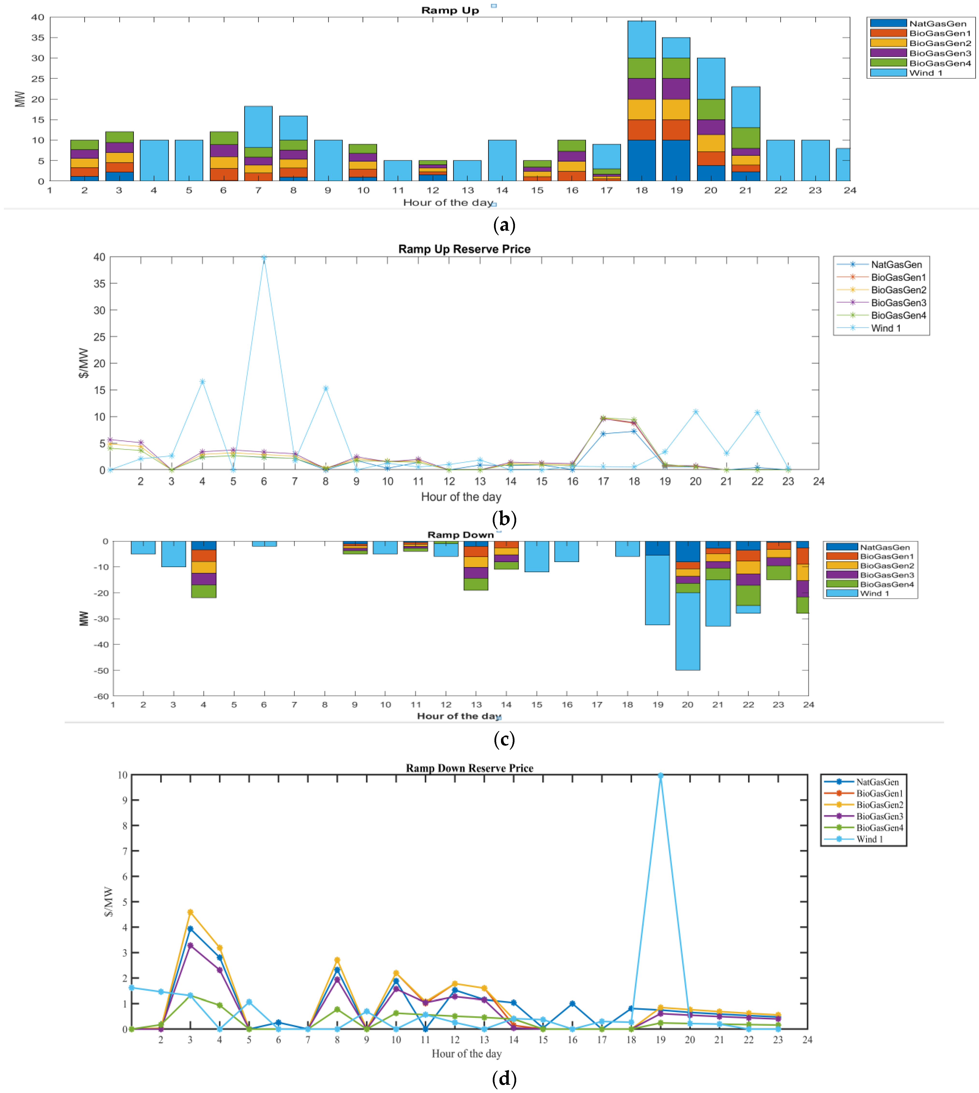
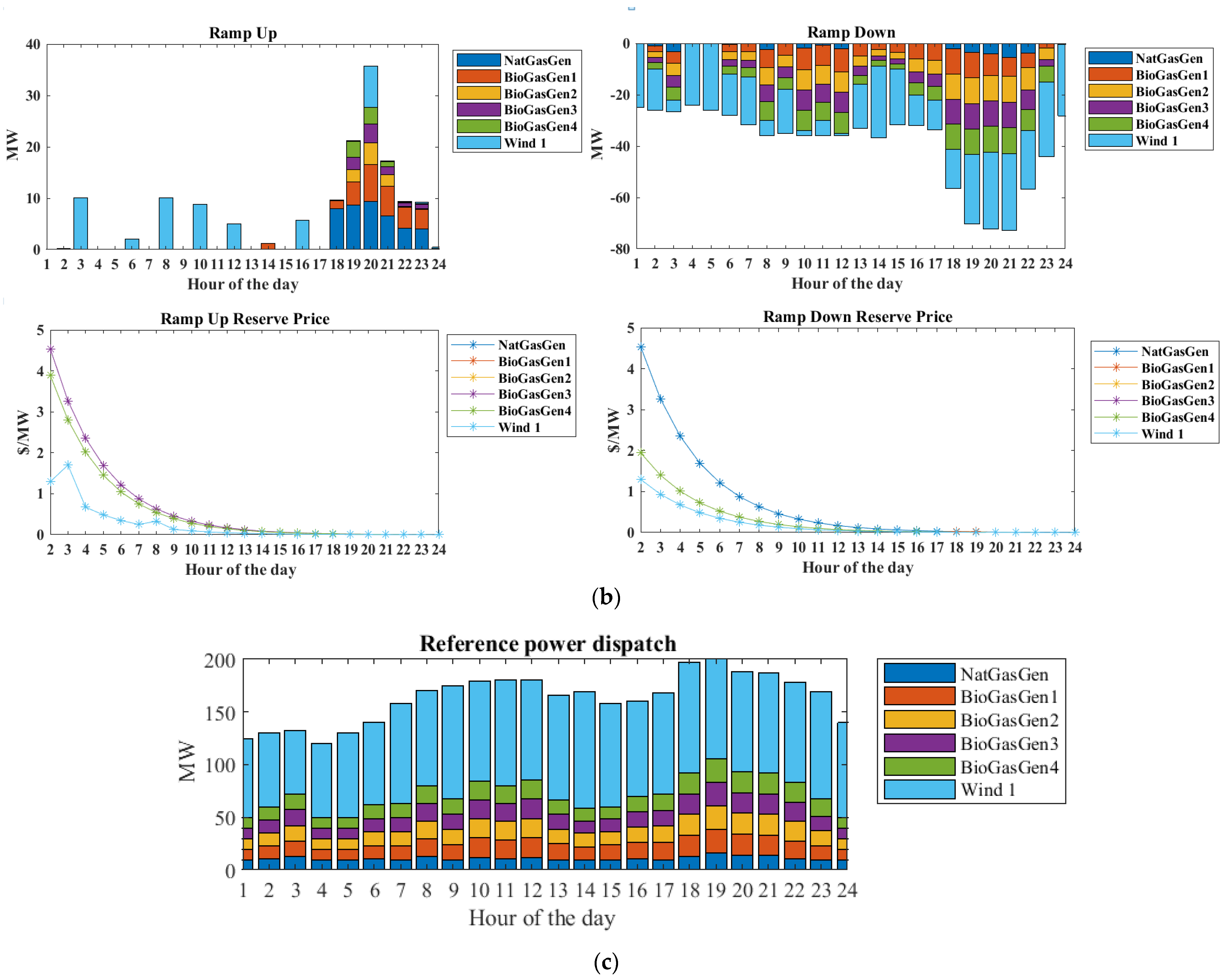
Ramping Process in Case 1: Normal Condition (Base Case)

In normal conditions (base case), the load-following ramping can be explained in detail for each time period. For example, the load-following ramping process is explained considering the ramping period t = 3rd hour, and observed from Figure 13a,b, at period (t − 1) = 2nd hour and period t + 1 = 4th hour. As discussed earlier, the ramping up/down of generators in time period t for unit i for transition to the time period t + 1 from period t depends upon the power generated in time period (t − 1). Here, t = 3 if natural gas generator i = 1, the power generated in the base case in (t − 1) period = P 3 1 110 = 11.18 MW. The power produced in scenario 2 in time period t = 3, i.e., P 3120 is 13.38 MW. This natural gas generator ramps up by 2.19 MW in period t. A similar dispatch takes place for biogas generators no. 1, 2, and 3 and biogas generator no.4. For the wind generators (Wind 1), the generated power in period t − 1 is 70 MW in scenario 1, and for scenario 2, it is 60 MW; therefore, it will ramp down by 10 MW, as shown in Figure 13c, and its price is shown in Figure 13d, according to Equations (13) and (14). This procedure is followed for each time step while solving the proposed SSCED master problem according to the updated data and system condition.

Operating Cost Minimization in Case 1: Normal Condition (Base Case)

The proposed SSCED gives the optimized objective function cost of $9819/day. If the flexibility of wind energy is increased from 30% to 40%, the WECS injects power with more ramping capacity, and the overall objective function cost reduces to $9057/day. The operation cost is minimized by almost 8.1%. It is, therefore, observed that the load-following ancillary service is efficiently and economically provided by the WECS, even with having an uncertain nature. By the use of the weighted-probability scenario method, its uncertainty is modeled properly, which is then converted into an advantage.

4.3.2. Case 2: Contingency Condition: Generator Outage Occurrence in Case 1, Contingency Reserve Ancillary Service

In this case, the contingency occurrence is simulated as a generator outage. Biogas generator no. 4, is the outage generator.

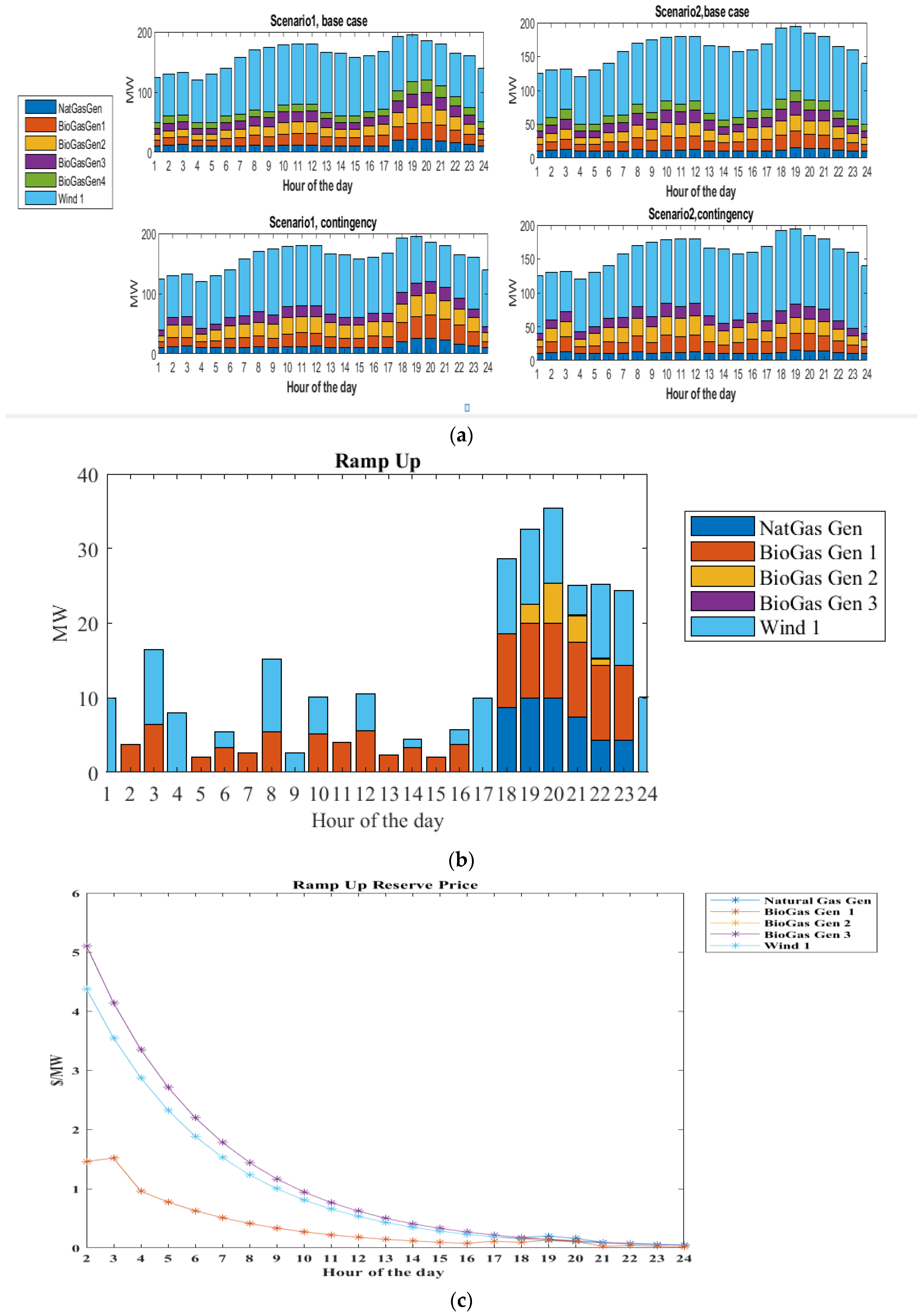
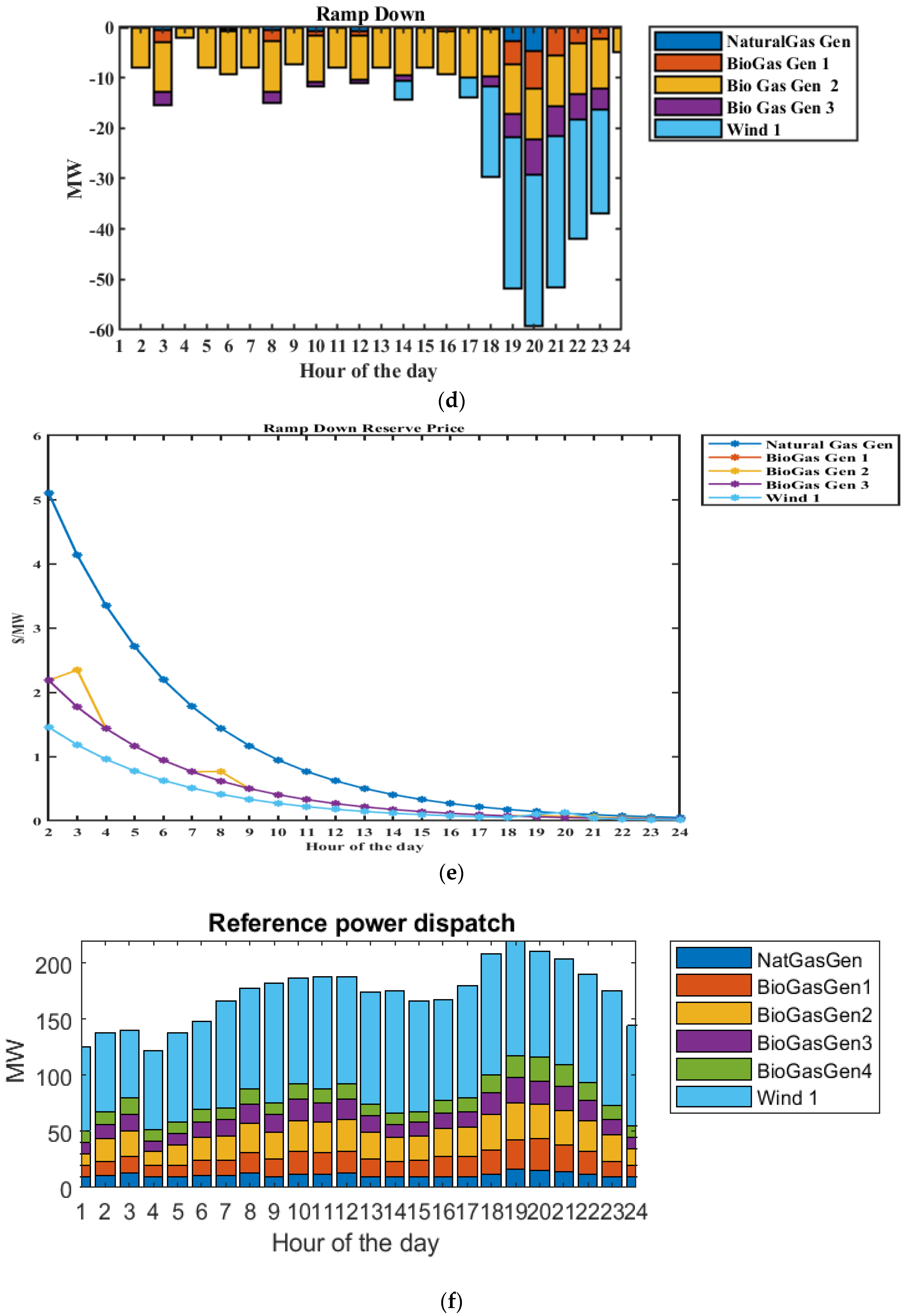
Power Generation in Case 2

SSCED is carried out in case 2 for probabilistic generator outage contingency conditions. This probabilistic contingency is modeled using a probability-weighted scenario and a state-specific probability function, as discussed earlier in subproblem 1.
As seen in Figure 14a, the power generation is shown for scenario 1 for the base case and contingency condition (generator outage-Gen 4), and the power generation for scenario 2, for the base case and contingency condition. Figure 14b shows the ramp-up reserves in MW, the WECS injects maximum ramp-up reserves along with the biogas-based Gen 1, Gen 2, and Gen 3, and helps to cope with the loss in generated power that was offered by biogas generator no.4, which is the outage generator.

Ramping Process in Case 2: Contingency Condition (Generator Outage)

For understanding the SSCED in the contingency condition ramping process in subproblem 2 of the master problem, the ramping at time period t = 3, t − 1 = 3 − 1 = 2, i.e., time period 2 is considered. The two base case scenarios (scenario 1 and scenario 2) are actuated with a probability of transition of 0.1 and 0.8. For contingency cases, the fraction of the time slice is α , that is, the spent in the base case before the contingency occurs ( α = 0 means the entire period is spent in the contingency). The biogas-based generator 4 at bus 13 is in outage from t = 1, for the complete time period, as seen in Figure 14a. The contingency condition is actuated with α = 0 . The network constraints and contingency reserve constraints are followed while offering the contingency reserves, as seen in Figure 14b, with its price in Figure 14c, and maintaining the power supply to the load. Ramping limits on transitions from base to contingency cases follow Equations (15)–(18). As there are two renewable energy generation scenarios considered to model the uncertainty of renewable wind power generation, each generator will ramp-up/down to its maximum to achieve the central path of ramping according to the maximum difference between the power dispatched by that generator in contingency P t i s c   , with the number of contingencies c = 1 and base case scenario P t i s 0 , for scenario 1, and the same procedure will occur for scenario 2 power dispatch during contingency. For time period t = 3, i = 1 for the natural gas generator at bus no.1, in the base case, for generation scenario s = 1, the power produced by natural gas generator 1 = P 3110   = 13.03 MW, and for the contingency condition c = 1, it produces P 3111   = 13.03 MW. For generation scenario s = 2, for same time period t = 3, the power produced by generator number i = 1 in the base case = P 3120   = 1 3.50 MW, and for the contingency condition, c = 1, in the same time period, t = 3, the generated power is P 3121   = 13.50 MW. In this case, in order to get the maximum contingency reserve ramping, the reference dispatch for generator number ‘i = 1’ for natural gas generator, P r 31 is 13.50 MW. Therefore, according to Equation (17), P 3111     P r 31   = −0.47 MW; therefore, the generator will not ramp-up but will ramp down by 0.47 MW. The ramp-down reserve prices are shown in Figure 14e.
It is to be noted that as per the reserve requirement, the generators provide both ramp-up and ramp-down contingency reserve quantities for the same time period t = 3. This can be explained as follows:
For same time period t = 3, for biogas-based generator 2, i = 2, in base case for scenario 1, c = 0, the power produced = P 3210 is 12.3 MW, and for same time period t = 3, for biogas-based generator 2, i = 2 for contingency condition c = 1, P 3211   = 14.72 MW.
For base case scenario 2, for c = 0, the power produced by the same generator is given by P 3220 = 14.72 MW, and for the same scenario, contingency condition c = 1, the power generated is P 3221   = 21.17 MW. Therefore, the maximum difference is observed for scenario s = 2 between the contingency and base case ramping up, i.e., 6.44 MW. The reference active power dispatch value of P r 32 is 14.72 MW, as seen in Figure 14f. This generator, therefore, ramps down at maximum for scenario 1 considering the power difference between probabilistic the contingency and the base case as 2.42 MW. As full trajectories in the transition probabilities are considered, the maximum ramping of reserves takes place. For all other generators, the same ramping process is followed to achieve the generation load balance in event of a loss of one of the generators. The WECS provides the maximum flexible ramping and, hence, is an ideal source for providing contingency spinning reserves. P R + i ,   P R i are the upward/downward physical ramping limits for unit i for transitions from the base case (c = 0) to the contingency cases (c = 1). The upward/downward deviation from the active power (reference) quantity P t r i for unit i in the post-contingency state c of scenario s at time t is P + t i s c ,   P t i s c . The reference dispatch is shown in Figure 14d.

Operating Cost Minimization in Case 2

After running the proposed SSCED successfully, the objective function cost is minimized to $27,622/day. The WECS flexibility to offer reserves is set to 30%. The expected energy cost is predominantly governed by the wind energy system. When the flexibility of the WECS is increased to 40% ramping capability, the minimized objective function cost then becomes $27,605/day. There is a reduction in objective function cost and the expected energy price also reduces.

4.3.3. Case 3: Contingency Condition: Underloading for 24 h (Load Decreased by 20% for All 24 h) of Case 1, Contingency Reserve Ancillary Service

Power Generation in Case 3

During probabilistic underloading contingency conditions, the SSCED is carried out using the transition probabilities and state-specific probability function. Figure 15a shows the power generated in the base case and contingency case for generation scenarios 1 and 2.

Ramping Process in Case 3: Contingency Condition

Figure 15b shows Ramp-up/down reserves injected and their prices during contingency. It shows that the WECS ramps down at its maximum capacity and maintains the system’s stability. Figure 15c shows the reference dispatch utilized as a contingency reserve limit. For understanding security-constrained economic dispatch, in underloading contingency conditions, consider the time period t = 3 h. The load is reduced from 172 MW to 132 MW and the generators ramp-up/down accordingly to fulfill the reduced load. The active power generated by generator 1, i.e., the natural gas generator in the base case for scenario s = 1, P 3110 = 11.42 MW, and the active power generated in the contingency scenario 1 = P 3111   = 10 MW. At the same time period for generator 1 in the base case scenario s = 2, the power generated, P 3120 = 13.25 MW, and for scenario s = 2, the contingency condition, generator 1 will produce P 3121 = 10 MW, so the maximum ramping reserve obtained is in this condition; therefore, the generator will ramp down by 3.25 MW. This procedure is repeated for all generators including the WECS. The reference power dispatch is shown in Figure 15c.
The maximum ramping estimated from (15)–(17), comparing the power generated in base case scenario 1, s = 1, and scenario s = 2 with their respective contingency states, is finally considered for ramping. Furthermore, the constraint of ramping limit in (18) is followed to obtain the final contingency ramp-up ramp-down value.

Operation Cost Minimization in Case 3

Operation costs are $18,623/day with the ramping capability of the WECS. The impact of resource flexibility on objective cost reduction is clearly observed from the results. If the flexibility of the WECS is increased to 40%, the overall objective function cost decreases to $18,598/day. As WECS is a renewable energy- based source, it is cheaper than other sources. Even if the WECS provides greater flexibility, the per-unit ramping reserve cost is less than the ramping reserve cost of other generators.
As observed from all three cases, the proposed SSCED is ideal for OPF with the co-optimization of energy and reserves in normal and contingency conditions considering uncertainty. It is also observed from Table 2 that if the flexibility of the WECS is increased to 40%, then the objective function cost, i.e., the cost of energy and reserves, reduces. Additionally, the system performance is improved in the case of contingencies, as the increased flexible ramping improves the generation load balance considering the low-cost generator, i.e., the WECS.

5. Conclusions

This work attempted to solve the stochastic security-constrained economic dispatch of load-following and contingency reserves ancillary service during uncertainty through the use of a grid-connected microgrid. An attempt was made to model the uncertainty of wind power output and the uncertainty of the probabilistic contingency conditions using “probability-weighted scenarios and transition matrices” [13]. The wind energy source is purposely included in this analysis to demonstrate its capability in providing a flexible ramping reserve.
Its flexibility is advantageous in normal and probable contingency conditions. The results show that there is a reduction in operating costs by increasing flexibility from 30% to 40% with the WECS providing the reserves.
The methodology implemented in each case under study demonstrates the potential technical, economical, and reliability benefits of load-following ramping reserve ancillary service and contingency reserves ancillary service in major contingency, which comes under frequency control ancillary services.
This work can be extended considering energy storage and its ramping capability providing frequency control reserves, enhancing the system performance, and reducing the operation cost drastically, in normal and contingency conditions. It can be incorporated for stochastic modeling in SSCED, considering its losses, state of charge, storage cycle, and all of its constraints.

Author Contributions

Conceptualization, K.M.K. and G.A.V.; methodology, K.M.K. and G.A.V.; software, K.M.K. and G.A.V.; formal analysis, K.M.K. and G.A.V.; investigation, K.M.K.; resources, K.M.K. and G.A.V. data curation, K.M.K. writing—original draft preparation, K.M.K. and G.A.V.; writing—review and editing, K.M.K. and G.A.V.; visualization, K.M.K. All authors have read and agreed to the published version of the manuscript.

Funding

This research received no external funding.

Data Availability Statement

Data available in a publicly accessible repository. The data presented in this study are openly available in [16,20,23,24,25,26,27].

Conflicts of Interest

The authors declare no conflict of interest.

Nomenclature

t Index of time periods (1 h).
TSet of indices of periods in the planning horizon, typically 1   .   .   .   n t = 24   h .
sIndex of scenarios.
S t Indexes of every possible scenario taken into consideration at time t.
S t m a x Maximum number of generation profiles (scenarios) in time period t.
cIndex of post-contingency cases (c = 0 for the base case, meaning that there was no contingency).
C t s m a x Maximum number of contingency indices taken into account in scenario s at time period t.
i Injections index (generation units).
I t Indices of all the units (generators, dispatchable, or curtailable loads) that are available for dispatch in any situation at time t.
P r t i 
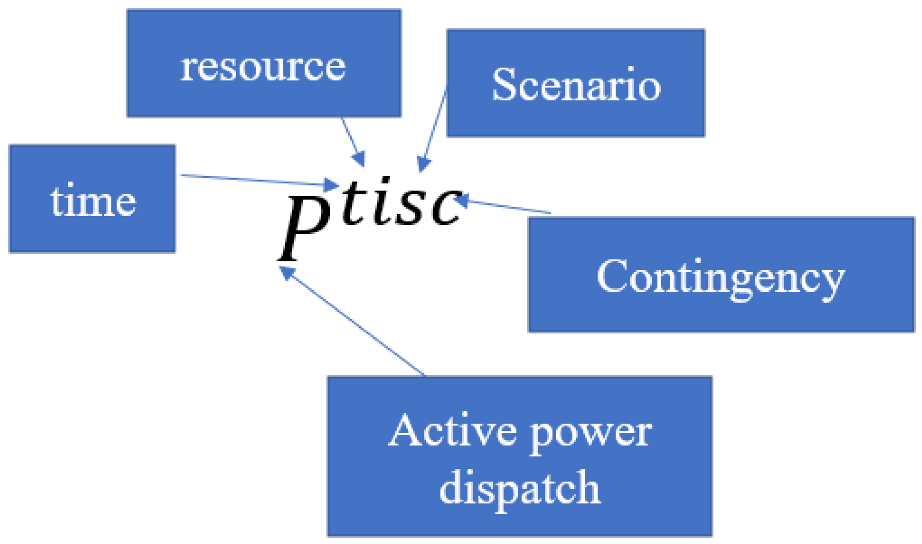
Quantity/reference of the active power dispatching active power to unit I at time t.
c r + t i ,   c r t i Unit i at time t provides an active contingency reserve quantity that is moving upward or downward.
c r m a x + t i ,   c r m a x t i Maximum capacity restrictions for the unit i at time t can go up or down.
P m i n t i s c ,   P m a x t i s c Limits on active injection for unit i at time t in a post-contingency state c of scenario s.
δ + t i ,   δ t i Unit i is required to provide ramping reserves for loads moving up or down for the changeover to time t + 1 at time t.
θ t s c ,   V t s c ,   P t s c Angles and magnitudes of the voltage as well as active injections of power for the post-contingency condition (state c) of scenario (s) at time (t).
δ m a x + t i ,   δ m a x t i Limits for unit i upward/downward load-following ramping reserves at time t for the transition to time t + 1.
    ψ α t s c Probability Contingency k in the scenario s at the time t, adjusted for α .
α For contingency cases, the fraction of the time slice that is spent in the base case before the contingency occurs.
Δ Length of the time slice for scheduling, usually 1 h.
u c t i Binary commitment state: 1 if a unit is online, otherwise 0, for unit i in period t.
ψ 0 t s c Probability conditional on reaching period t without deviating from the main path in a contingency in periods 1…t − 1 and on scenario s being realized in some way of the contingency c in scenario s at period t. (base or contingency). The basic case, or conditional probability of no contingency, is ψ 0 t s 0 .
ϕ t s 2 s 1 Probability of moving from scenario s1 to scenario s2 in period t, given that s1 was completed in period t − 1.
ζ t s 2 s 1 Whether the transition to scenario s2 in Period t, assuming that scenario s1 from period t − 1 should be included in the load-following ramp requirements, is indicated by a binary-valued mask.
  ψ   t s c Estimated likelihood of contingency c in scenario s at time t using transition probabilities ϕ t s 2 s 1 . Conditional probabilities of contingencies ψ 0 t s c .
P R + i ,   P R i Physical ramping upper/lower limits.
for unit i when moving from base (c = 0) to contingency scenarios.
u t i For unit i in period t, the commitment state is binary: 1 if the unit is online, otherwise 0.
v t i ,   w t i For unit I in period t, there are binary startup and shutdown states: 1 if the unit experiences a startup or shutdown event in period t, otherwise 0.
C P t i   · Cost formula for i at time t for active injection.
C P + r i   · ,  
C P r i   ·
Cost for a deviation from the active power reference quantity for unit i at time t in either an upward or downward direction.
C a c + t i   · ,
C a c t i   ·
Cost formula for a contingency reserve that was bought from unit i at time t.
C δ + t i   · ,  
C δ t i   ·
Cost of the ramp reserve for an upward or downward load for unit i at time t for the transition to time t + 1.
C δ i   · On the difference between the dispatches for unit i in neighboring periods, there is a quadratic, symmetric ramping cost.
C ˜ P t i   · With the no-load cost eliminated, the cost function for active power injection has been modified to read as C ˜ P t i   P     C P t i   P C P t i   0 .

References

  1. Chowdhury, S.P.; Chowdhury; Crossley, P. Microgrids and Active Distribution Networks; The Institution of Engineering and Technology: London, UK, 2009. [Google Scholar]
  2. Braun, M. Technological Control Capabilities of Der To Provide Future Ancillary Services. Int. J. Distrib. Energy Resour. 2007, 3, 191–206. [Google Scholar]
  3. Oureilidis, K.; Malamaki, K.N.; Gallos, K.; Tsitsimelis, A.; Dikaiakos, C.; Gkavanoudis, S.; Cvetkovic, M.; Mauricio, J.M.; Maza Ortega, J.M.; Ramos, J.L.M.; et al. Ancillary Services Market Design in Distribution Networks: Review and Identification of Barriers. Energies 2020, 13, 917. [Google Scholar] [CrossRef] [Green Version]
  4. Smeers, Y.; Martin, S.; Aguado, J.A. Co-optimization of Energy and Reserve with Incentives to Wind Generation: Case Study. IEEE Trans. Power Syst. 2022, 37, 2063–2074. [Google Scholar] [CrossRef]
  5. Available online: http://www.forumofregulators.gov.in/data/Reports/SANTULAN-FOR-Report-April2020.pdf (accessed on 2 December 2022).
  6. Shah, C.; Wies, R. Three-stage Power Flow & Flexibility Reserve Co-Optimization for Converter Dominated Distribution Network Lookahead Model using Blockchain & S-ADMM—I: Method. TechRxiv 2022, TechRxiv.11-08-2022. [Google Scholar] [CrossRef]
  7. Ozay, C.; Celiktas, M.S. Stochastic optimization energy and reserve scheduling model application for alaçatı, Turkey. Smart Energy 2021, 3, 100045. [Google Scholar] [CrossRef]
  8. Jin, Y.; Wang, Z.; Jiang, C.; Zhang, Y. Dispatch and bidding strategy of active distribution network in energy and ancillary services market. J. Mod. Power Syst. Clean Energy 2015, 3, 565–572. [Google Scholar] [CrossRef] [Green Version]
  9. Cong, P.; Tang, W.; Zhang, L.; Zhang, B.; Cai, Y. Day-ahead active power scheduling in active distribution network considering renewable energy generation forecast errors. Energies 2017, 10, 1291. [Google Scholar] [CrossRef] [Green Version]
  10. Kurundkar, M.K.; Karve, M.G.; Vaidya, M.G. Comparative performance analysis of Firefly algorithm and Particle swarm Optimization for Profit Maximization of Grid connected Microgrid providing energy and ancillary service. Solid State Technol. 2021, 64, 4610–4626. [Google Scholar]
  11. Ye, H.; Li, Z. Pricing the Ramping Reserve and Capacity Reserve in Real Time Markets. arXiv 2015, arXiv:1512.06050. [Google Scholar]
  12. Fang, X.; Sedzro, K.S.A.; Hodge, B.S.; Zhang, J.; Li, B.; Cui, M. Providing Ramping Service with Wind to Enhance Power System Operational Flexibility; National Renewable Energy Laboratory, University of Texas at Dallas: Golden, CO, USA, 2020.
  13. Murillo-Sánchez, C.E.; Zimmerman, R.D.; Anderson, C.L.; Thomas, R.J. Secure Planning and Operations of Systems with Stochastic Sources, Energy Storage and Active Demand. IEEE Trans. Smart Grid 2013, 4, 2220–2229. [Google Scholar] [CrossRef]
  14. Makarov, Y.V.; Loutan, C.; Ma, J.; de Mello, P. Operational Impacts of Wind Generation on California Power Systems. IEEE Trans. Power Syst. 2009, 24, 1039–1050. [Google Scholar] [CrossRef]
  15. Ela, E.; O’Malley, M. Probability-Weighted LMP and RCP for Day-Ahead Energy Markets using Stochastic Security-Constrained Unit Commitment. In Proceedings of the 12th International Conference on Probabilistic Methods Applied to Power Systems, Istanbul, Turkey, 10–14 June 2012; National Renewable Energy Laboratory, University College Dublin: Golden, CO, USA, 2012. [Google Scholar]
  16. Zimmerman, R.D.; Murillo-S, C.E.; Thomas, R.J. MATPOWER: Steady- State Operations, Planning and Analysis Tools for Power Systems Research and Education. IEEE Trans. Power Syst. 2011, 26, 12–19. [Google Scholar] [CrossRef] [Green Version]
  17. Bär, K.; Wageneder, S.; Solka, F.; Saidi, A.; Zörner, W. Flexibility Potential of Photovoltaic Power Plant and Biogas Plant Hybrid Systems in the Distribution Grid, Katharina Bar. Chem. Eng. Technol. 2020, 43, 1571–1577. [Google Scholar] [CrossRef]
  18. Akrami, A.; Doostizadeh, M.; Aminifar, F. Power system flexibility: An overview of emergence to evolution. J. Mod. Power Syst. Clean Energy 2019, 7, 987–1007. [Google Scholar] [CrossRef] [Green Version]
  19. Kaushik, E.; Prakash, V.; Mahela, O.P.; Khan, B.; El-Shahat, A.; Abdelaziz, A.Y. Comprehensive Overview of Power System Flexibility, during the Scenario of High Penetration of Renewable Energy in Utility Grid. Energies 2022, 15, 516. [Google Scholar] [CrossRef]
  20. Wang, H.; Murillo-Sanchez, C.E.; Zimmerman, R.D.; Thomas, R.J. On Computational Issues of Market-Based Optimal Power Flow. IEEE Trans. Power Syst. 2007, 22, 1185–1193. [Google Scholar] [CrossRef]
  21. Dvorkin, Y.; Kirschen, D.S.; Ortega-Vazquez, M.A. Assessing flexibility requirements in power systems. IET Gener. Transm. Distrib. 2014, 8, 1820–1830. [Google Scholar] [CrossRef]
  22. Ethan, D.; Avallone. Market Design Concepts to Prepare for Significant Renewable Generation Flexible Ramping Product: Market Design Concept Proposal; Market Issues Working Group, NYISO: Rensselaer, NY, USA, 26 April 2018. [Google Scholar]
  23. Alsac, O.; Stott, B. Optimal Load Flow with Steady State Security. IEEE Trans. Power Appar. Syst. 1974, PAS 93, 745–751. [Google Scholar] [CrossRef] [Green Version]
  24. Ferrero, R.; Shahidehpour, S.; Ramesh, V. Transaction Analysis In Deregulated Power Systems Using Game Theory. IEEE Trans. Power Syst. 1997, 12, 1340–1347. [Google Scholar] [CrossRef]
  25. Available online: https://weather.com/en-IN/weather/today/l/18.52,73.86?par=google (accessed on 30 November 2022).
  26. Available online: https://prayaspune.org/peg/electricity-load-patterns (accessed on 2 December 2022).
  27. Joshi, M.; Palchak, J.D.; Rehman, S.; Soonee, S.K.; Saxena, S.C.; Narasimhan, S.R. Ramping Up the Ramping Capability, India’s Power System Transition; National Renewable Energy Laboratory: Golden, CO, USA, 2020.
Figure 1. Nomenclature for active power dispatch in each scenario occurring in time period t.
Energies 16 02607 g001
Figure 2. Typical problem structure of a single base scenario SSCED.
Energies 16 02607 g002
Figure 3. Problem structure for a single-period stochastic economic dispatch with multiple base case scenarios.
Energies 16 02607 g003
Figure 4. Stochastic security-constrained economic dispatch for multiple periods: its problem structure.
Energies 16 02607 g004
Figure 5. Load-following ramping reserves and ramping in the normal state [15].
Energies 16 02607 g005
Figure 6. Reserve structure for generator i, for several contingencies c, in presence of uncertainty scenarios s.
Energies 16 02607 g006
Figure 7. Flowchart for multiperiod stochastic security-constrained economic dispatch (SSCED).
Energies 16 02607 g007
Figure 8. Stochastic wind power generation: two wind scenarios considered for analysis.
Energies 16 02607 g008
Figure 9. Probability transition states in the multiperiod stochastic economic dispatch problem.
Energies 16 02607 g009
Figure 10. Modified IEEE 30 Bus system with a grid-connected microgrid.
Energies 16 02607 g010
Figure 12. Power generation for scenario 1 and scenario 2: two base scenarios created using the transition matrices.
Energies 16 02607 g012
Figure 13. (a) Ramp-up reserves offered during load-following, (b) Ramp-up reserve price, (c) Ramp-down reserves offered during load-following by each resource, and (d) ramp-down reserve price.
Energies 16 02607 g013
Figure 14. (a) Power generation for two base cases and respective probabilistic contingency cases, (b) ramp-up reserves injected during contingency, (c) ramp-up reserve price, (d) ramp-down reserve injected during contingency, (e) ramp-down reserve price, and (f) reference power dispatch during contingency.
Energies 16 02607 g014aEnergies 16 02607 g014b
Figure 15. (a) Power generation for two base cases and respective probabilistic contingency cases created using transition probabilities. (b) Ramp-up/down reserves injected and their prices during contingency. (c) Reference power dispatch during contingency.
Energies 16 02607 g015aEnergies 16 02607 g015b
Table 2. Reduction in objective function cost.
CaseWECS
Flexibility
Objective Function Cost ($/Day)Increase in WECS FlexibilityNew Objective Function Cost ($/Day)
Case 130%981940%9017
Case 230%27,62240%27,605
Case 330%18,62340%18,598
Disclaimer/Publisher’s Note: The statements, opinions and data contained in all publications are solely those of the individual author(s) and contributor(s) and not of MDPI and/or the editor(s). MDPI and/or the editor(s) disclaim responsibility for any injury to people or property resulting from any ideas, methods, instructions or products referred to in the content.

