Abstract
Integrating hydrogen fuel cell systems (FCS) remains challenging in the expanding electric vehicle market. One of the levers to meet this challenge is the relevance of energy supervisors. This paper proposes an innovative energy management strategy (EMS) based on the integrated EMS (iEMS) concept. It uses a nested approach combining the best of the three EMS categories (optimization-based (OBS), rules-based (RBS), and learning-based (LBS) strategies) to overcome the real-time operating condition limitations of the fuel cell hybrid electric vehicle (FCHEV). Through a fuel cell/battery hybrid architecture, the purpose is to improve hydrogen consumption and manage the battery state of charge (SOC) under real-time driving conditions. The proposed iEMS approach is based on an OBS with optimal control to make the energy-optimal decision. However, it requires the adaptations of real-time operating conditions and a dynamic SOC horizon management. These requirements are supported by combining an RBS based on expert and fuzzy rules to compute the SOC target on each sliding window and an LBS based on fuzzy C-mean clustering to enhance the cooperative environment data processing and adapt it to the FHCEV topology. Our approach obtained simple and realistic system behaviors while having an acceptable computing time suitable for real time constraint. It was then designed and validated using a 27-h real-time measured database. The results show the effectiveness of the proposed iEMS concept with an excellent performance close to the optimal offline strategy (an under 2% consumption gap).
1. Introduction
In these days of transition to sustainable mobility, the electrification of the vehicle fleet is one of the leverages. In this context, the hydrogen vehicle appears as a promising solution. Conciliating low greenhouse gas (GHG) emissions, high autonomy, a fast-fueling time, and the large-scale integration of renewable electricity, the hydrogen vehicle is one of the solutions supported by worldwide governments. Nonetheless, challenges still need to be addressed: the cost of the fuel cell system (FCS), hydrogen production, and FCS integration (sizing, dynamics, durability, thermal management, etc.) [1,2,3]. Concerning the latter challenge, powertrain hybridization is employed by integrating batteries or ultracapacitors as the energy/power assist [4].
Beyond the architecture of fuel cell hybrid electric vehicles (FCHEV) (i.e., components configuration and sizing), the onboard energy management strategy (EMS) is the main lever to improve vehicle performance, mainly the durability, autonomy, and GHG emissions. The main EMS challenges are to handle the slow dynamic of the FCS (keeping its expected life), manage the limited energy of the electrical assistance, satisfy the load requirements by improving the energy/power sharing between sources, and respect the sizing limits of each component [5,6]. Moreover, these challenges must be overcome in real-time operating conditions with random driving behavior [7].
In the literature, three EMS categories can be found: rule-based strategies (RBS), optimization-based strategies (OBS), and learning-based strategies (LBS) [2], as reported in Figure 1. Unfortunately, none are sufficient to meet the real-time EMS challenges mentioned above. RBS can propose a robust solution based on expert knowledge [8,9], but are unsuitable for optimizing fuel consumption (i.e., maximizing autonomy). OBS can provide an optimal global solution related to the driving prediction horizon [10], but they present a heavy computational burden and are not adapted to real-time stochastic behavior. LBS can identify or predict real-time stochastic behavior [11], but their implementation is complex (theoretical development, data, etc.) and specialized.
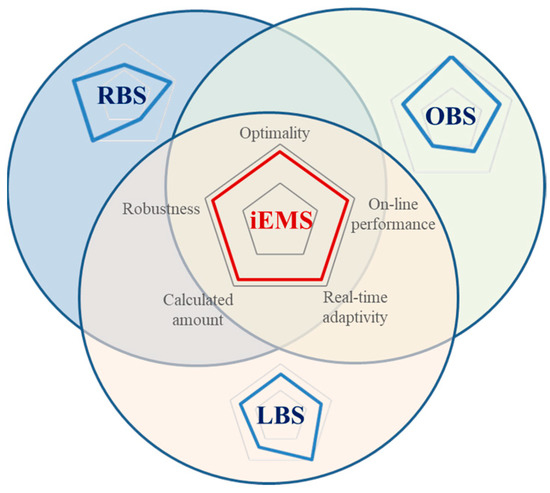
Figure 1.
The iEMS based on hybridization/nested concept.
Overall, the literature on the EMS is dense, and designing an EMS for a specific purpose can be tremendous work. The primary purposes of this work are (i) to propose an innovative EMS aiming for the real-time integration (strong constraint) of the FCS in the electric vehicle and (ii) to demonstrate the effectiveness and utility of the integrated EMS (iEMS) framework (introduced in [12]) in the process of developing such a complex control system. The iEMS is designed to tackle real-time challenges with a hybridization/nested concept approach that leverages the strengths and compensates for the weaknesses of each strategy. As illustrated in Figure 1, the iEMS solution is based on a simple concept that combines an optimal online OBS to optimize fuel consumption, an RBS to manage the electrical energy/power assist, and an LBS to successfully adapt the iEMS to the vehicle’s real-time environment.
The main objectives of this work are to:
- Provide a systematic and methodological approach to the design of complex EMSs (i.e., the iEMS framework: a new paradigm);
- Improve fuel consumption using the optimization concept;
- Be adapted to real-time driving conditions (stochastic behavior, possibility of integrating other constraints from the cooperative environment);
- To integrate the challenging fuel cell system into the electric vehicle (slow dynamic, downsizing, etc.).
The remainder of this paper is organized as follows: Section 2 deals with the related works. Section 3 addresses the design of our real-time iEMS. Section 4 presents the results and contrasts them with real-time data. Finally, some concluding remarks are made in Section 5.
In the following Section, we will further analyze the problem of the real-time iEMS applied to the FCHEV and identify the relevant research challenges. Then, our new approach based on the iEMS system is detailed according to our use case: FC/battery hybrid system. The OBS, RBS, and LBS development and combination are explained. Finally, the iEMS is validated through a 27-h real-time database and shows promising results [13].
2. Related Works
One of the main goals of the EMS is to reduce fuel consumption according to the driving requirements and the components’ constraints. Regardless of the technique, the EMS problem consists of the instantaneous management of the requested power throughout the hybrid energy storage system (HESS). While the command is local in time, the objectives are integral (e.g., fuel consumption) and semi-local (e.g., drivability). The state and control variable constraints are local in time (e.g., power threshold) and global. These characteristics make the optimal control problem more complex in real-time operating conditions. In this context, we proposed the iEMS concept combining the three families of the EMS. The first family consists of the OBS designed to find the optimal control behavior but has two main drawbacks: its online adaptation and real-time driving conditions adaptivity. The second one is the RBS, which can overcome the first limitation by providing expert or fuzzy rules to adapt a classical offline OB-EMS into an online OBS. Whilst the last one is the LBS, that can counteract the second limitation by processing the stochastic data from the cooperative environment to support the OBSs second disadvantage (see Figure 2). Finally, the control strategy designed with the iEMS concept combines:
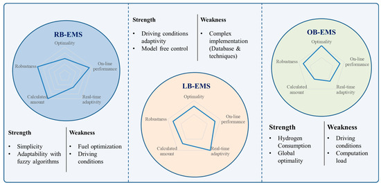
Figure 2.
Strengths and limits of the classical EMS categories.
- -
- OBS to meet the EMS central objective (i.e., consumption reduction);
- -
- RBS to adapt the OBS online;
- -
- LBS to adapt the RB-OBS to the environment stochastic behavior.
With this combined approach, choosing the appropriate technique for each level is crucial to provide relevant results without demanding an excessive development and computing capacity. The current choices enable us to obtain simple and realistic system behaviors with an acceptable computing time.
2.1. The Optimization-Based Strategy (OBS) Challenges
This EMS family is based on solving an optimization problem, for which dynamic programming (DP) is the most studied OBS. Prior knowledge of the driving cycle is required to discretize the problem and decompose it into sub-problems. It recursively computes the least cost path (i.e., the optimal sequence of commands), which can be computed from the global velocity information and optimal energy distribution of the two energy sources by minimizing a consumption function while considering the system constraints [14,15,16].
DPs main challenges are its “curse of dimensionality” [14], a very high computational cost, and the fact that the driving cycle information must be known in advance. Thus, DP is not adapted to real-time operating conditions.
However, several studies have been conducted to adapt DP to an online algorithm [15,17]. These methods adapt the DP algorithm to a local optimization algorithm. In [15], local linear and quadratic approximations of the cost-to-go function are proposed to reduce the DP computation load. In [14,18], driving prediction techniques (DPT) are used to estimate the driving cycle on a prediction horizon on which the DP algorithm is applied. In [19], the author proposed a stochastic DP (SDP) EMS based on a stochastic trip model prediction. DP has also been combined with RBS to propose an online solution using, for example, the power distribution schemes technique [20].
The online adaptation of the DP could be a promising strategy for iEMS, which is highly dependent on the prediction precision of the driving cycle. Automated connected vehicles and vehicle cloud data using vehicle-to-everything information are currently being deployed. Thanks to this newly available data, driving cycle prediction could be accurate enough to use optimization strategies (e.g., DP) on a prediction horizon. Nonetheless, the DPs curse of dimension remains, making them particularly inappropriate. Another similar optimization algorithm with a lower computational cost is the Pontryagin’s minimum principle (PMP). It represents an up-and-coming alternative for iEMS [21,22,23].
The PMP provides close optimal results as the DP through instantaneous optimization. Some comparative studies have shown a non-significant difference in energy saving, typically less than 2% [23]. Its instantaneous calculation of the optimal control makes it better adapted to online implementation, but it requires an appropriate optimal co-state computation, which is the core of the PMP process. While showing optimal performance under testing cycles used in the EMS design, it shows suboptimal results in real-time operating conditions.
Moreover, another OB-EMS was introduced in 1999 based on engineering intuition and since has been applied in many studies [24]. The equivalent consumption minimization strategy (ECMS) takes the electrical assistance as a buffer formulated as an equivalent fuel consumption unit that will eventually be charged thanks to the fuel or regenerative braking. The ECMS solves the optimization problem by instantaneously finding the minimum of the total equivalent power consumption. In some studies, the ECMS and PMP were proven to be equivalent, with differences in the optimization formulation [25].
2.2. Learning-Based Strategy (LBS) Integration
In addition, the ECMS has been validated and improved thanks to the PMP concept [25]. They rely on the instantaneous calculation of the equivalent factor (ECMS) or the co-state variable (PMP). However, their calculation is not straightforward according to the stochastic behavior of real-time operating conditions. Thus, A-ECMS and A-PMP have been proposed, integrating driving pattern recognition to support the strategy and proving that LBS can enhance the OB-EMS by adapting it to real-time operating conditions [26,27,28].
Driving patterns are classically classified into four classes: urban, suburban, main road, and highway driving patterns, and they are considered to remain the same over a selected segment [29]. Features must be selected to classify the driving pattern. The main features are segment energy and mean velocity [30]. In [31], the mean and maximum speed features are considered through a fuzzy classification. However, not enough real-time data were considered.
Furthermore, as the driving pattern recognizer LBS supports one specific EMS for one specific vehicle topology, the classification should be adaptively established according to the needs of the iEMS. The FCS integration requires a high controllability over the high absolute acceleration phases. However, the mean velocity has much more weight than the mean acceleration feature in the driving pattern identification [30]. In addition, acceleration is a feature characterizing the driver’s behavior [32].
Therefore, a new driving pattern recognition adapted to the FCHEV topology should be designed. The FCHEV-adapted driving pattern recognizer should be based on a central feature as the mean velocity to consider the typical classification while integrating acceleration. This way, the driving pattern information would combine typical driving patterns, driver’s behavior, and transitory phase information.
2.3. Rule-Based Strategy (RBS) and Engineering Intuition
Nonetheless, the PMP and ECMS real-time performances do not only rely on the driving pattern data. The equivalent factor and co-state optimality rely heavily on the vehicle state. Thus, in addition to the driving pattern, the SOC consideration must be integrated into the iEMS. The PMP optimality classically relies on the equality condition that the SOC targeted at the end of the input cycle being the same as the initial SOC. However, this can result in a charge-sustaining strategy for online applications because of the limited control over the SOC.
Therefore, engineering intuition suggests that maintaining the PMP offline global optimality is unnecessary for the online PMP. Instead, a solution must be developed to manage the using battery. Moreover, it has been shown that PMP optimality can be obtained even if the SOC targeted at the end of the cycle is different from the starting SOC [33]. Consequently, a new iEMS should adapt the PMP online application by managing the SOC targeted at each PMP sliding window final time to permit a suitable SOC liberty controllability under real-time operating conditions.
Therefore, according to the iEMS concept, our RBS should be developed to:
- -
- Combine the vehicle state expert knowledge with the hybrid control strategy;
- -
- Adapt the PMP algorithm according to the new battery usage engineering intuition.
2.4. Research Gap
We can find many state-of-the-art reviews in the literature, classifying and explaining the strength and limits of the three families of the EMS (i.e., OBS, RBS, LBS) [2,6,10,34]. Even some are specific to fuel cell vehicles [35]. Nonetheless, very few discuss combining the three EMS families and the iEMS concept [2], and none are developing how this promising framework would work.
However, choosing the proper EMS technique is a challenging task. Many different techniques are available, each with their strengths and weaknesses. For example, optimization-based strategies are effective at maximizing energy efficiency but can be computationally expensive and may not be suitable for real-time applications. Rule-based strategies are easier to implement and can provide an exemplary performance in certain conditions, but they may not be able to adapt to changing conditions. Learning-based strategies can adapt to changing conditions and optimize energy efficiency over time but may require significant amounts of data to train and may not be as reliable as other techniques.
Additionally, the choice of EMS technique may depend on factors such as the vehicle type, the energy storage system, and the driving conditions. The complexity of the decision-making process can be further compounded by the need to balance conflicting objectives, such as energy efficiency, energy sources’ health, and real-time performance.
In summary, the complexity of designing a real-time EMS with a specific aim and choosing the proper EMS technique are key pain points in developing energy management systems. However, research advances and the increasing availability of data are helping to address these challenges and enable the development of a more effective and efficient EMS.
2.5. The iEMS Concept: Combining the Three Families of Algorithms
Combining the three families of the EMS is beneficial for designing a real-time EMS as it allows for a more comprehensive and adaptive EMS. OBS, RBS, and LBS all have their strengths and weaknesses, and by combining them, the energy management system can take advantage of each strategy’s strengths while mitigating its weaknesses. This is particularly important for fuel cell vehicles, where the energy flow must be carefully managed to ensure the proper operation and performance of the vehicle.
In [12], we proposed such a framework designed to simplify EMS development. Furthermore, we oriented our approach to one of the most challenging automotive industry EMS: the fuel cell vehicle. The iEMS concept proposes a well-suited architecture to tackle the FCHEV real-time control strategy challenges. We have also proposed great candidate techniques to illustrate a possible combination. As such, the objectives of the work are to (i) propose an innovative EMS aiming for the real-time optimality of the fuel cell vehicle and (ii) to demonstrate the utility and functionality of the integrated EMS (iEMS) framework in the process of developing such a complex control system. In this way, researchers and engineers may have a new convenient tool to design a complex EMS or help them take a step back to further optimize their energy management systems.
2.6. Our iEMS Proposition
To demonstrate the utility of the iEMS concept in designing and tuning an EMS, we have chosen the promising techniques previously discussed previously.
As the OBS of the control architecture, the online PMP has shown appropriate qualifications to meet the primary goal of the EMS: reducing consumption. The literature indicates that driving patterns must support the PMP to adapt the iEMS to the stochastic behavior of the driving conditions. Furthermore, the classification of the driving patterns should be tailored to the vehicle topology and the driver’s behavior. Therefore, a suitable LBS for the iEMS architecture is a driving pattern recognizer based on an innovative driving conditions classification. Finally, the classical online PMP must be adapted to a new version where the SOC controllability is improved according to the engineering intuition of battery usage. So, the RBS of the iEMS should integrate the vehicle state expert knowledge and the driving pattern into a battery usage strategy in the service of the OBS.
Furthermore, the iEMS concept focuses on achieving optimal system control under real-time operating conditions. Hence, it is necessary to use real-time measured data rather than relying on normalized cycles.
3. Integrated Energy Management Strategy iEMS Development
3.1. System Modeling
The iEMS developed in this paper aims to tackle the FCS integration into the everyday vehicle. Considering the FCHEVs price and energy control complexity problems, we choose a battery as the electrical assistance to support the FCS energy and power capability. Then, we choose the two converters’ parallel architecture for maximum controllability [4], illustrated in Figure 3. The focus of this work is the HESS energy flow. The system modeling approach is relevant as the EMS commands the energy node.
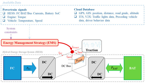
Figure 3.
The global architecture of the FCHEV topology.
This work has been conducted to easily be reproduced on most FCHEV sizes. Therefore, we designed our system using typical vehicle characteristics according to the result of the sizing methodology proposed in [36].
- Vehicle Modeling
The traction power to propel the vehicle can be expressed as:
where is the longitudinal vehicle velocity, is the vehicle mass, is the gravitational force, is the equivalent longitudinal aerodynamic drag force, and is the force due to the rolling resistance.
Then, the bus power , which is the power requested on the electric node by the motor, is calculated by:
where is the DC/AC motor converter yield, and is the motor yield.
The bus, battery, and FCS net power intersect on the electric node. The following equation governs it:
where is the FCS converter yield, is the FCS net power, is the battery converter yield, and is the battery power.
- Battery Modeling
Due to its practicality, the enhanced simple battery model is often used for energy management systems’ design [25,37]. It considers the SOC effect on the battery’s internal resistance. Then, the battery trajectory can be calculated as:
where is the time derivative of the battery state of charge (SOC), is the Coulombic efficiency, is the battery open circuit voltage, is the battery’s internal resistance, is the battery capacity, and is the battery output power.
- Fuel Cell System Modeling
The FCS size is designed using the multi-criteria and optimal approach introduced in [36]. The hydrogen consumption rate of a fuel cell can be calculated by:
where is the number of cells, is the hydrogen molar mass, is the transferred electrons, is Faraday’s constant, and is the FCS stack current.
The FCS net or output power is given by:
where is the FCS consumed power, and is the FCS auxiliaries power.
Then, the FCS efficiency is calculated by:
where is the FCS efficiency, and is the hydrogen lower heating value.
To evaluate the cost of hydrogen consumption, we designed a second-order polynomial interpolation of the FCS fuel power , illustrated in Figure 4. As we will see through the Hamiltonian function formulation in Section 3.3.2, this finding was made to support the PMP online application in expressing the cost function (i.e., ) according to the command variable (i.e., ).
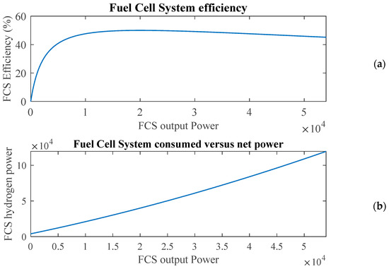
Figure 4.
(a) Fuel cell system used efficiency; (b) fuel cell system used versus output power.
The FCHEV model was designed to be easily adapted to the broadest range of sizing applications and to propose an intelligent tradeoff between the precision and practicality for the online iEMS.
3.2. iEMS Global Architecture
Three imbricated categories of energy management strategies were developed and combined to answer the complex problem of the real-time EMS discussed in Section 2. The global architecture of the iEMS is presented in Figure 5 and highlights the OBS, LBS, and RBS synergy, with the PMP overseeing the fuel consumption reduction objective. In this Section, we will present each strategy from right to left.

Figure 5.
Proposed iEMS global architecture.
3.3. The OBS: Online PMP
The main objective of the iEMS system is to reduce fuel consumption. As discussed in Section 2, the online PMP is well-suited for this task. The PMP proposes a solution to the optimization problem.
3.3.1. Optimization Problem Formulation
- State equation
Let us consider a system described with the state equation:
where is the state vector, and is the control variable. We formulate the optimization problem using the power-based formulation suitable for the EMS [25]. Therefore, the state variable is the electrochemical energy variation given by:
where is the total capacity of the battery, and is the initial time. Then, the control variable is the FCS net power . Then, using Equations (3) and (9) in Equation (4), the state Equation (8) can be formulated as:
- Local state and control variable constraints
Limited by the HESS technology and sizing, the state and control variable must stay within a range of admissible boundaries. Moreover, we choose to add a rate limitation to the control variable as it is crucial for FCS health. Hence, the state and control variables’ local constraints can be described with the following set of inequalities:
where is the upper SOC boundary, is the lower SOC boundary, is the maximum FCS output power, is the minimum FCS output power, is the one-time time derivative of the control variable, and is the constant variation limit enforced to the FCS net power.
- Boundary conditions
The final state variable condition must be known a priori for the PMP algorithm to converge. As seen in Section 2, the classical and offline optimal solution is to enforce , where is the final time of the PMP input cycle and is the starting time. However, we have covered in the first Section that the online application of this hard constraint implies a charge-sustaining strategy, which is far less optimal than the offline PMP. Therefore, in this paper, one considers the targeted SOC as a dynamic input of the PMP algorithm. Hence, the boundary conditions on any prediction horizon, that is, on any interval ], are:
where is the data prediction horizon, and is the targeted by the online PMP algorithm. The strategy for its calculation is proposed in the next Section.
- Performance index and cost function
Finally, the cost function can be introduced. The optimal control problem is to find the optimal control sequence that minimizes the performance index :
where is the penalty function. In this paper, we did not consider a penalty function. Its tuning requires proper study, which should be considered after completing the iEMS design.
- Optimization problem formulation
The constrained-finite time horizon optimal control problem consists of finding the control sequence that minimizes the performance index while meeting the state and control variables’ local constraints and the dynamic constraints given by Equation (11). More details can be found by consulting [25] to extend further the optimal control theory and its application.
The following Section proposes a solution to the online optimization problem applied to the FCHEV using Pontryagin’s minimum principle (PMP).
3.3.2. Online Pontryagin’s Minimum Principle
- Hamiltonian function
The Pontryagin’s Minimum Principle provides a necessary condition to solve the optimization problem:
where is the Hamiltonian function, is the optimal command, and is the co-state variable.
In our case, we use the power-based formulation of the Hamiltonian function, which is given by:
The right-hand side of the Hamiltonian function is the system trajectory; that is, the state Equation (10) multiplied by the costate variable . The latter is the tuning parameter of the PMP. When the absolute value of the co-state increases, the overall battery usage (i.e., the input cycle final SOC) decreases.
The left-hand side of the Hamiltonian is the cost function expressed according to the control variable through the polynomial approximation of the efficiency, as seen in Figure 4. Our polynomial function can be easily adapted to other FCS sizing and performance by tuning its coefficient and is given by:
For our use case, the coefficient of the cost function was tuned as a = ; b = 1.6; c = 4000.
- PMP online algorithm
The proposed online PMP algorithm is based on the same principle as the offline PMP but with some key differences. As the offline PMP, our online algorithm considers a targeted SOC at the end of an input cycle (e.g., bus power request cycle) to converge; that is, to output the optimal sequence of command (i.e., the FCS net power command). The difference is that the targeted SOC is not obtained through equality with the initial SOC. Instead, our new online PMP algorithm considers the targeted SOC as a dynamic input that will be used as the final condition of the current PMP iteration. Hence, our PMP algorithm is executed on each -second sliding window, where is the prediction horizon. The considered PMP algorithm operation on any sliding window is detailed in Algorithm 1. Moreover, we fixed the prediction horizon to 7 s based on the study presented in [17], which showed that this value is the shortest horizon to enable global optimality using the dynamic programming algorithm.
In order to ensure that our online PMP algorithm can converge on a given sliding window , the following condition must be satisfied:
where is the desired precision in seconds that we tuned to .
The OBS online operation requires the targeted SOC at the end of each predicted cycle. Furthermore, the classical SOC target strategy (i.e., ) is not working for the online OBS. Considering this hard equality condition, the battery trajectory is constrained, and the EMS results are far from the desired (i.e., the optimality of the offline PMP). Therefore, the SOC target controllability is of the utmost importance. The innovation of the OBS algorithm considers a dynamic SOC target according to the strategy described in the next Section.
| Algorithm 1. The proposed online PMP algorithm operation on a sliding window |
If above and go to Step 2. If yes: output the optimal command vector. |
3.4. The RBS: Expert Rules and Fuzzy Inference System
As seen in Section 1, the literature indicates that the driving pattern and the SOC are the two parameters improving the online PMP performance. The driving pattern consideration enables the iEMS to adapt to the environment and the driver’s behavior. The SOC consideration adapts the strategy to the system’s internal state. Furthermore, the targeted SOC at the end of each prediction horizon must be cleverly managed for online PMP optimality. Therefore, we designed a “Battery Usage Strategy” based on expert rules and a fuzzy inference system in charge of calculating the SOC target according to the SOC and the driving pattern.
3.4.1. Expert Rules
The first step to designing the battery usage strategy is to manage the SOC target boundaries. If the targeted SOC obtained is outside the reachable SOC, the OBS will not converge, and the results will be sub-optimal. Nonetheless, as the SOC target boundaries must be calculated at the start of each PMP iteration (i.e., of each sliding window), we must monitor the extremum SOC variations from Hp seconds in advance, which is not trivial. The intuition would make us use the system trajectory given by Equation (10) and consider the maximum battery power for Hp seconds to calculate the upper boundary (respectively, the minimum battery power for the lower boundary). In addition, the control variable of the system is the FCS net power, which is linked to the battery power and the bus power by Equation (3). Therefore, not considering the FCS net power and the bus power occurring between the SOC target computation (i.e., at ) and the end PMP convergence, (i.e., at ) would result in unreachable boundaries. Since an unreachable final SOC is precisely what we must prevent, a solution based on the expert knowledge of the system is proposed. The solution aims to answer the question at the start of each PMP iteration: what is the set of a final admissible SOC (i.e., the SOC at the end of the PMP iteration)?
Then, the PMP-targeted SOC must be calculated considering the bus power prediction, which will be covered in future work, the battery power, and the FCS net power. The boundaries calculation of the final SOC is to determine the following:
- (i)
- The control variable boundaries on each time step of each sliding window;
- (ii)
- The battery power boundaries on each time step using (i) in Equation (3);
- (iii)
- The maximum variation in the SOC according to the real-time battery power boundaries using (ii) results in Equation (4) and by applying, if necessary, the constraints Equation (11).
The expert rules are described below by two sets of necessary conditions.
- Control variable boundaries:
- Local constraints on the battery power: prohibit wasting energy or having to supply too much power:where and are, respectively, the dynamic lower and upper battery power boundaries, and and are the lower and upper battery power global boundaries.
Finally, the target SOC boundaries on each sliding window are obtained using Equation (4):
where and are the lower and upper targeted SOC boundaries, respectively, and is the PMP algorithm sample time that we fixed to 1 s to master the online computation burden.
Thanks to this set of expert rules that define the admissible set of the targeted SOC, the SOC target will be reachable by the battery, and therefore the PMP will converge. The next step is to develop a system that chooses a candidate between the admissible SOC target.
3.4.2. Fuzzy Inference System
The second step of the battery usage strategy (i.e., the RBS) consists of designing an intelligent system using the SOC and the driving pattern to monitor the battery usage. A fuzzy inference system with the SOC and the driving pattern as the input and the battery usage percentage as the output is designed.
- Inputs Fuzzification
While the SOC range is [0;100], the driving pattern range is [1;5]. We based the considered driving patterns on our classification presented in the next Section. They are: Traffic, Urban, Main Road, Highway, and Sportive driving modes; see Figure 6.
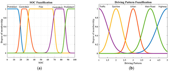
Figure 6.
(a) “Battery SOC fuzzification”; (b) “Driving Patterns Fuzzification”.
- Fuzzy Logic Controller Strategy
The strategy adopted is presented through a fuzzy logic controller (FLC) control surface, as shown in Figure 7. For example, we see that on the Prohibited SOC range (i.e., ), our FLC will calculate 0 to 0.1% of battery usage. Concerning the driving patterns, we see that the FLC will compute a lower battery usage for the Highway driving pattern than for the Urban driving pattern. Furthermore, the designed controller will compute the highest battery usage for the Sportive driving pattern.
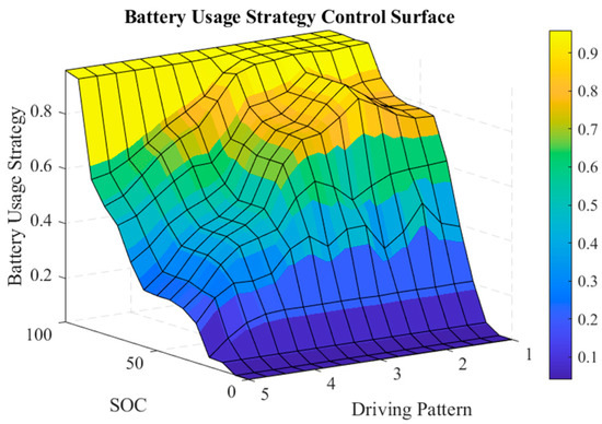
Figure 7.
Control surface of our battery usage strategy.
Thanks to the online fuzzy logic controller, the battery usage is defined at the start of each sliding window.
Finally, thanks to the SOC target boundaries given by Equation (20), the SOC target is obtained by:
where is the targeted SOC, is the percentage of battery usage given by our fuzzy logic, and and are the SOC target boundaries calculated thanks to our RBS expert rules covered in the previous subsection.
The RBS efficiency relies on the driving pattern efficiency, which implies that high absolute acceleration phases will result in the poor performance of the FCHEV system if not controlled accurately. The iEMS RBS layer considers the driving pattern to control the battery usage strategy accordingly. Therefore, the iEMS performance relies on the driving pattern, which must be adapted to the FCHEV topology to maintain a good controllability during acceleration phases and improve the overall performance of the iEMS.
3.5. The LBS: Driving Pattern Recognizer Designed for FCHEVs
The driving pattern recognizer must include an intelligent well-suited characterization of the driving pattern. As discussed in Section 2, the inputs of our system (i.e., chosen feature parameters) are velocity and acceleration. We have developed the driving pattern recognizer in four steps: (i) database preprocessing, (ii) data standardization, (iii) clustering, and (iv) online DPR modeling.
3.5.1. Fuzzy C-Means Classification of the Driving Patterns
- Database processing
The classification database must represent the real-time driving conditions: we choose a database containing 27-h of real-time trip data [13]. The classification database was then constructed with the extracted time, velocity, and acceleration. Figure 8 illustrates the database preprocessed through two interesting intervals selected from the database validation partition, which we choose to test our iEMS in the next Section. The classification database must reflect the complexity and variability of actual driving conditions to accurately classify the driving patterns.
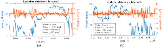
Figure 8.
Two interesting intervals extracted from the 27-h real-time measured database (a) Interval1; (b) Interval2.
- Data standardization
The data standardization must be conducted carefully, considering the real-time data collection and the FCHEV system’s requirement. However, we found that the negative acceleration compensates for the positive acceleration. Thus, the first step of the data processing is to take the absolute value of the accelerations.
Then, real-time data collection is conducted by averaging the velocity and acceleration on a past horizon. We tune this parameter to 7 s. Then, the second step of the data processing is to average the real-time database per past the horizon segment.
The FCHEV system’s performance is sensitive to the high absolute acceleration phases. Therefore, the clustering process must not favor the velocity over the acceleration. However, the range of acceleration is more than fifteen times lower than the velocity range. Thus, the second step of the data processing is to normalize between the acceleration and the velocity. The goal here is to prohibit the learning process from favoring the velocity, of which the range of is much higher than the acceleration. Thanks to this step, a high acceleration cluster has shown up. That enables the RBS to demonstrate a higher controllability of our highly acceleration-dependent system.
- Classification
We used a clustering approach to classify the driving patterns in our data, which involves grouping the data points into clusters based on their similarity. To determine the optimal number of clusters, we used the Calinski–Harabasz clustering evaluation criterion. Five distinct clusters were found, which correspond to five driving patterns. They can be called: Traffic (low velocity), Urban, Main Road, Highway, and Sportive (high acceleration); see Figure 9. The sportive driving pattern appearance shows that our data classification successfully answers our double objective: the FCHEV topology sensibility and driver’s behavior characterization.
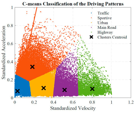
Figure 9.
Classification of the driving patterns.
3.5.2. Online Driving Pattern Recognizer
From this classification designed for FCHEVs, we developed the online DPR using the fuzzy C-means clustering technique. The DPR control surface was generated from the labeled database and will allow us to continuously classify the driving patterns in real-time (Figure 10).
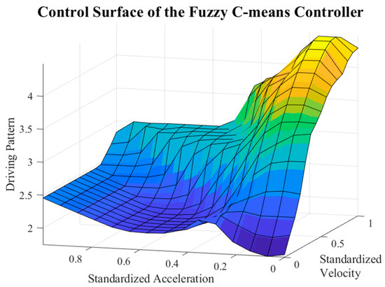
Figure 10.
The control surface of the driving pattern recognizer.
4. Results and Discussion
Our iEMS operation is described in Figure 5. We used the data from the real-time database presented in the previous Section to validate our results for each strategy, which will be presented from left to right. Two of the most significant intervals are used to illustrate the results; see Figure 8. Lastly, our online iEMS is compared to the optimal offline PMP algorithm result.
4.1. The Driving Pattern Recognizer LBS
The DPR takes the standardized velocity and acceleration as the input and provides the driving pattern as the output; see Section 3.5. The LBS results are shown in Figure 11, using the first interval.
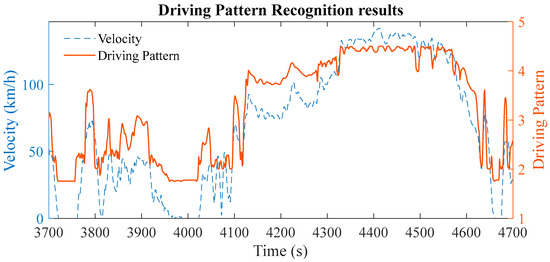
Figure 11.
Our new driving pattern recognizer results on Interval1.
From 3700 s to 4100 s, where the velocity varies from 0 to 50 km/h, we notice that the driving patterns recognized are between Traffic and Urban, except between 3780 s and 3800 s, where the velocity increases to 80 km/h. Here, the Main Road driving pattern is recognized.
Then, from the time interval [4350 s; 4550 s], the velocity is over 120 km/h, and the driving patterns recognized are between the Main Road and Highway.
Furthermore, we can note that our new high-acceleration-dependent DPR successfully recognized the high-acceleration phases by accurately recognizing the sportive driving pattern during the fast variation in the velocity. Our innovative LBS successfully characterizes the different phases needed to provide high controllability to the iEMS.
4.2. Battery Usage RBS
The battery usage strategy outputs are the battery usage percentage according to the LBS output (i.e., the driving pattern) and the SOC. The RBS results are shown in Figure 12.
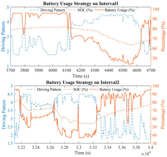
Figure 12.
Battery usage strategy results.
From 3850 s to 4550 s and from 33,300 s to 34,000 s, where the driving pattern is between Sportive and Urban, and the SOC is in its free range (see Figure 6), the outputted battery usage is the highest (between 80% and 100%). This should be the case since the SOC and acceleration demand are high.
Then, from 4350 s to 4550 s where the driving pattern is between Main Road and Highway, the Battery Usage decreases to 40%. Between 32,800 s and 33,200 s, where the driving pattern is in the same range, but the SOC is lower, the outputted Battery Usage is even lower, reaching almost 30%.
Furthermore, the rising spikes, occurring when the SOC is in its Controlled range (i.e., around 20 to 40%), show that the battery usage strategy can provide enough power in a short time if needed.
Thanks to our drivers’ behavior and FCS-adapted DPR, and then to the FLC battery usage strategy, the fast-changing driving patterns are covered by the battery usage and will provide a precise direction to the decision algorithm; that is, the OBS.
4.3. The iEMS Results
Thanks to the LBS and the RBS, the battery usage percentage was obtained. Then, Equation (21) made the SOC target available for the PMP. Figure 13 shows the optimality of our online PMP algorithm. The computation of the costate is compared with the offline PMP costate.
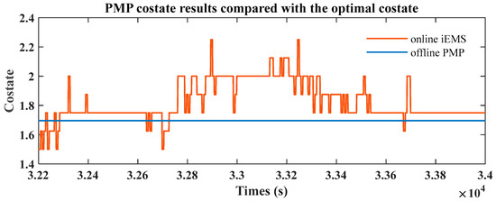
Figure 13.
Online PMP costate results compared with the optimal PMP on the selected window.
The results show that the online computed costate oscillates around the offline PMP, thus validating the fuel consumption optimization process.
Finally, the three families of the EMS are combined through our iEMS. Its outputs are the battery and FCS net power command. Figure 14 shows the iEMS results. The SOC is the lowest at time 33,060 s (Figure 14b), which is how we selected the first interval (Figure 14a). Figure 14b shows the SOC variation during the 27-h real-time trips and compares the iEMS results with the offline PMP.
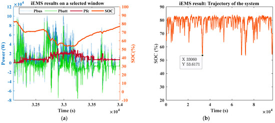
Figure 14.
(a) iEMS results on a selected window; (b) iEMS compared with the optimal offline PMP.
The results show that the battery answers the high bus power requests according to the FCS integration constraints. The FCS provides energy in a relatively steady manner and does not idle, respecting the fuel cell technology health specifications. Furthermore, the iEMS results show that the fuel consumption is under 1.1%, which is as optimal as the online and offline PMP (see Figure 14b). These results are possible and consistent thanks to the iEMS concept allowing the PMP convergence condition (i.e., the sliding windows SOC target) to be computed in real-time by combining our FCHEV-adapted DPR and its corresponding battery usage strategy FLC and expert rules.
4.4. Discussion
To compute the amount of dihydrogen ( consumed by a proton exchange membrane fuel cell (PEMFC) to produce 118.94 kWh of electrical energy at the output of the PEMFC, we can use the lower heating value (LHV) of hydrogen and the efficiency of the PEMFC.
Assuming a PEMFC efficiency of 50% (may be adapted according to the technology), we can calculate the mass of hydrogen consumed as follows:
where is the mass of consumed in kilograms, is the energy produced by the FCS at the electric node (cf. Figure 3) in kWh, and is the PEMFC efficiency.
Assuming an LHV of 120.1 MJ/kg for hydrogen and a 0.95 convertor efficiency, we obtain a consumed mass of 7.506 kg.
Furthermore, the total distance corresponding to the entire database is 1281 km. Then, the consumption assessment is around 0.58 kg/100 km.
Therefore, our iEMS, with an assumed efficiency of 50%, would consume approximately 0.58 kg/100 km of dihydrogen in real-time operating conditions.
To contrast this result, we have to (i) compare it with actual fuel cell vehicle consumption, and (ii) discuss the potential biases.
In [38], the Toyota Mirai dihydrogen consumption was measured from 0.98 to 1.05 kg/100 km on standardized cycles. In [39], the Hyundai Nexo reportedly had a 0.67 kg/100 km consumption in urban-type driving. That means our potential improvement range would be between 13% and 45%.
Our proposed iEMS, designed using an extensive real-time driving conditions database, show promising results, allowing for a considerable dihydrogen consumption margin for adapting it to real-time testing. The iEMS concept is proven to significantly help design complex energy management systems such as the challenging FCHEVs’ EMSs.
5. Conclusions
A methodological solution to the FCS integration into the electric vehicle and its fuel consumption optimization under real-time trip operating conditions was proposed in this paper. We demonstrated the utility of our proposed iEMS framework in simplifying and improving the energy control of complex systems. It was based on an imbricated concept, combining the three classical categories of the EMS to achieve several objectives.
To tackle the overall objective of the real-time optimization of energy consumption considering the FCS integration challenges, we developed an original approach based on a real-time adaptation of the offline PMP. The proposed optimal online PMP combines a new FCHEV-adapted driving pattern recognizer and a fuzzy battery usage strategy to compute the targeted SOC on each sliding window.
Following the iEMS concept, each strategy adds advantages to compensate for the other limits. We adapted the offline optimal PMP to an innovative online PMP by integrating a dynamic SOC target input to optimize fuel consumption. To accurately compute the SOC target, we designed a battery usage strategy based on fuzzy and expert rules considering driving patterns and the SOC as the inputs.
Finally, we developed a new driving pattern recognition algorithm specifically adapted to the FCHEV topology. It added adaptability and controllability to iEMS. The proposed algorithm is validated on a database of 27-h of real-time trips.
This paper demonstrates the innovative iEMS architecture through a set of chosen and FCHEV custom-made techniques.
This work is part of the hydrogen deployment supported by governments and the European Union (e.g., France 2030, Horizon Europe). This work opens perspectives for our laboratory to position itself on international collaborations in the framework of European project funding.
Future works should be conducted mainly on three prospects. First, the velocity prediction on the 7 s sliding windows was considered ideal, but it is a sub-system of our iEMS. The fuel consumption optimality of the iEMS depends on this sub-system. Therefore, adapting it to real-time driving conditions is crucial to achieving the best performance. We will present our proposed solution to address this challenge in a future work.
Second, we will conduct experiments in a realistic traffic and virtual reality environment to test the iEMS in real-time conditions beyond the 27-h real-time trip database.
Finally, we will experimentally validate our proposed approach on a fuel cell hybrid electric vehicle prototype.
Author Contributions
Conceptualization, M.M. (Matthieu Matignon); methodology, M.M. (Matthieu Matignon); software, M.M. (Matthieu Matignon) and A.C. (Adriano Ceschia); validation, M.M. (Matthieu Matignon), T.A. and M.M. (Mehdi Mcharek); formal analysis, M.M. (Matthieu Matignon); investigation, M.M. (Matthieu Matignon); resources, M.M. (Matthieu Matignon); data curation, M.M. (Matthieu Matignon); writing—original draft preparation, M.M. (Matthieu Matignon), T.A. and M.M. (Mehdi Mcharek); writing—review and editing, M.M. (Matthieu Matignon), T.A., M.M. (Mehdi Mcharek), and A.C. (Ahmed Chaibet); supervision, T.A., M.M. (Mehdi Mcharek), and A.C. (Ahmed Chaibet); project administration, T.A., M.M. (Mehdi Mcharek), and A.C. (Ahmed Chaibet). All authors have read and agreed to the published version of the manuscript.
Funding
This research received no external funding.
Data Availability Statement
The database used for this work is open source. Here is a link for the 70 driving cycles database: https://ieee-dataport.org/open-access/battery-and-heating-data-real-driving-cycles (accessed on February 2023).
Conflicts of Interest
The authors declare no conflict of interest.
Abbreviations
| Acronym | Meaning |
| EMS | Energy management strategy |
| OBS | Optimization-based strategy |
| RBS | Rule-based strategy |
| LBS | Learning-based strategy |
| SOC | (Battery) state of charge |
| FCS | Fuel cell system |
| FCHEV | Fuel cell hybrid electric vehicle |
| HESS | Hybrid energy storage system |
| DP | Dynamic programming |
| PMP | Pontryaguin minimum principle |
| ECMS | Equivalent consumption minimization strategy |
| LHV | Lower heating value |
References
- Sorlei, I.-S.; Bizon, N.; Thounthong, P.; Varlam, M.; Carcadea, E.; Culcer, M.; Iliescu, M.; Raceanu, M. Fuel cell electric vehicles—A brief review of current topologies and energy management strategies. Energies 2021, 14, 252. [Google Scholar] [CrossRef]
- Tran, D.-D.; Vafaeipour, M.; El Baghdadi, M.; Barrero, R.; Van Mierlo, J.; Hegazy, O. Thorough state-of-the-art analysis of electric and hybrid vehicle powertrains: Topologies and integrated energy management strategies. Renew. Sustain. Energy Rev. 2020, 119, 109596. [Google Scholar] [CrossRef]
- Luo, Y.; Wu, Y.; Li, B.; Qu, J.; Feng, S.-P.; Chu, P.K. Optimization and cutting-edge design of fuel-cell hybrid electric vehicles. Int. J. Energy Res. 2021, 45, 18392–18423. [Google Scholar] [CrossRef]
- Azib, T.; Larouci, C.; Chaibet, A.; Boukhnifer, M. Online energy management strategy of a hybrid fuel cell/battery/ultracapacitor vehicular power system. IEEJ Trans. Electr. Electron. Eng. 2014, 9, 548–554. [Google Scholar] [CrossRef]
- Ritzberger, D.; Hametner, C.; Jakubek, S. A real-time dynamic fuel cell system simulation for model-based diagnostics and control: Validation on real driving data. Energies 2020, 13, 3148. [Google Scholar] [CrossRef]
- Zhang, F.; Wang, L.; Coskun, S.; Pang, H.; Cui, Y.; Xi, J. Energy management strategies for hybrid electric vehicles: Review, classification, comparison, and outlook. Energies 2020, 13, 3352. [Google Scholar] [CrossRef]
- Zhang, F.; Hu, X.; Langari, R.; Cao, D. Energy management strategies of connected HEVs and PHEVs: Recent progress and outlook. Prog. Energy Combust. Sci. 2019, 73, 235–256. [Google Scholar] [CrossRef]
- Jalil, N.; Kheir, N.A.; Salman, M. A rule-based energy management strategy for a series hybrid vehicle. In Proceedings of the 1997 American Control Conference (Cat. No. 97CH36041), Albuquerque, NM, USA, 4–6 June 1997; pp. 689–693. [Google Scholar]
- Erdinc, O.; Vural, B.; Uzunoglu, M. A wavelet-fuzzy logic based energy management strategy for a fuel cell/battery/ultra-capacitor hybrid vehicular power system. J. Power Sources 2009, 194, 369–380. [Google Scholar] [CrossRef]
- Salmasi, F.R. Control strategies for hybrid electric vehicles: Evolution, classification, comparison, and future trends. IEEE Trans. Veh. Technol. 2007, 56, 2393–2404. [Google Scholar] [CrossRef]
- Majed, C.; Karaki, S.H.; Jabr, R. Neural Network Technique for Hybrid Electric Vehicle Optimization. In Proceedings of the 2016 18th Mediterranean Electrotechnical Conference (MELECON), Lemesos, Cyprus, 18–20 April 2016. [Google Scholar]
- Matthieu, M.; Toufik, A.; Mehdi, M.; Chaibet, A. Real-time and multi-layered energy management strategies for fuel cell electric vehicle overview. In Proceedings of the 2022 IEEE 95th Vehicular Technology Conference:(VTC2022-Spring), Helsinki, Finland, 19–22 June 2022; pp. 1–6. [Google Scholar]
- Steinstraeter, M.; Buberger, J.; Trifonov, D. Battery and Heating Data in Real Driving Cycles. IEEE Dataport 2020. [Google Scholar] [CrossRef]
- Liu, J.; Chen, Y.; Li, W.; Shang, F.; Zhan, J. Hybrid-Trip-Model-Based Energy Management of a PHEV With Computation-Optimized Dynamic Programming. IEEE Trans. Veh. Technol. 2017, 67, 338–353. [Google Scholar] [CrossRef]
- Larsson, V.; Johannesson, L.; Egardt, B. Analytic Solutions to the Dynamic Programming Subproblem in Hybrid Vehicle Energy Management. IEEE Trans. Veh. Technol. 2014, 64, 1458–1467. [Google Scholar] [CrossRef]
- Gong, Q.; Li, Y.; Peng, Z.-R. Trip-Based Optimal Power Management of Plug-in Hybrid Electric Vehicles. IEEE Trans. Veh. Technol. 2008, 57, 3393–3401. [Google Scholar] [CrossRef]
- Yazdani, A.; Bidarvatan, M. Real-Time Optimal Control of Power Management in a Fuel Cell Hybrid Electric Vehicle: A Comparative Analysis. SAE Int. J. Altern. Powertrains 2018, 7, 43–54. [Google Scholar] [CrossRef]
- Liu, J.; Chen, Y.; Zhan, J.; Shang, F. An On-Line Energy Management Strategy Based on Trip Condition Prediction for Commuter Plug-In Hybrid Electric Vehicles. IEEE Trans. Veh. Technol. 2018, 67, 3767–3781. [Google Scholar] [CrossRef]
- Le Rhun, A. Stochastic Optimal Control for the Energy Management of Hybrid Electric Vehicles under Traffic Constraints. Ph.D. Thesis, Université Paris Saclay, Gif-sur-Yvette, France, 2019. [Google Scholar]
- Du, C.; Huang, S.; Jiang, Y.; Wu, D.; Li, Y. Optimization of Energy Management Strategy for Fuel Cell Hybrid Electric Vehicles Based on Dynamic Programming. Energies 2022, 15, 4325. [Google Scholar] [CrossRef]
- Boltyanskiy, V.G.; Gamkrelidze, R.V.; Pontryagin, L.S. Theory of Optimal Processes; Joint Publications Research Service: Arlington, VA, USA, 1961. [Google Scholar]
- Geering, H.P. Optimal Control with Engineering Applications; Springer: Berlin/Heidelberg, Germany, 2007. [Google Scholar]
- Kim, N.; Cha, S.; Peng, H. Optimal Control of Hybrid Electric Vehicles Based on Pontryagin’s Minimum Principle. IEEE Trans. Control. Syst. Technol. 2010, 19, 1279–1287. [Google Scholar]
- Paganelli, G. Conception et Commande d’une Chaîne de Traction pour Véhicule Hybride Parallèle Thermique et Électrique. Ph.D. Thesis, Université de Valenciennes, Valenciennes, France, 1999. [Google Scholar]
- Onori, S.; Serrao, L.; Rizzoni, G. Hybrid Electric Vehicles: Energy Management Strategies; Springer: Berlin/Heidelberg, Germany, 2016. [Google Scholar]
- Xie, S.; Hu, X.; Qi, S.; Lang, K. An artificial neural network-enhanced energy management strategy for plug-in hybrid electric vehicles. Energy 2018, 163, 837–848. [Google Scholar] [CrossRef]
- Li, H.; Zhou, Y.; Xiong, H.; Fu, B.; Huang, Z. Real-Time Control Strategy for CVT-Based Hybrid Electric Vehicles Considering Drivability Constraints. Appl. Sci. 2019, 9, 2074. [Google Scholar] [CrossRef]
- Li, H.; Ravey, A.; N’Diaye, A.; Djerdir, A. Online adaptive equivalent consumption minimization strategy for fuel cell hybrid electric vehicle considering power sources degradation. Energy Convers. Manag. 2019, 192, 133–149. [Google Scholar] [CrossRef]
- Zhou, Y.; Ravey, A.; Péra, M.-C. A survey on driving prediction techniques for predictive energy management of plug-in hybrid electric vehicles. J. Power Sources 2018, 412, 480–495. [Google Scholar] [CrossRef]
- Montazeri, M.; Fotouhi, A.; Naderpour, A. Driving segment simulation for determination of the most effective driving features for HEV intelligent control. Veh. Syst. Dyn. 2012, 50, 229–246. [Google Scholar] [CrossRef]
- Zhang, S.; Xiong, R. Adaptive energy management of a plug-in hybrid electric vehicle based on driving pattern recognition and dynamic programming. Appl. Energy 2015, 155, 68–78. [Google Scholar] [CrossRef]
- Lin, C.-C.; Jeon, S.; Peng, H.; Lee, J.M. Driving Pattern Recognition for Control of Hybrid Electric Trucks. Veh. Syst. Dyn. 2004, 42, 41–58. [Google Scholar] [CrossRef]
- Kim, N.; Rousseau, A. Sufficient conditions of optimal control based on Pontryagin’s minimum principle for use in hybrid electric vehicles. Proc. Inst. Mech. Eng. Part D J. Automob. Eng. 2012, 226, 1160–1170. [Google Scholar] [CrossRef]
- Saiteja, P.; Ashok, B. Critical review on structural architecture, energy control strategies and development process towards optimal energy management in hybrid vehicles. Renew. Sustain. Energy Rev. 2022, 157, 112038. [Google Scholar] [CrossRef]
- Zhao, X.; Wang, L.; Zhou, Y.; Pan, B.; Wang, R.; Wang, L.; Yan, X. Energy management strategies for fuel cell hybrid electric vehicles: Classification, comparison, and outlook. Energy Convers. Manag. 2022, 270, 116179. [Google Scholar] [CrossRef]
- Ceschia, A.; Azib, T.; Bethoux, O.; Alves, F. Multi-Criteria Optimal Design for FUEL Cell Hybrid Power Sources. Energies 2022, 15, 3364. [Google Scholar] [CrossRef]
- Saldaña, G.; Martín, J.I.S.; Zamora, I.; Asensio, F.J.; Oñederra, O. Analysis of the Current Electric Battery Models for Electric Vehicle Simulation. Energies 2019, 12, 2750. [Google Scholar] [CrossRef]
- Wang, T.; Jia, G.; He, S.; Lei, N.; Kang, Z.; Zou, D.; Zhang, Q.; Kou, W.; Xia, L. Experimental Study on The Performance of FCV in Standard Test Cycle. IOP Conf. Ser. Earth Environ. Sci. 2021, 632, 032014. [Google Scholar] [CrossRef]
- Sery, J.; Leduc, P. Fuel cell behavior and energy balance on board a Hyundai Nexo. Int. J. Engine Res. 2021, 23, 709–720. [Google Scholar] [CrossRef]


Disclaimer/Publisher’s Note: The statements, opinions and data contained in all publications are solely those of the individual author(s) and contributor(s) and not of MDPI and/or the editor(s). MDPI and/or the editor(s) disclaim responsibility for any injury to people or property resulting from any ideas, methods, instructions or products referred to in the content. |
© 2023 by the authors. Licensee MDPI, Basel, Switzerland. This article is an open access article distributed under the terms and conditions of the Creative Commons Attribution (CC BY) license (https://creativecommons.org/licenses/by/4.0/).