Calibrating the Dynamic Energy Simulation Model for an Existing Building: Lessons Learned from a Collective Exercise ^†

Abstract

Calibration of the existing building simulation model is key to correctly evaluating the energy savings that are achievable through retrofit. However, calibration is a non-standard phase where different approaches can possibly lead to different models. In this study, an existing residential building is simulated in parallel by four research groups with different dynamic simulation tools. Manual/automatic methodologies and basic/detailed measurement data sets are used. The calibration is followed by a validation on two evaluation periods. Monitoring data concerning the windows opening by the occupants are used to analyze the calibration outcomes. It is found that for a good calibration of a model of a well-insulated building, the absence of data regarding the users’ behavior is more critical than uncertainty on the envelope properties. The automatic approach is more effective in managing the model complexity and reaching a better performing calibration, as the RMSE relative to indoor temperature reaches 0.3 °C compared to 0.4–0.5 °C. Yet, a calibrated model’s performance is often poor outside the calibration period (RMSE increases up to 10.8 times), and thus, the validation is crucial to discriminate among multiple solutions and to refine them, by improving the users’ behavior modeling.

1. Introduction

In order to reduce the energy consumption of the building stock, important efforts should be devoted to the retrofit of existing buildings. According to a recent report by the Italian Agency for Energy and Environment ENEA [1], 76% of the certified Italian building stock dates back to before 1991. Considering only the residential sector, the certified average annual non-renewable energy consumption is equal to 207, 218, and 275 kWh/(m².yr) for buildings dating to the periods 1977–1991, 1945–1976, and before 1945, respectively. A building energy simulation (BES) is a powerful tool used to predict the impact of renovation interventions and identify the most promising ones, provided that a reliable model of the building and HVAC system have been developed. To this purpose, the simulation model is usually tested against measured data concerning utility bills or energy monitoring in the short or long term. The few existing guidelines, such as the ASHRAE Guideline 14 [2], basically provide the criteria and acceptable limits to consider a model calibrated.

Calibration is a process that aims at reducing the discrepancies between BES predictions and actual metered energy behavior by fine-tuning the model parameters that are affected by some uncertainty. Unfortunately, calibration is a non-standard process and a shared methodology is presently lacking. The current approaches to calibration are comprehensively presented and discussed in the literature [3,4,5]. Depending on the analyst’s role, they can be classified into manual or automatic. In a manual calibration, the modeler adjusts the model parameters iteratively until the required matching between the simulation outputs and the metered/measured data is reached. The large number of parameters to be varied and the amplitude of the corresponding range of variation make it difficult to perform a systematic manual calibration. For this reason, the process is often streamlined by the modeler’s experience [6], or, in a more objective way, by a preliminary sensitivity analysis identifying the most influential parameters. In an automatic calibration, the analyst identifies the uncertain parameters and their variation, while an automated process based on mathematical or statistical methods is used to perform the calibration [7]. Optimization methods are often adopted, so that one or more objective functions are set and the solutions of the calibration problem correspond to the local minima obtained by an optimization program coupled with the BES tool. More recently, statistical inference methods such as Bayesian analysis have been applied to calibration [8,9], allowing the direct integration of uncertainty into the process. In a Bayesian approach, uncertain parameters are given prior distributions that are updated using observations through a formal set up in which the likelihood of obtaining observations from the BES model drives the updating [8]. Despite the higher computational demand, the advantage of Bayesian calibration is that the modeler can quantify a confidence level in the calibrated model [9] and eventually perform a risk analysis to rank competing retrofits [10].

The calibration of a BES model is an inverse ill-posed problem that lacks the uniqueness of the solution. Therefore, many calibrated models can usually be identified, which may be more robust than searching a single optimal solution [11]. However, not all of them may be representative of the actual building behavior outside of the calibration period. Validation, namely testing the calibrated model predictions on a different period, is usually recommended, often leading to a refinement of the calibrated model [12].

Another way to reduce the uncertainty in the calibrated model is to adopt a multi-step calibration, consisting of dividing the building and the systems into sub-models and calibrating them individually [13,14]. This way, the number of uncertain parameters at each calibration step is decreased, and compensations due to counteracting effects of the simultaneous variation of different parameters are reduced. In a previous paper by the authors [15], the sub-modeling approach was brought to the single wall limit. A methodology to calibrate the thermo-physical properties of the walls was suggested as a first step toward the achievement of envelope calibration, in case the detailed measurements related to heat flow and internal and surface temperatures were available. To overcome the constraints that most BES tools require, namely the modeling of at least one thermal zone, and to be able to perform a single-wall simulation, the concept of a fictitious thermal zone was introduced and demonstrated.

Both validation of the calibrated models and multi-stage calibration process demand additional metered data; the first is because an independent set of data is necessary, and the second because data referring to individual components or sub-systems are required in addition to global ones. The kind of information on the building and system available to the analyst can largely vary, so that the different levels of calibration can range from level 1 (when only energy bills and as-built data are available) to level 5 (when even long-term monitoring data are accessible) [4]. As far as the metered quantities are concerned, the overall building energy consumption is mostly chosen, so that the ASHRAE standard 14-2002 provides criteria for considering the calibration acceptable using statistical indexes related to energy. Yet, long term and detailed monitoring may address other physical quantities related to the building envelope thermal response, the HVAC systems input and outputs, or even the users’ behavior, such as temperatures in key positions as well as power consumption and status of specific components. For instance, microclimatic parameters are typically metered and used for calibration in historical buildings, where there is often no heating, cooling, or ventilation systems installed [5]. It has to be noticed that, when these metered quantities are used for calibration, there are no specific criteria in the guidelines that the calibrated model has to comply with. In general, it may be argued that the resolution, in both qualitative and quantitative terms, of measured data available to energy modelers, orientates the modeling itself and potentially has an impact on the calibration approach and the subsequent results. The following question then arises: to what extent is detailed metering necessary to produce a high-fidelity calibrated model?

Among building parameters that should be taken into consideration in the calibration phase, users’ behavior is one of the most uncertain. At present, occupants’ behavior is widely recognized as a major source of the discrepancy between expected and observed energy performances, which is also known as the energy performance gap [16,17]. Users’ behavior may be defined as the presence of people in the building, but also, as the actions that users take (or not) to influence the indoor environment [18]. Such actions include the opening/closing of the windows, the handling of controls and thermostats, and the operating of shading systems, lighting, and appliances. Recognizing the influence of the inhabitants’ energy consumption in the building has, on the one hand, led to the development of strategies to reduce the energy performance gap, specifically addressing the building users [19], and on the other hand, it has led to the improvement of the modeling of users’ behavior in the building energy simulation [20]. Data collection concerning the users’ habits is typically the first step in the modeling, either through monitoring occupancy, equipment use, and adaptive behavior, or through surveys and interviews [21]. The monitoring periods to gather data to develop and verify an occupant model typically extend over at least a few months.

Occupants’ behavior models can be classified according to increasing complexity [22], into deterministic or non-probabilistic models, probabilistic models, and agent-based models. A priori time schedules or profiles are deterministic models that predict a user’s behavior on the basis of day-types. They can be refined by incorporating deterministic rules where actions are caused by specific drivers, such as the indoor air temperature or the solar irradiance. Stochastic/probabilistic models capture and describe the probability that a specific behavior will occur based on historical or statistical data [23]. Finally, agent-based models take diversity into account by simulating individual actions as well as the interactions among them. However, adopting the most complex occupants’ behavior model is not necessarily the best choice; therefore, a fit-for-purpose approach was recently suggested to identify the most appropriate way to model users’ behavior [24]. The topic is further complicated by the fact that existing users’ behavior models should be deployed within their validity range [20]. Finally, identifying the true driving factors for the users’ actions is quite challenging, as outlined by Fabi et al. [25]. The authors divided the drivers into five groups, namely physical environmental, contextual, psychological, physiological, and social factors. By reviewing the literature concerning users’ operation of the windows, they highlighted the lack of a shared approach to identifying the driving forces and found contradictions regarding the variables that were found not to be drivers. In the end, the occupants’ behavior understanding and modeling still suffers from several research gaps [23].

Although pros and cons of each approach to the calibration problem are illustrated in the scientific literature, they are rarely demonstrated in a cross-compared case study. Additionally, Chong et al. [26] pointed out that among others, one of the gaps in the calibration literature is the lack of collaboration and reproducibility of analyses to ensure transparency and the independent verification of studies. Common exercises involving different researchers were performed in Subtask 2 of the IEA EBC Annex 55 [27]; specifically, multiple participants were asked to carry out five common exercises, sharing the same case study and calculation tool, to evaluate the available methods for a probabilistic assessment of the performance and cost of energy efficiency in a building retrofitting. The performed exercises, specifically common exercise 1, showed how the differences in the results obtained by the researchers can be minimized by performing the exercises with a larger group of experts and by applying rigorous and shared procedures.

The same IEA EBC in annex 71 [28] made another exercise for the validation of building energy simulation programs. The experimental setup chosen in this validation was comparable with other exercises but with more realistic boundaries and occupancy profiles. Among the various results obtained, they noticed deviations from the various software tools between the simulated radiation on the facades and the measured radiation intensities. Larger deviations were observed for the south-facing façade with large glazing areas. The authors concluded that the main reason for this deviation was the treatment of the solar radiation reflected from the ground. Regarding the whole validation process, the authors concluded that the complexity considered, even if it allowed for the validation of many modeling aspects under realistic but still well-known conditions, it nonetheless considerably increased the level of difficulty in the exercise.

In this paper, the main open issues related to the calibration approach are addressed through a collective calibration exercise involving research groups from four universities, whose preliminary results were presented in [29]. The case study consists of a story of well-insulated social housing in Northern Italy, where detailed monitoring was implemented, which also detected the window opening actions taken by some occupants. By sharing the same case study, a direct comparison is performed among the different approaches to calibration, which is inherently related to different BES modelers. The main objective of the work is to investigate the reproducibility of the calibration process results, when different modelers perform the calibration exercise according to their habits, experience, and means, which includes the choice of the BES tool, the adoption of either a manual or automatic procedure, and the use of a basic or a deep metering data set. The research question addressed is therefore, to what extent will the modelers be able to obtain calibrated models with the following: (i) a similar accuracy and (ii) a physical coherence. At the same time, the calibration exercise allows us to demonstrate and discuss the following: (a) the impact of different BES tools; (b) pros and cons of manual and automatic methods; and (c) the relevance of having access to basic or detailed metered data, especially those related to the users’ behavior modeling. Finally, the key issue concerning the non-uniqueness of the solutions is critically addressed.

2. Materials and Methods

In this study, an intermediate floor of an existing residential building is simulated in parallel by four different research groups (PoliTO, PoliMI, UniTN, and UniTOV), each using a dynamic simulation tool (EnergyPlus, TRNSYS, and IDA ICE, respectively). PoliMI and UniTN both adopt TRNSYS 17 (

Table 1. Settings of the research.

Research Group	Tool	Measurement Data Set	Calibration Approach
PoliTO	EnergyPlus 9.4	Basic	Manual
PoliMI	TRNSYS 17	Basic	Manual
UniTOV	IDA ICE 4.8	Basic	Automatic
UniTN	TRNSYS 17	Detailed	Automatic

).

The building envelope was simulated in free-floating, namely, without any active HVAC system, as if it were the first step of a multi-stage calibration approach that could include the HVAC system in a future second phase. A set of basic information and measurements of the building were made available to three groups, while detailed information and measured data were provided to the fourth one. As it is shown in

Table 2. Detailed and basic measurement data sets.

	Detailed Set	Basic Set
Time step	10 min	1 h
Meteorological data	x	x
Floor indoor air temperature	For each room in apartment A For the main room in apartments B and C	Average among apartments A, B, and C
Neighboring floors’ air temperature	For every apartment in the upper and in the lower floor	Upper floor average Lower floor average
External wall surface temperatures and heat flow densities	x	Not provided
Window’s opening switch	For every window in apartment A	Not provided
Mechanical ventilation supply temperature	In apartment A	Not provided

, the detailed measurement data set differs from the basic one because of the time and space resolution of the acquisition and because additional quantities are provided. The different groups developed their own baseline models, and then calibrations were performed by minimizing the discrepancy with the indoor air temperature measured profile. Two groups adopted manual calibration, based on sensitivity analysis to envelope properties and occupants’ behavior parameters, while the other two groups adopted automatic calibration by means of optimization algorithms. Materials and methods for each research group are summarized in Table 1. The base and the calibrated models were then compared against each other. Calibrated models were tested on two free-floating periods for a comprehensive validation.

2.1. Case Study Building and Monitoring System

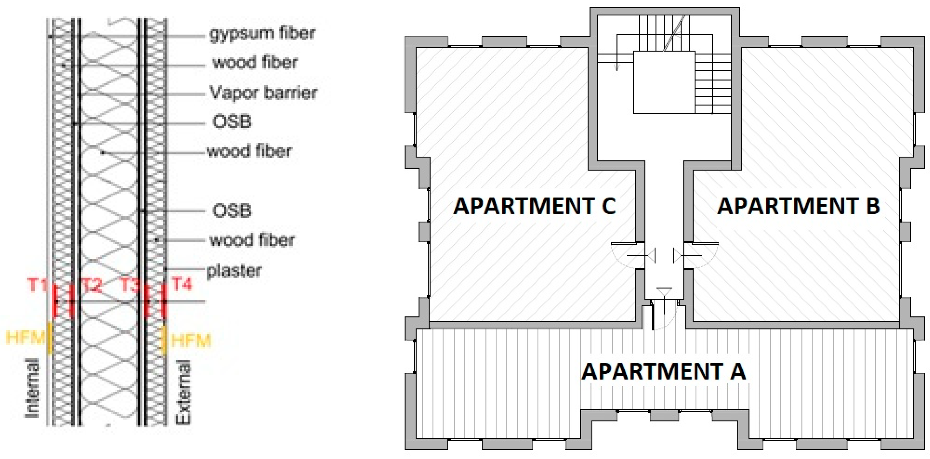
The case study refers to a 5-story social housing building recently built in the province of Trento (Northern Italy, Alpine region). The building has a platform frame structure and a reinforced concrete stairwell. The envelope is composed of highly insulated walls (U = 0.12 W/(m²·K)) and triple-pane low-e windows (U_g = 0.6 W/(m²·K), hemispherical T_sol = 0.43, hemispherical T_vis = 0.66). The heating system consists of a centralized condensing boiler supplying the radiant floor systems and it is controlled by room thermostats. A mechanical ventilation system provides fresh air to the apartments with a constant airflow rate of 0.5 ACH. During the heating period, heat recovery on the exhaust air is implemented, while during the free-floating period, a manual damper at each apartment level is allowed to by-pass the heat recovery. No active cooling is provided during the summertime. The occupants are free to open the windows independently from the mechanical ventilation system operation, both to operate the window roll-up shutters and to modify the thermostat set point.

A weather station close to the monitoring site, whose details are given in [30], collects the weather data every 10 min (dry bulb temperature, relative humidity, wind speed, and solar irradiance on horizontal are specifically used for this study). A monitoring system measures the indoor air temperature every 10 min and the thermal energy delivered daily by the radiant floor system in every apartment, although the latter quantity was not used in the calibration process since it was performed in a free-floating period. In a few apartments, additional sensors were installed, concerning the heat transfer behavior of the external wall (internal and external surface temperatures and heat flow densities, as shown in Figure 1), the indoor air temperature in different rooms, the mechanical ventilation air supply temperature, and the open/closed status of the windows.

For the purpose of this work, an intermediate floor of the building was chosen, where apartments named A, B, and C are identified (Figure 1). Apartment A, as shown in Table 2, is the one equipped with additional probes. As previously mentioned, in order to investigate the impact of the granularity of the metering on the calibration results, two data sets were created (Table 2). The detailed data set, made available to UniTN, includes all the metered quantities concerning the intermediate floor at the highest measurement frequency. The basic data set, provided to the other three research groups, consists of a selection of the metered quantities at a lower time and space resolution. Therefore, the basic data set can be seen as the output of a more essential monitoring system that has been installed in the building.

2.2. Modeling

The building floor and the surrounding buildings were firstly drawn in open studio (Figure 2), and then the geometry was imported in each energy simulation environment. This way, the possible shadows produced by neighboring buildings were taken into account. Clearly, the spatial resolution of the metered quantities influenced the physical modeling, so that the research groups provided with the basic data set adopted a simple thermal zoning, and represented the building floor as two thermal zones, corresponding to the set of the three apartments and to the stairwell (see again Figure 2). In turn, the research group provided with the detailed data set defined fourteen thermal zones, namely five zones in apartment A, and nine zones corresponding to apartments B and C and the stairwell. Internal partitions were neglected by PoliTO, PoliMI, and UniTOV, while they were explicitly modeled by UniTN.

From the yearly meteorological data set, the month of October 2017 was extracted to be used as the calibration period, considering the first week for the conditioning of the building inertia and the remaining 3 weeks for the proper calibration. During October, thanks to the high level of thermal insulation, the heating system was off. The length of the calibration period is in line with the literature, as it can be deduced from the data in the review paper by Chong [26]. By analyzing the calibration studies based on temperature monitoring data, it was found that in 48% of the papers, the calibration period was up to 1 month, while in 72% of the papers, it was up to 2 months.

Subsequently, two further monthly periods where the building remains in free-floating were identified, namely May 2018 and August 2018, which are to be used as validation periods. It may be argued that the climatic conditions in May are more similar to October, while August should provide a more challenging test for the models calibrated in October.

The baseline case models implemented constructions as described in the design documentation and standard internal gain schedules for residential units [31]. Window roll-up shutters were supposed to be in use only during night-time. A constant mechanical ventilation flow rate equal to 0.5 ACH was assigned (ACH_MV = 0.5). In the baseline case models developed by PoliTO, PoliMI, and UniTOV, additional natural ventilation flow rate due to possible windows opening by the occupants was assumed null.

Differently from the others, the baseline case model developed by UniTN benefited from the additional data available in the detailed data set (Table 2). The detailed monitoring showed that in apartment A, the windows are often open during the day, and that the mechanical ventilation air supply temperature is not necessarily equal to the outdoor temperature, as if the occupants did not switch on the heat recovery by-pass. Therefore, in the baseline case model by UniTN, the windows in apartment A are open according to the measured switch signals; a natural ventilation flow rate, additional with respect to the mechanical one, is calculated depending on the wind pressure and the temperature difference, thus following the standard approach [32]. Firstly, the window opening area (A_ow) is estimated according to the measured state of opening, the opening angle evaluated based on the windows sizes, and the occupants’ habits drawn from an interview. An angle of 10 degrees is considered for windows; 20 degrees is considered for French doors; and 90 degrees is considered for the bathroom window.

Then, the airflow rate for natural ventilation is modeled for each room in apartment A, considering the single side impact configuration by Equation (1). This equation is solved in a coupled fashion in Trnsys, which both affects and depends on the internal temperature of the room.

$$AC{H}_{NV}=\frac{1800}{V}·A_{ow}·\sqrt[2]{C_t+C_w·w^2+C_{st}·H·\left|T_i-T_e\right|}$$

(1)

where:

• V is the room air volume in (m³);
• C_t takes into account wind turbulence and is assumed equal to 0.01, according to EN 15242;
• C_w takes into account wind speed and is assumed equal to 0.001, according to EN 15242;
• C_st takes into account stack effect and is assumed equal to 0.0035, according to EN 15242;
• H is the free area height of the window in (m);
• w is the wind speed from weather file in (m/s);
• T_i is the room air temperature in (°C) from the room energy balance;
• T_e is the outdoor air temperature in (°C) from the weather file.

As far as the mechanical ventilation in apartment A is concerned, the measured air supply temperature profile is given as input. Finally, the natural ventilation flow rates in apartments B and C are modeled scaling the corresponding flow rate in apartment A by proper scaling factors, whereby the values are considered as parameters of calibration.

2.3. Performance Metrics

As already discussed in the introduction, in the calibration process, the most frequently metered quantity is energy consumption, and thus, calibration criteria are usually expressed in terms of percentage of discrepancy between measured and simulated consumption. In the present case, where the building is simulated in free-floating, indoor air temperature appears as the most natural quantity to assess the performance of the models. Therefore, the simulated indoor air temperature was compared with the measured one at every time step of the calibration period. The overall agreement between simulation results and measurements on the whole simulation period was evaluated through the root mean squared error, i.e.,

$$RMSE=\sqrt{\frac{{{\displaystyle \sum }}_k{\left(M_k-S_k\right)}^2}{N}}$$

(2)

where M_k and S_k represent the measured and simulated temperature at time step k, respectively, and N is the number of time steps. In the absence of indication form standards and guidelines regarding the maximum acceptable discrepancy in a calibrated model when targeting the indoor temperature rather than the energy consumption, it was decided to adopt a physical limit, namely, the experimental accuracy for the temperature measurement in the monitoring system. Thus, the research groups handling the basic data set (Table 1) considered the model as calibrated if the RMSE referring to the air temperature of the apartments thermal zone was lower than the temperature measurement accuracy ε = 0.5 °C. The research group dealing with the detailed data set (Table 1) defined an RMSE for every thermal zone in apartment A and for apartments B and C, and then calculated a weighted average RMSE considering the zone/apartment volumes. Furthermore, the standard deviation σ among the individual RMSEs, each referring to either an apartment or a room, was used as an additional calibration objective to ensure uniformity of performance.

Finally, correlation plots of the simulated air temperature versus the measured one were drawn, and the R² value of the linear interpolation was used as a simulation performance indicator.

2.4. Manual Calibration with Basic Data Set

PoliTO and PoliMI performed a manual calibration, which was preceded by a sensitivity analysis to the main building envelope parameters, and user behavior parameters are reported in

Table 3. Parameters of the sensitivity analysis performed in the manual calibration approach (base values and range), and range of variation of the parameters in the automatic calibration approach.

	Parameter	Base Value	Variation (Manual)	Variation (Automatic)
envelope	Mineral wool/wood fibers thermal conductivity	λmw = 0.038 W/(m·K) λwf = 0.05 W/(m·K)	+ 5% ÷ + 20%	-
	Thermal bridges	ΨL = 0	ΨL = 5 ÷ 15 W/K	ΨL = 0 ÷ 50 W/K
	Glazings g-value	g = 0.52	g = 0.34 ÷ 0.40	-
	Internal mass	Air capacity multiplier ACM = 1 Partitions surf. Spart = 0 No furniture	ACM = 1 ÷ 10 Spart = 259 m2 ÷ 1034 m2 (to include furniture)	ACM = 1 ÷ 11
occupants	Internal gains schedule	standard (UNI 11300–1, 2014)	(a) Reduced by factor 5% ÷ 50% (b) Modified conserving daily energy gain	Increased or decreased up to 50%
	Solar irradiance threshold for shutters use	Gmin = 1376 W/m2	Gmin = 200 ÷ 300 W/m2	Gmin = 50 ÷ 1000 W/m2
	Natural ventilation flow rate	ACHNV = 0	ACHNV = 0.5 ÷ 1.5 (a) hourly schedule (b) when Text > Tmin	ACHNV = 0 ÷ 1.5 constant

. The envelope parameters considered were as follows: the thermal conductivity of the insulation layers, the thermal bridges overall correction, the g-value of the glazings, and the internal mass. The latter, including the furniture, was modeled in the following different ways: through a multiplier of the indoor air volume capacity (ACM) as suggested in [33], and/or by introducing explicitly internal partitions. Regarding the occupants, the following parameters were considered: the internal gains daily profile, the use of roll-up shutters also during the day for solar shading when a minimum solar irradiance on the window is reached, and the natural ventilation flow rate resulting from the windows opening. The latter was modeled using the following two approaches: opening according to a daily schedule or opening when outside air temperature reaches a given threshold. In both cases, opening the windows determines the given ACH_NV, which is then added to the ACH_MV. In other words, a deterministic model of the occupants’ operation of the shadings and of the windows was chosen, either in the simplest form of a time schedule or by implementing a deterministic rule.

The parameters were varied one-at-a time and the sensitivity was evaluated by means of a sensitivity index s:

$$s=\frac{\Delta O}{\raisebox{1ex}{$\Delta I$}\!\left/ \!\raisebox{-1ex}{$I_m$}\right.}$$

(3)

where O and I are the output (indoor air temperature) and the input (parameter), respectively, ΔO represents the root mean squared variation of the outputs with respect to the baseline case value at every time step k, as in Equation (4):

$$\Delta O=\sqrt{\frac{{{\displaystyle \sum }}_{k=1}^N{\left(O_k-O_{bk}\right)}^2}{N}}$$

(4)

while ∆I/I_m represents the variation of the input with respect to the baseline value, which is normalized by the average input as in Equation (5):

$$\frac{\Delta I}{I_m}=\frac{I-I_b}{I_m}$$

(5)

In Equations (3)–(5) the subscript m indicates the mean value and the subscript b indicates the baseline value. It has to be mentioned that in the case of natural ventilation, I is set as equal to the total air changes, namely the sum of ACH_MV and ACH_NV, so that I_b = ACH_MV = 0.5, since in the baseline case, the windows are assumed to be closed. Different forms of sensitivity indexes, either dimensional or not, can be found in the literature related to building energy simulations [34]. The sensitivity index s proposed by the authors is a revised version where the input variation is normalized by the mean value, so that sensitivities to different quantities can be compared, but the output variation is not normalized. Actually, using a normalized output ∆O⁄O_m for the environmental temperature possibly leads to very small values, hardly distinguishable from each other’s. Following sensitivity analysis, the most influential parameters were combined and adjusted in order to reach the calibration target.

2.5. Automatic Calibration with Basic Data Set

UniTOV performed an automatic calibration by coupling IDA ICE with the optimization engine GenOpt, through the parametric runs macro. The authors also used this approach in case of existing/historical buildings, where indoor climate variables (i.e., temperature and relative humidity) were collected over time [35,36]. The objective function was identified in the RMSE for the apartments thermal zone, which is defined in (1). Since automatic calibration enables an easy variation of the parameters compared to manual calibration, this potential was exploited. More in detail, the 3 steps of the internal gains scheduled from the standard [31], namely 11 p.m.–7 a.m., 7 a.m.–5 p.m., and 5 p.m.–11 p.m., were allowed to vary, possibly leading to a profile that was very different from the base one. Moreover, the possibility that the threshold for shutter activation depended on the window orientation was tested. The range of varied parameters is reported in Table 3.

2.6. Automatic Calibration with Detailed Data Set

UniTN benefited from the detailed monitoring data of the external walls and adopted a multi-stage calibration process. First, the thermal properties of the wall layers were calibrated by performing a simulation at the single-wall level as in [15]. The wall response in terms of inside and outside heat flow densities under imposed surface temperatures (equal to measured profiles in October 2017) was simulated. The wall properties were then optimized in order to reproduce the measured heat flow densities on both sides and the calibrated wall models were implemented in the baseline model of the building floor. At this stage, the calibration procedure based on the optimization of RMSE and a penalty function was followed [12], due to the availability of design documentation and material certificates. The penalty function (P) is calculated as the sum of the individual penalty functions of each j-th calibrated material property (v_j), by penalizing values that deviate too far from the value declared in the data sheets (IG_j). Therefore, a Gaussian distribution of variance Var²_j around the IG_j value of each individual property is considered. The overall penalty function will then be as follows:

$$P={\displaystyle \sum }_j\frac{1-exp\left(-\frac{v_j-I{G}_j}{2Va{r}_j^2}\right)}{\sqrt{2Va{r}_j^2}}$$

(6)

As a second step, multi-objective automatic calibration on the baseline model was carried out using a custom optimization algorithm based on a generation-based control approach driven by a MARS meta-model [37]. Besides internal gain’s profiles, the calibration parameters involved the threshold irradiance for shutter’s activation for each apartment, the indoor air volume capacitance multiplier, the windows opening angle in apartment A, and the scaling factors for natural ventilation flow rates for apartments B and C. Finally, among the Pareto front solutions, a single solution was selected through a post-Pareto analysis described in Equation (7):

$$\underset{i \in Pareto}{\min }\left\{0.7\frac{RMS{E}_i}{\underset{i \in Pareto}{\max }\left(RMS{E}_i\right)}+0.3\frac{{\sigma }_i}{\underset{i \in Pareto}{\max }\left({\sigma }_i\right)}\right\}$$

(7)

where the first index measures the overall root mean square error (RMSE_i) evaluated as a volume-weighted average of the RMSEs of individual rooms/apartments and normalized against the maximum value among the solutions of the Pareto front. On the other hand, the second index looks at the standard deviation (σ_i) between the different RMSEs trying precisely to also minimize the values of the individual rooms that weigh less in the first index because of the lower room volume. The choice of weights was made to consider the differences in importance of the two indices.

2.7. Validation and Revision

The calibrated models obtained by each group were tested on two further monthly periods, namely May and August 2018. The minimum, average, and maximum dry bulb temperature as well as the average daily solar irradiation on a horizontal surface during the calibration month and the validation months are reported in

Table 4. Climatic parameters in the calibration month (October 2017) and in the validation ones (May and August 2018) for the case study.

	Dry Bulb Temperature—min, Average, Max (°C)	Daily Solar Irradiation on Horizontal—Average (kWh/m2)
October 2017	4.0–13.9–23.6	2.93
May 2018	9.3–17.9–29.9	4.65
August 2018	12.2–24.2–35.7	5.40

, in order to highlight similarities and differences in the climatic conditions. It may be observed that both May and August are warmer than October, but May conditions are more similar to it. Therefore, validation in May is expected to be less challenging than in August.

3. Results

3.1. Baseline Models Results

The apartments indoor air temperature during the third week of October obtained from the baseline model simulations is reported in Figure 3, together with the measured profile. In the case of the more detailed baseline model developed by UniTN, the indoor temperature is obtained as the weighted average of the various thermal zones, in which apartments A, B, and C are subdivided. The RMSE calculated over the calibration period for each baseline model is reported in

Table 5. Baseline model’s performance (October 2017).

Research Group	Tool	RMSE (°C)
PoliTO	EnergyPlus 9.4	1.8
PoliMI	TRNSYS 17	1.8
UniTOV	IDA ICE 4.8	1.6
UniTN	TRNSYS 17	1.5

. It can be noticed that the outputs from the different simulation tools are generally coherent with each other. Compared with the measured profile, they all capture the weekly trend, but they overestimate the indoor air temperature mean value and variation amplitude; moreover, they anticipate the peaks. By comparing the outputs from PoliTO, PoliMI, and UniTOV, who adopted a common modeling approach with respect to thermal zones, it can be derived that using different simulation tools does not lead to relevant discrepancies. On the contrary, UniTN and PoliMI adopted the same simulation tool, i.e., TRNSYS, while implementing different modeling approaches, specifically, a detailed and a simplified one, respectively. In this regard, Figure 3 shows that the simulation output by UniTN is generally damped, especially in the warm peaks, with respect to the output obtained by PoliMI. This outcome can be attributed to the inertia of the partition walls that are modeled in the base case by UniTN, but they are not considered by PoliMI and the other groups. In general, Table 5 shows that the baseline model simulations do not match with the measured data within the probe’s measurement uncertainty; therefore, none of the baseline models can be considered acceptable.

3.2. Manual Calibration Results

The sensitivity analysis performed by PoliTO and PoliMI showed a modest influence of the external opaque envelope parameters, namely, the thermal conductivity of the insulation layers and the thermal bridges correction. On the contrary, reducing the glazing solar heat gain coefficient, introducing external solar shading, reducing/modifying the internal gains profile, adding internal mass, and introducing natural ventilation during the day all have an impact on the simulation output. An example is shown in Figure 4, where the variation in the indoor air temperature profile during the third week of October 2017 for some parametric variations brought to the base model is reported (PoliTO-EnergyPlus simulations). The negligible impact of an increase by 20% of the thermal conductivity of the insulation layers can be noticed, while reducing the window’s g-value or the threshold for activating the shutters to 300 W/m² significantly helps to lower the temperature peaks, although the shape of the curves is still different from the measured one. For every parameter varied according to Table 3, many values were considered, and thus, many sensitivity index values calculated as in Equation (3) were achieved. For the sake of simplicity, for each parameter varied, the maximum sensitivity index was identified and reported in Figure 5 (PoliMI-TRNSYS simulations).

The combination of the most influential variations resulted in several acceptable solutions, listed in

Table 6. Calibrated models by PoliTO, PoliMI, and UniTOV.

	Model	Internal Mass	Thermal Bridges Correction	Natural Ventilation	Internal Gains a	Solar Shading Activation Threshold	RMSE (°C)
PoliTO-EnergyPlus	PoliTO 1	ACM = 5 Spart Spart = 259 m2	-	ACHNV = 0.5 1 p.m.–10 p.m.	-	300 W/m2	0.5
	PoliTO 2	ACM = 5 Spart = 259 m2	-	ACHNV = 0.5 1 p.m.–10 p.m.	Profile PoliTO	300 W/m2	0.4
	PoliTO 3	ACM = 8 Spart = 0	-	ACHNV = 0.5 1 p.m.–10 p.m.	Profile PoliTO	300 W/m2	0.4
	PoliTO 4	ACM = 5 Spart = 259 m2	-	ACHNV = 0.5 11 a.m.–9 p.m.	Profile PoliTO	300 W/m2	0.4
PoliMI-TRNSYS	PoliMI 1	ACM = 5 Spart = 259 m2	-	-	-	200 W/m2	0.5
	PoliMI 2	ACM = 3 Spart = 1034 m2	-	-	-	200 W/m2	0.5
	PoliMI 3	ACM = 5 Spart = 259 m2	-	ACHNV = 0.5 1 p.m.–10 p.m.	-	300 W/m2	0.5
	PoliMI 4	ACM = 5 Spart = 259 m2	-	ACHNV = 1.5 if Text > 18 °C	-	200 W/m2	0.5
	PoliMI 5	ACM = 3 Spart = 1034 m2	-	ACHNV = 1.5 if Text > 16 °C	Base reduced by 25%	-	0.4
	PoliMI 6	ACM = 3 Spart = 1034 m2	-	ACHNV = 0.5 1 p.m.–10 p.m.	Base reduced by 25%	-	0.4
UniTOV-IDA ICE	UniTOV	ACM = 11	Ψ∙L = 0.32 W/K	ACHNV = 0.08	Profile UniTOV	350 W/m2 N 65 W/m2 E 611 W/m2 S 64 W/m2 W	0.3

^a Internal gain’s profiles are presented in Figure 7.

, named PoliTO 1–4 and PoliMI 1–6, which were obtained with a minimum of two and a maximum of four variations together. It can be noticed that all of the solutions require the modeling of additional internal mass, either through a lumped capacity approach applied to the air volume (ACM) or through an explicit simulation of internal partitions (S_part). The indoor air temperature variation in the third week of October obtained by some of the calibrated models is shown in Figure 6, for a comparison with the measured profile and with the baseline case’s simulation profiles reported in Figure 4.

3.3. Automatic Calibration/Basic Data Set Results

The automatic calibration performed by UniTOV using IDA-ICE resulted in a calibrated model with a very good agreement with measured data, namely, RMSE = 0.3 °C. The calibrated parameters are shown again in Table 6: the air capacity multiplier is set to 11, a modest thermal bridges correction is applied, and a small amount of natural ventilation (0.08 h⁻¹) is added to the base mechanical ventilation rate (0.5 h⁻¹). The internal gain’s profile is modified with respect to the base one, according to a profile named UniTOV, and it is shown in Figure 7 together with those resulting from the calibrations performed by the other groups. Different solar irradiance thresholds for shutter’s activation are actually found for different orientations of the windows. The small threshold irradiances resulting from calibration for the east and west orientation suggest that shutters are used primarily on these facades.

3.4. Automatic Calibration/Detailed Data Set Results

The calibration of the thermal properties of the external walls (

Table 7. UniTN-TRNSYS calibration of the external wall: base and calibrated properties.

	Base Properties			(Calibrated–Base)/Base
s cm	ρ kg/m3	c J/(kg·K)	λ W/(m·K)	Δρ (%)	Δc (%)	Δλ (%)
6	160	2100	0.050	−29	−3	1
1.8	550	1221	0.098	−56	7	−2
18	40	1030	0.038	−9	−12	−2
1.8	550	1221	0.098	−56	7	−2
6	50	2100	0.038	−27	1	0
1.5	1200	1100	0.320	−47	−5	0

), which was obtained from single-wall level analysis, resulted in a negligible modification of the thermal conductivities of the layers, so that the U-value of the wall remains equal to 0.12 W/(m².K). The reduction in the material’s density with respect to the base values appears more significant, although the latter already allows for the classification of the wall as a “light” one.

The automatic calibration at the building level resulted in the model described in

Table 8. UniTN-TRNSYS calibration of the building model: parameters range and calibrated values.

	Range	Calibrated
Solar irradiance shading closed Ap. A	200–1400 W m−2	200 W m−2
Solar irradiance shading closed Ap. B	200–1400 W m−2	300 W m−2
Solar irradiance shading closed Ap. C	200–1400 W m−2	1400 W m−2
Solar irradiance difference shading closed–open Ap. A	0–200 W m−2	200 W m−2
Solar irradiance difference shading closed–open Ap. B	0–200 W m−2	200 W m−2
Solar irradiance difference shading closed–open Ap. C	0–200 W m−2	50 W m−2
Window opening angle Ap. A. Zone KS	10–90 deg	10 deg
Window opening angle Ap. A. Zone WC	10–90 deg	40 deg
Window opening angle Ap. A. Zone LS	10–90 deg	10 deg
Window opening angle Ap. A. Zone LM	10–90 deg	10 deg
ACHNV Ap. B/Ap. A	0–1.5	0.5
ACHNV Ap. C/Ap. A	0–1.5	0
ACHMV	0.5–0.65	0.55
Stairwell zone infiltration ACH	0.1–0.6	0.3
(Tsupply–Text) Ap. B/Ap. A	0.5–1.5	0.5
(Tsupply–Text) Ap. C/Ap. A	0.5–1.5	0.5
Time shift internal gains profile compared to base profile	−2–+2 h	−1.167 h
Morning gain amplification living area	0.5–1.5	1.1
Afternoon gain amplification living area	0.5–1.5	1.3
Evening gain amplification living area	0.5–1.5	0.5
Morning gain amplification sleeping area	0.5–1.5	0.7
Afternoon gain amplification sleeping area	0.5–1.5	1.3
Evening gain amplification sleeping area	0.5–1.5	1.5
Air capacity multiplier	1–5	2.25

. It is worth noticing that in the calibrated model, the shutters are activated at different thresholds for the three apartments. Moreover, in apartment B, the natural ventilation flow rates are half that of the apartment A flow rates, while in apartment C, the windows are generally closed. The overall performance of the calibrated model, in terms of the mean floor air temperature, is RMSE = 0.5 °C.

3.5. Validation and Revision Results

The performances of the calibrated models in the two validation periods of May and August 2018 are shown in Figure 8, where the performances during the calibration period are also reported in order to ease the comparison. In general, as it can be expected, all the calibrated models performed worse in the validation periods, with an RMSE generally greater than the threshold representing the measurement uncertainty. While the mismatch with respect to the measured data remains somehow limited in May, it becomes dramatic in most of the cases in August. It can be noticed that among the manually calibrated models, the ones named PoliMI 4 and PoliMI 5 are less prone to decreases in their performances in both validation periods. By inspecting the model’s settings in Table 6, it is found that they are the only models where the natural ventilation flow rates are provided through a deterministic rule, rather than in terms of constant or hourly variable values. The models obtained through the automatic calibration process appear robust as long as the validation period is relatively similar to the calibration one, yet they will not necessarily perform well in August, as the case of the UniTOV model shows. The more sophisticated model by UniTN, implementing a detailed thermal zoning approach as well as benefitting from the detailed measurement data set, also performs well in August. However, its performances are similar to the simpler model PoliMI4.

The results of the validation process led the research groups who obtained unsatisfactory results to revise the models calibrated in October, with the idea that the occupants’ behavior was not properly captured by the previous approaches.

PoliTO decided to implement a deterministic rule for natural ventilation during the daytime, based on a minimum and maximum outdoor air temperature (equal to 16 °C and 27 °C, respectively): when the air temperature is between them, ACH_NV is set as equal to 2, otherwise it is set to 1, and during the night it remains equal to 0.5. At the same time, the solar irradiation threshold for activating the shutters during the day was set to 200 W/m² (PoliTO 5) or 300 W/m² (PoliTO 6). As is shown in

Table 9. Performance of the revised models.

Model	Internal Mass	Thermal Bridges Corr.	Natural Ventilation	Internal Gains	Solar Shading Activation Threshold	Oct. RMSE (°C)	May RMSE (°C)	August RMSE (°C)
PoliTO 5	ACM = 5 Spart = 259 m2	-	11:00 a.m.–11:00 p.m. ACHNV = 1.5 if 18 °C < Text < 26 °C	Profile PoliTO	200 W/m2	0.6	0.5	3.0
PoliTO 6	ACM = 5 Spart = 259 m2	-	11:00 a.m.–11:00 p.m. ACHNV = 1.5 if 18 °C < Text < 26 °C	Profile PoliTO	300 W/m2	0.5	0.6	3.8
UniTOV 2	ACM = 11	Ψ∙L = 0.32 W/K	ACHNV = 0.81	Profile UniTOV 2	528 W/m2 N 53 W/m2 E 53 W/m2 S 53 W/m2 W	-	-	0.5

, the revised models by PoliTO perform in an acceptable way in both October and May, with PoliTO 5 performing better in May and PoliTo 6 performing better in October, suggesting that the threshold for the shutter’s activation should be adjusted monthly or seasonally. Yet, they both maintain an important discrepancy with the measured data during August.

In parallel, UniTOV decided to repeat the automatic calibration on August, allowing all the parameters used in the calibration of October to vary again. This exercise led to the parameter’s setting, shown in Table 9, for the model named UniTOV 2. By comparison with Table 6, the parameters related to the building envelope, although they were allowed to vary, reached the same calibration values, while all the parameters related to the occupants reached different values. In particular, a higher natural ventilation flow rate, a new internal gains profile with lower values during the central hours of the day and the evening hours and, remarkably, a lower threshold for activating the shutters on the South façade were all obtained. It has to be remarked that the revised models are all reported in Table 9 for the sake of simplicity, but while the models PoliTO5 and PoliTO6 were achieved by manual calibration addressing October, May, and August, the model UniTOV2 resulted from an automatic calibration, specifically during August.

3.6. Windows Opening Monitoring Results

Since the calibrated models obtained differ from each other mainly because of the parameters related to the occupants’ behavior, it is worth presenting the only measurements included in the detailed data set that refer to it, namely, the operation of the windows in apartment A (again, see Table 2). Figure 9 shows the fractions of the time when at least one of the windows in each room of the apartment is open in the three periods of interest. The behaviors are quite unexpected considering the presence of a mechanical ventilation system. These figures seem to point to a lack of knowledge of how the building works combined with a rebound effect related to the high energy efficiency of the building. The operation of the windows by the occupants appears to be quite different in the three months and in the various rooms. With the remarkable exception of the living room, which includes the kitchen and where windows are frequently open in every season, windows are closed most of the time in October, and they are open most of the time in August, with an intermediate situation in May.

By looking more in detail to the different time frames of the day and to the different rooms, it can be noticed that the habit of keeping the windows open in the bedrooms during the late afternoon and evening hours (time frame from 5:00 p.m. to 10:00 p.m.) starts in May and extends to the night hours (from 10:00 p.m. to 6:00 a.m.) in August. This behavior can clearly be interpreted as a comfort ventilation strategy implemented by the occupants to mitigate the warm climatic conditions in the absence of an active cooling system.

4. Discussion

4.1. Comparison among Tools

The possible impact of the different BES tools can be analyzed by comparing the results obtained by the three research groups who had access to the same basic data set and shared the same modeling approach in terms of thermal zoning and ventilation, namely PoliTO (EnergyPlus), PoliMI (TRNSYS), and UniTOV (IDA ICE). The base models behave in a very similar way, as shown in Table 5 and Figure 3, since the RMSEs are all comprised between 1.5 °C and 1.8 °C. In fact, given that the building is simulated in free-floating, the potential differences among the tools are limited mainly to the processing of solar radiation data and to the modeling of the heat transfer across the components of the building envelope.

4.2. Manual Versus Automatic Calibration

Some considerations regarding the advantages of automatic calibration over manual can be derived by comparing the results obtained on the one side by UniTOV (automatic calibration) and on the other side by PoliTO and PoliMI (manual calibration). These three models are chosen because they are all based on the basic data set (Table 1). As the very low RMSE = 0.3 °C achieved by the UniTOV calibrated model demonstrates (Table 6), an automatic calibration can be more effective than a manual one in terms of reaching a more accurate matching with the measured data, even though it manages more parameters (e.g., different thresholds for shutter’s activation rather than a unique) and thus obtains a more detailed model. Moreover, this effectiveness of the automatic calibration process enabled an easy refinement of the model, after testing its performance in May and August, as it was reported in Section 3.6. It has to be remarked that a direct comparison of the workload in the performing manual and automatic calibration was not carried out in the present study; however, to the authors’ experiences, the workload is usually heavily reduced through automation, which also allows the evaluation of a higher number of scenarios [7].

4.3. Basic Versus Detailed Data Set

The performance in October of the calibrated model obtained by UniTN is similar to that of the other calibrated models (Figure 8). From this point of view, it appears that having access to detailed monitoring does not guarantee a better calibration. In particular, the detailed monitoring of the external wall, providing, in principle, precious information, did not lead to significant modifications of the corresponding thermal properties with respect to the design ones (Table 7). This outcome is coherent with the fact that the other simulations models also proved to be poorly sensitive to the building envelope properties (Figure 5).

Indeed, the relatively good overall performance of the UniTN calibrated model is the result of the combination of a very good performance in predicting the temperature in apartment A (the one with detailed monitoring) and a less good performance in predicting the air temperature in apartments B and C. These different performances are shown in (Figure 10), where the simulated temperature is correlated to the measured one for apartment A (R² = 0.7135) and apartment B (R² = 0.579). This means that monitoring the opening of windows is useful, but it should be extended to most of the building users to guarantee an excellent quality of the calibration as a whole. Moreover, it suggests that in the calibration of a well-insulated building, it is more important to monitor the users’ behavior than the heat transfer across the building envelope.

By looking at the validation results (Figure 6), it seems that having access to detailed monitoring data leads to a more robust calibrated model, namely, performing well outside the calibration month. Yet, as already mentioned, this may also be the case of a model developed with access only to limited data (PoliMI 4).

4.4. Validation and Users’ Behaviour

As expected, since calibration is an ill-posed inverse problem with many unknown parameters, multiple calibrated solutions are obtained. Each of them could be considered an acceptable representation of the building and its use under the boundary conditions acting during the chosen calibration period. In this regard, the validation phase proves to be crucial because (a) it helps discriminating among the different solutions, identifying the more robust ones (e.g., PoliMI 4 and PoliMI 5 among the PoliMI ones) and (b) it highlights the necessity to refine them. It has to be noticed that the choice of the validation period is critical because if in the latter, the boundary conditions are too similar to the calibration period (e.g., May versus October), the validation phase fails to detect the weak points of a model (Figure 8).

In this case study, the weak points of the calibrated models concern the users’ actions. The occupants are adaptive actors of the building, changing their habits according to the climatic conditions, especially in the absence of active systems. High performance buildings are characterized by a non-negligible impact of occupants on energy demand. Hence, an incorrect modeling of users’ behaviors during the calibration can lead to an over-calibration of the other parameters. Nonetheless, those parameters that are related to the occupants (internal gains profile and operation of the windows and of the roll-up shutters) can, in principle, vary from season to season. Consequently, the validation phase naturally leads to a revision of the calibration models, thus aiming to improve their flexibility and capability to capture the variations of the users’ actions.

4.5. Reproducibility

If the final parameters of the models calibrated by the four groups (Table 6, Table 7 and Table 8) are compared, it is possible to notice both some similarities and discrepancies. Starting from the common features, all the models are characterized by an additional internal mass with respect to the mere indoor air volume mass; although, this additional mass is either modeled explicitly in terms of partitions or implicitly in terms of fictitious air mass. Moreover, in the calibrated models, the building envelope thermal properties are either unmodified with respect to the baseline case (PoliMI and PoliTO) or only marginally modified (UniTOV introduced a correction for thermal bridges, which results in increasing transmission losses by less than 1%; UniTN varied the layer’s properties without changing the wall thermal transmittance). In every calibrated model, it is found that solar shading systems are active during the day, although the thresholds for activation may differ from model to model. As far as the internal gain’s profile is concerned, it can be noticed that calibrated profiles by PoliMI, UniTOV, and UniTN, although different (Figure 7), all result in a 24–25% reduction on the daily energy gain with respect to the base profile. In turn, additional air changes related to the opening of the windows are found in each calibrated model. The apparently small value of the natural ventilation flow rate in the UniTOV model (ACH_NV = 0.08 h⁻¹, Table 6) is indeed coherent with the higher ventilation flow rates in the other models (Table 6 and Table 8), since in the latter, they are concentrated in a part of the day, while in the former, they are considered active all day long.

In the end, it can be stated that the calibration process carried out in parallel by the four groups led to partially coherent results. The models are obviously different, starting from their settings, but the changes that were applied to the baseline models in order to match the measurements data mostly point in the same directions. The following question then arises, which must be addressed in a future development of the present study: to what extent does using differently calibrated models to design retrofit or management interventions lead to different conclusions?

5. Conclusions and Prospects

A BES model calibration exercise was performed in parallel by different research groups, adopting either manual or automatic calibration, with access to basic or detailed monitoring data, and using different simulations tools. It was found that, despite these differences in the calibration settings, the calibrated models obtained by the different groups are characterized by a certain degree of coherence, in terms of the building’s envelope properties, internal gain’s profiles, solar shading strategies, and users’ operation of the windows.

It was found also that calibrated models can perform in an unsatisfactory way outside the calibration period (RMSEs in May and August are between 1.1 and 10.8 times the corresponding RMSE in October), and thus, it is recommended to identify at least another period, which is similar but at the same time challenging, to validate the calibrated models. The validation phase was sorted in the rejection of the models with the worst performance and in the revision/refinement of the most promising ones. In the present case study, the weak points of the calibrated models worthy of a revision refer to the users’ actions, namely, the internal gain’s profiles and the modeling of the operation of the roll-up shutters and of the windows.

In the present study, the calibration is limited to the thermal behavior of the building envelope and the users’ operation in free-floating periods of the year. If the final purpose of developing and calibrating a simulation model of an existing building is evaluating the impact of various retrofit interventions on energy consumption, the calibration should also involve the HVAC system model and the users’ behavior in the heating or cooling season, which could be a further development of the present study. With a view of calibrating the BES models in different periods, the advantage offered by an automatic calibration approach in easily managing the multi-parametric nature of the problem has to be taken into account. An expert user can guarantee the effectiveness of the automatic procedure; otherwise, the lack of control in such a system would determine an increase in erroneous outputs. To overcome this issue, the human–computer interaction is showing to be an encouraging technique to be used in the near future. It would allow for the development of user-centered building performance simulation systems that would also provide the non-expert user with a conscious performing of his/her task [38].

The model calibrated by UniTN also resulted in a relatively good also in the validation periods. Thus, it can be inferred that having access to detailed monitoring data, besides orientating the development of the building model, leads to more robustly calibrated models. Among the detailed information, it was found that, at least for a highly insulated building analyzed in free-floating conditions, the monitoring data regarding the heat transfer of the building envelope components are less important than the data regarding the users’ actions, as the BES model proved to be less sensitive to the former than to the latter. At the same time, users’ behavior is characterized by diversity, so that it was found that observations on a single apartment cannot be simply transposed to the others, and data on users’ actions should refer to sufficiently large samples.

As the calibration in this study referred to the free-floating operation of the building, the performance of the model was evaluated in terms of its capability to predict the indoor temperature profile, rather than energy consumption. Since the current guidelines concerning calibration identify the maximum acceptable discrepancy values to consider the model calibrated only in terms of energy, in this paper, the physical threshold of the accuracy of the temperature measurement was adopted. Further efforts could be devoted to identify less strict thresholds for indoor temperatures, possibly discussing the impact in terms of predicted thermal comfort.

References

1. ENEA. Certificazione energetica degli edifici. In Rapporto Annuale 2021; ENEA: Paris, France, 2021. (In Italian) [Google Scholar]
2. ASHRAE. Guideline 14:2002. In Measurement of Energy and Demand Saving; ASHRAE: Peachtree Corners, GA, USA, 2002. [Google Scholar]
3. Coakley, D.; Raftery, P.; Keane, M. A review of methods to match building energy simulation models to measured data. Renew. Sustain. Energy Rev. 2014, 37, 123–141. [Google Scholar] [CrossRef] [Green Version]
4. Fabrizio, E.; Monetti, V. Methodologies and advancements in the calibration of building energy models. Energies 2015, 8, 2548–2574. [Google Scholar] [CrossRef] [Green Version]
5. Huerto-Cardenas, H.; Leonforte, F.; Aste, N.; Del Pero, C.; Evola, G.; Costanzo, V.; Lucchi, E. Validation of dynamic hygrothermal simulation models for historical buildings: State of the art, research challenges and recommendations. Build. Environ. 2020, 180, 107081. [Google Scholar] [CrossRef]
6. Reddy, T.A. Literature review on calibration of building energy simulation programs: Uses, problems, procedure, uncertainty, and tools. ASHRAE Trans. 2006, 112, 226–240. [Google Scholar]
7. Cornaro, C.; Bosco, F.; Lauria, M.; Puggioni, V.A.; De Santoli, L. Effectiveness of Automatic and Manual Calibration of an Office Building Energy Model. Appl. Sci. 2019, 9, 1985. [Google Scholar] [CrossRef] [Green Version]
8. Heo, Y.; Choudhary, R.; Augenbroe, G. Calibration of building energy models for retrofit analysis under uncertainty. Energy Build. 2012, 47, 550–560. [Google Scholar] [CrossRef]
9. Muehleisen, R.T.; Bergerson, J. Bayesian Calibration-What, Why and How. In Proceedings of the International High Performance Buildings Conference, Lafayette, IN, USA, 11–14 July 2016; Paper 167. Available online: http://docs.lib.purdue.edu/ihpbc/167 (accessed on 1 April 2022).
10. Heo, Y.; Augenbroe, G.; Choudhary, R. Quantitative risk management for energy retrofit projects. J. Build. Perform. Simul. 2012, 6, 257–268. [Google Scholar] [CrossRef]
11. Reddy, T.A.; Maor, I.; Panjapornpon, C. Calibrating Detailed Building Energy Simulation Programs with Measured Data—Part I: General Methodology (RP-1051). HVACR Res. 2007, 13, 221–241. [Google Scholar] [CrossRef]
12. Prada, A.; Gasparella, A.; Baggio, P. A robust approach for the calibration of existing buildings models. In Proceedings of the BS2019 16th Int. Building Simulation Conference, Roma, Italy, 2–4 September 2019. [Google Scholar]
13. Cacabelos, A.; Eguía, P.; Febrero, L.; Granada, E. Development of a new multi-stage building energy model calibration methodology and validation in a public library. Energy Build. 2017, 146, 182–199. [Google Scholar] [CrossRef]
14. Pachano, J.E.; Bandera, C.F. Multi-step building energy model calibration process based on measured data. Energy Build. 2021, 252, 111380. [Google Scholar] [CrossRef]
15. Angelotti, A.; Martire, M.; Mazzarella, L.; Pasini, M.; Ballarini, I.; Corrado, V.; De Luca, G.; Baggio, P.; Prada, A.; Bosco, F.; et al. Building Energy Simulation for Nearly Zero Energy Retrofit Design: The Model Calibration. In Proceedings of the 2018 IEEE International Conference on Environment and Electrical Engineering and 2018 IEEE Industrial and Commercial Power Systems Europe, Palermo, Italy, 12–15 June 2018; pp. 1–6. [Google Scholar] [CrossRef]
16. Cozza, S.; Chambers, J.; Brambilla, A.; Patel, M.K. In search of optimal consumption: A review of causes and solutions to the Energy Performance Gap in residential buildings. Energy Build. 2021, 249, 111253. [Google Scholar] [CrossRef]
17. Calì, D.; Osterhage, T.; Streblow, R.; Müller, D. Energy performance gap in refurbished German dwellings: Lesson learned from a field test. Energy Build. 2016, 127, 1146–1158. [Google Scholar] [CrossRef]
18. Hoes, P.; Hensen, J.L.M.; Loomans, M.G.L.C.; de Vries, B.; Bourgeois, D. User behaviour in whole building simulation. Energy Build. 2009, 41, 295–302. [Google Scholar] [CrossRef] [Green Version]
19. Csoknyai, T.; Legardeur, J.; Akle, A.A.; Horvath, M. Analysis of energy consumption profiles in residential buildings and impact assessment of a serious game on occupants’ behaviour. Energy Build. 2019, 196, 1–20. [Google Scholar] [CrossRef]
20. Yan, D.; Hong, T.; Dong, B.; Mahdavi, A.; D’Oca, S.; Gateani, I.; Feng, X. IEA EBC Annex 66: Definition and simulation of occupant behaviour in buildings. Energy Build. 2017, 156, 258–270. [Google Scholar] [CrossRef] [Green Version]
21. Yan, D.; O’Brien, W.; Hong, T.; Feng, X.; Gunay, H.B.; Tahmasebi, F.; Mahdavi, A. Occupant behavior modeling for building performance simulation: Current state and future challenges. Energy Build. 2015, 107, 264–278. [Google Scholar] [CrossRef] [Green Version]
22. Gaetani, I.; Hoes, P.J.; Hensen, J.L.M. Occupant behaviour in building energy simulation: Toward a fit-for-purpose modeling strategy. Energy Build. 2016, 121, 188–204. [Google Scholar] [CrossRef]
23. Zhang, Y.; Bai, X.; Mills, F.P.; Pezzey, J.C.V. Rethinking the role of occupant behaviour in building energy performance: A review. Energy Build. 2018, 172, 279–294. [Google Scholar] [CrossRef]
24. Gaetani, I.; Hoes, P.-J.; Hensen, J.L.M. A stepwise approach for assessing the appropriate occupant behaviour modelling in building performance simulation. J. Build. Perform. Simul. 2020, 13, 362–377. [Google Scholar] [CrossRef]
25. Fabi, V.; Andersen, R.V.; Corgnati, S.; Olesen, B.W. Occupants’ window opening behaviour: A literature review of factors influencing occupant behaviour and models. Build. Environ. 2012, 58, 188–198. [Google Scholar] [CrossRef]
26. Chong, A.; Gu, Y.; Jia, H. Calibrating building energy simulation models: A review of the basics to guide future work. Energy Build. 2021, 253, 111533. [Google Scholar] [CrossRef]
27. Janssen, H.; Roels, S.; Van Gelder, L.; Das, P. Annex 55, Reliability of Energy Efficient Building Retrofitting–Probability Assessment of Performance and Cost (RAP-RETRO)—Probabilistic Tool; International Energy Agency: Paris, France, 2015. [Google Scholar]
28. Kersken, M.; Strachan, P. Building Energy Performance Assessment based on In-Situ Measurements Description and Results of the Validation of Building Energy Simulation Programs; Annex 71 Report; IEA EBC: KU Leuven, Belgium, 2021. [Google Scholar]
29. Angelotti, A.; Ballabio, M.; Mazzarella, L.; Cornaro, C.; Parente, G.; Frasca, F.; Prada, A.; Baggio, P.; Ballarini, I.; De Luca, G.; et al. Dynamic Simulation of existing buildings: Considerations on the Model Calibration. In Proceedings of the Building Simulation Conference Proceedings, Loughborough, UK, 21–22 September 2020. [Google Scholar] [CrossRef]
30. Giovannini, L.; Zardi, D.; De Franceschi, M. Characterization of the Thermal Structure inside an Urban Canyon: Field Measurements and Validation of a Simple Model. J. Appl. Meteorol. Clim. 2013, 52, 64–81. [Google Scholar] [CrossRef]
31. UNI/TS 11300-1; Energy Performance of Buildings Part 1: Evaluation of Energy Need for Space Heating and Cooling. UNI: Milano, Italy, 2014.
32. EN 15242; Ventilation for Buildings–Calculation Methods for the Determination of Air Flow Rates in Buildings Including Infiltration. CEN: Brussels, Belgium, 2007.
33. EN ISO 52016-1; Energy Performance of Buildings–Energy Needs for Heating and Cooling, Internal Temperatures and Sensible and Latent Heat Loads—Part 1: Calculation Procedures. CEN: Brussels, Belgium, 2017.
34. Lam, J.C.; Hui, S.C. Sensitivity analysis of energy performance of office buildings. Build. Environ. 1996, 31, 27–39. [Google Scholar] [CrossRef]
35. Cornaro, C.; Puggioni, V.A.; Strollo, R.M. Dynamic simulation and on-site measurements for energy retrofit of complex historic buildings: Villa Mondragone case study. J. Build. Eng. 2016, 6, 17–28. [Google Scholar] [CrossRef]
36. Frasca, F.; Cornaro, C.; Siani, A.M. A method based on environmental monitoring and building dynamic simulation to assess indoor climate control strategies in the preventive conservation within historical buildings. Sci. Technol. Built Environ. 2019, 25, 1253–1268. [Google Scholar] [CrossRef]
37. Prada, A.; Gasparella, A.; Baggio, P. On the performance of meta-models in building design optimization. Appl. Energy 2018, 225, 814–826. [Google Scholar] [CrossRef]
38. Tucker, S.; Bleil de Souza, C. Placing user needs at the centre of building performance simulation: Transfering knowledge from human computer interaction. In Proceedings of the 3rd IBPSA-England Conference BSO 2016, Great North Museum, Newcastle, UK, 12–14 September 2016. [Google Scholar]
Figure 1. (Left) external wall stratigraphy and probes installed (thermocouples T1–T4 and heat flow meters HFM); (right) building floor layout and showing apartments A, B, and C.
Energies 16 02979 g001
Figure 2. Case study geometrical model (objects modelled as shadings and obstructions are colored in purple).
Energies 16 02979 g002
Figure 3. Baseline model simulations compared to measures for the 3rd week of October 2017.
Energies 16 02979 g003
Figure 4. Sensitivity analysis—PoliTO-EnergyPlus (3rd week October 2017).
Energies 16 02979 g004
Figure 5. Maximum sensitivity of the PoliMI-TRNSYS model to the main parameters.
Energies 16 02979 g005
Figure 6. Simulated (calibrated models) and measured indoor air temperature (3rd week of October).
Energies 16 02979 g006
Figure 7. Baseline and calibrated internal gain’s profiles (weekdays).
Energies 16 02979 g007
Figure 8. Performance of the calibrated models in the validation periods.
Energies 16 02979 g008
Figure 9. Fraction of each time frame when windows are open in the different rooms of apartment A during October 2017, May 2018, and August 2018.
Energies 16 02979 g009
Figure 10. UniTN calibrated model—apartment A (left) and B (right): simulated vs. measured temperature; the linear interpolation (black line) and the corresponding equation are shown.
Energies 16 02979 g010