Enhancing the Energy Efficiency—COP of the Heat Pump Heating System by Energy Optimization and a Case Study

Abstract

This article deals with the degrees of freedom and possible optimums, specifically with the energy optimums of the heat pump heating system. The authors developed an multi objective optimization procedure that allows for the determination of the optimal motor power for the circulation and well pumps in order to achieve the maximum $COP$. Upon selecting the type and size of the water-to-water heat pump, based on the heating demand of the buildings, the proper power of the circulation and well pumps must be determined. There are several procedures used for determining the pump’s power. However, none of those methods ensures the optimum power, i.e., the maximum coefficient of performance, $COP$ of the heating system. In this study, a multi objective analytical-numerical dimensioning procedure was developed for the determination of the optimal mass flow rate of warm and well water. Based on the flow rate values, the optimum power of the circulation and well pumps can be calculated. Due to the wide scope of the topic, the application of the optimization procedure is presented in a case study, but only for determining the optimum power of the circulation pump. The validity of the procedure was confirmed by measurements. The results obtained with the optimization showed that through the energy optimization of the circulation pump power, the $COP$ of the system increased by 5.34%.

1. Introduction

Energy efficiency is an increasingly crucial parameter in operating systems, which is true for the heat pump heating system too. Therefore, in this article a multi objective analytical-numerical procedure is presented and proposed for determining the maximum energy efficiency and the maximum $COP$ of the heat pump heating system.

The type and size of the water-to-water heat pump (HP) must be selected so as to meet the heating demands of the building. Following the heat pump selection, the suitable power of the circulation and well pumps must be determined. There are several procedures often used for determining the power of pumps, yet none of them provide the optimum for power. The presented sizing procedure is suitable for determining the optimum power of pumps, so the maximum $COP$ of the system.

This paper has multiple aims: it presents and analyses the type of energy optimums and degrees of freedom [1] of the heat pump heating system, yet it also details the multi objective analytical-numerical energy optimization procedure, and the obtained results.

By analyzing the system, it is determined that the water-to-water heat pump heating system (HPHS) has nine degrees of freedom. The degree of freedom can be based on the energy (power of the well pump, circulation pump, and compressor), the construction (surface area of the evaporator and condenser, the pipeline of the cold and warm water loop), and the physical parameters (input temperature of the cold and warm water). Other researchers have reached similar results too. Jensen et al. [1] described that in the refrigeration system from a control and operational point of view, there are five steady-state degrees of freedom; the compressor power, the heat transfer in the condenser, the heat transfer in the evaporator, the choke valve opening, and the active charge in the cycle.

Of the mentioned nine degrees of freedom, only three are related strictly to energy, referring to the power of the well pump, circulation pump, and compressor. These three degrees of freedom include seven possibilities, three local, three global optimums, and one total energy optimum of the heat pump heating system.

Taking into account the above-mentioned limiting facts of the seven possible optimums, in practice only the two local and the global, i.e., multi objective energy optimums are relevant. The local energy optimums: with respect to the power of the well pump or circulation pump and one global multi objective energy optimum: with respect to the power of both pumps. Accordingly, two local energy optimum condition equations and the global multi objective energy optimum condition equation systems are defined in this work.

The topic of energy optimums of heat pump heating systems has not been extensively discussed in the leading journals, so the above-mentioned condition equations are as yet unpublished. In fact, the leading journals have published a great number of articles on the optimum of the heat pump systems, but with different objectives. Olympios et al. [2] wrote about the operational optimization performance of an air-source heat pump aimed at providing space heating and domestic hot water to a single-family dwelling. The novelty was the development of comprehensive thermal network models. Three objective functions were used and the non-linear optimization problems were solved by employing a genetic algorithm. Ma et al. [3] carried out a multi objective optimization of the system. The aim was to find the optimum storage temperature, taking into account economic and energy criteria. Finally, an exergy analysis was performed under optimum conditions. Atasoy et al. [4] studied the energy consumption, noise level, and operating time of the heat pump used for water heating. A multi objective particle swarm optimization algorithm was applied. Results: A 17% decrease in energy consumption, 3.9 dBA increase in noise level, and 82 min longer operating time. Zhou et al. [5] implemented the performance assessment and techno-economic optimization of a residential ground source heat pump (GSHP). The Taguchi method was proposed to investigate the impacts of five parameters on the thermal and economic performance of a GSHP, and obtained the optimal parameters set. Krützfeldt et al. [6] proposed a mixed integer linear program as a mathematical optimization framework to determine the economical optimal heat pump system design for a single-family house. By optimizing the system, the investment costs were reduced by about 45%, in comparison to normative standards. Hosseinnia et al. [7] optimized the solar assisted ground source heat pump from the aspect of the energy and the design costs. As an objective function, the total annual cost was defined for a 20-year lifetime design. Delač et al. [8] dealt with the cost optimality between heating, ventilation, and air conditioning (HVAC) systems operating with air-to-water heat pumps (AWHP) and water-to-water heat pumps (WWHP). The analysis is performed for a certain number of heat pump units with fixed and variable capacities made by four manufacturers, and available on the European market. Nordgård-Hansen et al. [9] studied the energy system of the residential house. The energy system consists of photovoltaic systems with batteries and ground source heat pump systems for energy storage. In the case study, using mixed integer linear programming, they carried out the optimization of the design and operation of the energy system. Halilovic et al. [10] presented a procedure to determine the optimal well layouts of groundwater heat pumps using the adjoint approach. The numerical groundwater simulation was based on the finite element method. The aim was to determine the optimal position of the extraction and injection wells of such systems to avoid negative interactions. Santa et al. [11] presented a steady state lumped mathematical model and optimization of a water-to-water heat pump system. The model was validated with 118 tests using R134a refrigerant. The optimization procedure was carried out numerically and the optimal operating point was determined using optimization matrices. Granryd [12] also dealt with energy optimization and applied analytical methods in the optimization procedure. In the article, only one kind of energy optimum of an air-to-air cooling system was physically and analytically analyzed and determined, yet the other potential energy optimums of the system were not discussed comprehensively. In that case study, the velocity of airflow through the fans of the air-to-air cooler was analytically optimized. The objective function was the coefficient of performance of the ideal Carnot cycle. However, in the $COP$, the following facts were not taken into account: the efficiency factor of the fans, the vapor superheater section of the evaporator, and the vapor cooler section of the condenser. The advantage of the procedure was that the obtained optimization expression was algebraic and explicit. Using this expression, it becomes relatively easy to calculate the approximate optimal velocity and flow rate of the air. The analytical optimization method of the “first partial derivative of the objective function with respect to the velocity equal to zero” was applied. The article published by Edwards [13] was related to the above article because the authors applied the expression deducted by Granryd [12]. The authors studied the optimal control of a water-to-air heat pump heating and cooling system. The aim was to determine a control algorithm based on the time-varying optimum mass flow rate of water. The algorithm determined the frequency of the electric motor of the circulation pump, so that its power and revolution were a function of the time-varying optimum mass flow rate of water. The objective function was the time-varying seasonal $COP$ of the heat pump heating-cooling system. The $COP$ was dependent on the water mass flow rate, so the $COP$ was partially derived with respect to the water mass flow rate. The obtained derivative was a polynomial and was equal to zero. It was the equation of the analytical optimum condition. In fact, the polynomial was the control algorithm. Nyers, in his Ph.D. thesis [14], examined the energy optimum of the warm water loop of the heat pump heating system in great detail. Instead of an analytical study, Nyers used a numerical procedure for determining the optimum of the warm water mass flow rate, and thus the optimum of the circulation pump power. In that numerical procedure, the $COP$ varied widely, depending on the real power of the circulation pump and the compressor. The numerical results were presented in a three-dimensional diagram (3D). In the 3D graph, the maximum value of the $COP$ appeared as a function of the real power of the compressor and the optimum power of the circulation pump. In the thesis, the real $COP$ was used as an objective function, but the efficiency of the circulation pump was neglected. Furthermore, Nyers applied the modified model of the condenser [14], but in the condensation section, the heat flow expression was not yet complete; therefore, in this form, the model was not suitable for analytical energy optimization. Consequently, in the present study, the heat flow expression was completed and applied in a case study. Nyers et al. [15,16] published the idea, method, and basic equations of the analytical energy optimization of the heat pump heating system, but without the completed modified model, optimizer model, case study, validity, and measurements. Eordoghne Miklos in [17], investigated the energy efficiency of pumps applied to the heating system. The efficiency of three pumps was tested with measurements. The results were presented graphically.

For the analytical energy optimization, the basic mathematical model is steady-state and lumped, since the water-to-water heat pump system operates at least 98% in the steady-state operation mode and is lumped because of the analytical optimization procedure it requires. The basic model of the system involves the equation of the $COP$, condenser, compressor, circulation pump, refrigerant, and the symbol of the evaporator and well pump power. The two forms of the $COP$ system were the objective functions [15,16]. In both cases, the $COP$ was improved with the efficiency of the pumps and compressor, and the mass flow rates of the cold and warm water were introduced into the expression of the heat flows and powers.

The analytical optimization procedure starts with the partial derivation of the equations of the $COP$ with respect to the effective power of the pumps, and after that with respect to the mass flow rate of cold and warm water.

The obtained derivatives of the $COP$ are the condition equations of the energy optimums of the system in a partial differential equation form. In the optimum condition equations, the heat flows into exchangers and the power of the pumps is an expression as a function of the cold or warm water mass flow rate. Using the proposed procedure, two local and one global multi objective energy optimum conditions were defined [16].

In the case study, the goal was to determine the local energy optimum of the circulation pump, the well pump power, and the compressor power is a variable constant.

To determine the energy optimum of the heating system, an optimizer model was set up that includes the equation of the $COP$, the condition equation, the partial derivatives of the circulation pump power, and the heat flows in the condenser. The equations in the optimizer model are coupled, nonlinear, large, and algebraic. Such a complex equation system can be solved using a numeric method, e.g., the Newton linearization and Gauss elimination. The program involves the algorithm of the method that is part of MATLAB [18].

The measurements conducted in the case study confirmed the validity of the energy optimization procedure and the obtained results. The validity results show that the maximum $COP$ and the circulation pump optimum power obtained by the analytical-numerical optimization differ by 0.6% and 1.5% from the measured values, respectively.

Based on the numerical results, it can be concluded that by optimizing the power of the circulating pump, the $COP$ value of the system increases by 5.34%.

The achieved results and a few novelties of this study are: The energy optimum condition equations of the local and global multi objective optimum were defined. The finished version of the condenser-lumped modified mathematical model was presented. The optimizer mathematical model was set up and applied. The control function was created.

The research on the analytical-numerical energy optimization of the heating system can be continued. In the present study, from the practical and mathematical points of view, the theoretical basics of the analytical energy optimization are defined. Hence, in the next case studies would be to determine the cold-water loop local energy optimum and a great challenge define the global-multi objective energy optimum as a common optimum of the cold and warm water loop.

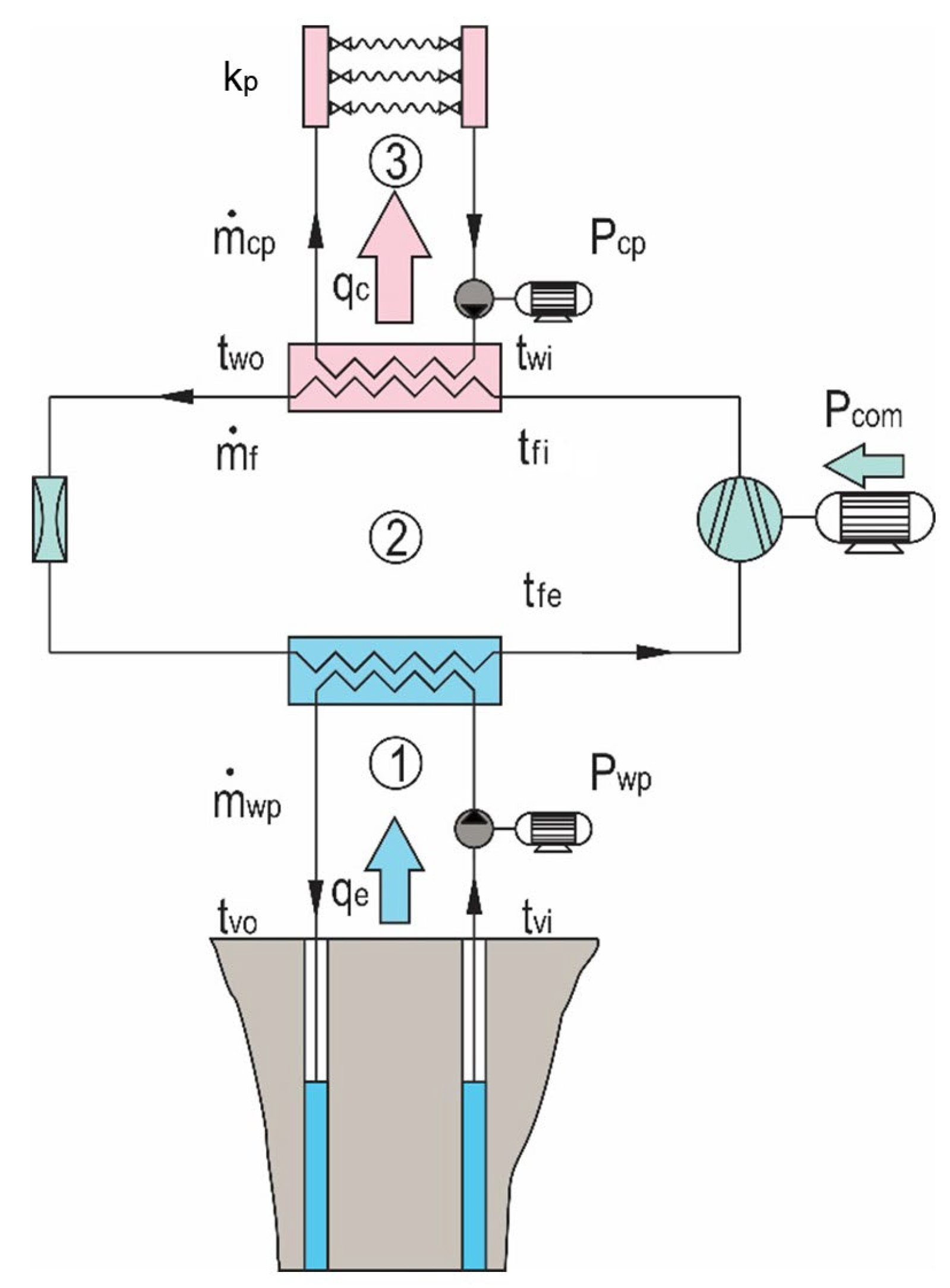
2. Physical System

Configuration of the physical system depends on the type of heat pump Figure 1. There are various heat pump heating systems used in practice [2,3,4,5,6,7,8,9,10]. However, the most energy-efficient water-to-water heat pump heating system is probably also the most commonly used one [11,14,15,16]. The statement is especially valid for the Pannonian Plain (Hungary, Serbia, Croatia), since in-ground drilling for a U-tube heat exchanger is relatively easy. Recently, air-to-air or air-o-water heat pumps have become more and more popular [2,3,4,5,6,7,8,9,10]. While their energy efficiency is lower, the price of the complete system is lower as well.

From the energetic and structural point of view, the water-to-water heat pump heating system consists of three heat carrier circuits, two water loops, and one refrigerant cycle. During operation, the working medium in all three loops flows and transports the heat from a lower temperature to a higher one. The energy for the flow is provided by electric motors.

3. Mathematical Methods

3.1. Description of the Method

The goal of energy optimization is to achieve the maximum $COP$. An analytical-numerical method was used for optimization. The objective functions are $CO{P}_c$ and $CO{P}_e$. The conditions for maximum $COP$ are the first derivatives of the $COP$ have to be equal to zero. The derivation was carried out indirectly, first according to power and then according to the mass flow rates [15,16]. Namely, the term functions in the $COP$ do not directly depend on the power, but on the mass flows. The functions are the heat flows ($q_1,$ $q_2$) in the condenser and the evaporator, the power of the pumps ($P_{cp}$, $P_{wp}$) and the efficiency of the pumps (${\eta }_{cp}$, ${\eta }_{wp}$). In the optimizer model, these functions were partially derived. The obtained derivatives were used in the equation of the maximum $COP$ condition.

In the optimizer model, the equations are algebraic, non-linear, coupled, and large. The equation system can be solved numerically.

3.2. Objective Functions of the Heating System—$COP$

$CO{P}_c$ applies to the condenser loop and it is suitable for determining the optimal power of the circulation pump, since some terms of $CO{P}_c$ are a function of the mass flow of hot water.

$$CO{P}_c=\frac{q_c\left({\stackrel{·}{m}}_{cp}\right)+P_{cp,e }\left({\stackrel{·}{m}}_{cp}\right)}{ P_{com,r }+P_{wp,r}+P_{cp,e }\left({\stackrel{·}{m}}_{cp}\right)·{{\eta }_{cp}}^{-1}\left({\stackrel{·}{m}}_{cp}\right)}$$

(1)

$CO{P}_e$ applies to the evaporator loop and is suitable for determining the optimum power of the well pump, since some terms in the $CO{P}_e$ are the function of the cold-water mass flow rate.

$$CO{P}_e=\frac{q_e\left({\stackrel{·}{m}}_{wp}\right)+P_{com,r}·{\eta }_{com}+P_{cp,e}}{P_{com,r}+P_{wp,e}\left({\stackrel{·}{m}}_{wp}\right)·{{\eta }_{wp}}^{-1}\left({\stackrel{·}{m}}_{wp}\right)+P_{cp,e}·{{\eta }_{cp}}^{-1}}$$

(2)

3.3. Local Energy Optimum as a Function of the Circulation Pump Power

In the equation of $CO{P}_c$, the terms of the heat flow in the condenser, the circulation pump power, and its efficiency are given as a function of the warm water mass flow rate.

Mathematically, the condition of the local energy optimum is the partial derivative of the $CO{P}_c$ with respect to the effective power of the circulation pump and the warm water mass flow rate. Based on the analytical extremum condition, the derivative should be equal to zero.

$$\frac{\partial CO{P}_c}{\partial {\stackrel{·}{m}}_{cp}}=\frac{\partial }{\partial {\stackrel{·}{m}}_{cp}}\left(\frac{q_c\left({\stackrel{·}{m}}_{cp}\right)+P_{cp,e}\left({\stackrel{·}{m}}_{cp}\right)}{P_{com,r}+P_{wp,r}+P_{cp,e}\left({\stackrel{·}{m}}_{cp}\right)·{{\eta }_{cp}}^{-1}\left({\stackrel{·}{m}}_{cp}\right)}\right)·\frac{\partial {\stackrel{·}{m}}_{cp}}{\partial P_{cp,e}}=0$$

(3)

The equation of the local energy optimum condition after the derivation is given below:

If: $P_{com,r}$ = var. const., $P_{wp,r}$ = var. const.,

$$\left(\frac{\partial q_c}{\partial {\stackrel{·}{m}}_{cp}{}_{}}·\frac{\partial {\stackrel{·}{m}}_{cp}}{\partial P_{cp,e}}+1\right)·\left(P_{com,r}+P_{wp,r}+\frac{P_{cp,e}}{{\eta }_{cp}}\right)-\left(q_c+P_{cp,e}\right)·\left({{\eta }_{cp}}^{-1}-\frac{P_{cp,e}}{{\eta }_{cp}{}^2}·\frac{\partial {\eta }_{cp}}{\partial {\stackrel{·}{m}}_{cp}{}_{}}·\frac{\partial {\stackrel{·}{m}}_{cp}{}_{}}{\partial P_{cp,e}}\right)=0$$

(4)

3.4. Local Energy Optimum as a Function of the Well Pump Power

In this case, the expression of $CO{P}_e$ contains the functions of the heat flow in the evaporator, the compressor real power and its efficiency are given as a function of the cold-water mass flow rate.

The condition of the local energy optimum, if the partial derivative of the $CO{P}_e$ with respect to the cold-water mass flow rate and the power of the well pump equals zero, is seen here.

$$\frac{\partial CO{P}_e}{\partial {\stackrel{·}{m}}_{wp}}\frac{\partial {\stackrel{·}{m}}_{wp}}{\partial P_{wp,e}}\frac{\partial }{\partial {\stackrel{·}{m}}_{wp}}\left(\frac{q_e\left({\stackrel{·}{m}}_{wp}\right)+P_{com,\mathrm{r}}·{\eta }_{com}+P_{cp,e}}{P_{com,r}+P_{wp,e}\left({\stackrel{·}{m}}_{wp}\right)·{{\eta }_{wp}}^{-1}\left({\stackrel{·}{m}}_{wp}\right)+P_{cp,e}·{{\eta }_{cp}}^{-1}}\right)·\frac{\partial {\stackrel{·}{m}}_{wp}}{\partial P_{wp,e}}=0$$

(5)

3.5. The Local Energy Optimum Condition after the Derivation Is as Follows

If: $P_{com,r}$ = var. const., $P_{wp,r}$ = var. const.,

$$\left(\frac{\partial q_e}{\partial {\stackrel{·}{m}}_{wp}}·\frac{\partial {\stackrel{·}{m}}_{wp}}{\partial P_{wp,e}}\right)·\left(P_{com,r}+\frac{P_{wp,e}}{{\eta }_{wp}}+\frac{P_{cp,e}}{{\eta }_{cp}}\right)-\left(q_e+P_{com,\mathrm{r}}+P_{cp,e}\right)·\left({{\eta }_{wp}}^{-1}-\frac{P_{wp,e}}{{\eta }_{wp}{}^2}·\frac{\partial {\eta }_{wp}}{\partial {\stackrel{·}{m}}_{wp}}·\frac{\partial {\stackrel{·}{m}}_{wp}}{\partial P_{wp,e}}\right)=0$$

(6)

3.6. The Global Multi Objective Energy Optimum

The equation system of the global multi objective energy optimum condition of the heat pump heating system involves the two local energy optimum condition Equations (4) and (6). The condition Equation (4) is as a function of the effective power of the circulation and (6) depends on the well pump effective power.

From a practical point of view, the global multi objective energy optimum is crucial because it incorporates both local energy optimums, the optimal mass flow rates of warm and cold water; therefore, the optimum power of the circulation and the well pumps can be determined as well [16].

4. Case Study

Energy optimization is a wide-ranging topic; therefore, in the case study, only the analytical-numerical energy optimization procedure is presented for determining the optimum power of the circulation pump in the warm water loop is to reveal the influence of the circulation pump power on the $COP$.

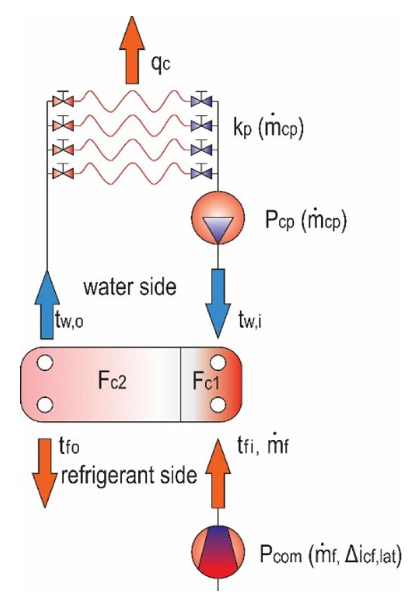
4.1. Physical Model of the Warm Water Loop

The active energy components of the warm water loop are the condenser, the compressor, the circulation pump, and the piping with the heating elements. In this case, the well pump is a passive participant, a variable constant.

In the plate heat exchanger, the high-temperature vapor flowing from the compressor transfers its heat to the warm water, thereby it is condensing. The warm water flows using the energy obtained from the circulation pump and transports the heat to the heating elements Figure 2.

1. Vaper cooling section, 2. vaper condensing section.

4.2. Basic Mathematical Model of the Condenser

Based on its operation, the condenser consists of the vapor cooling and condensation section, thus the basic model of the condenser is divided into two parts and involves three + three heat flows governing and several auxiliary equations [16].

4.2.1. Governing Equations of the Condenser

In the vapor cooling section, the three heat flow equations are:

Heat capacity decrement of the refrigerant is (Appendix A):

$$q_{c1}={\stackrel{·}{m}}_f·\Delta i_{f1}\cong {\stackrel{·}{m}}_f·C_{pf}·\left(t_{fi}-t_{fm}\right), C_{pf}=average$$

(7)

Heat transfer over the wall is:

$$q_{c1}=k_1·F_{c1}·\Delta t_{ln1}$$

(8)

Heat capacity increment of the water is:

$$q_{c1}={\stackrel{·}{m}}_{cp}·\Delta i_w\cong {\stackrel{·}{m}}_{cp}·C_{pw}·\left(t_{wm}-t_{wi}\right) C_{pw}\cong const.$$

(9)

In the condensation section, the three heat flow equations are:

Latent heat of the refrigerant is:

$$q_{c2}={\stackrel{·}{m}}_f·\Delta i_{f,lat}\cong {\stackrel{·}{m}}_f·\left(a_{c0}+a_{c1}·t_{cfo}^1+a_{c2}·t_{cfo}^2+\cdots \right), {\mathrm{t}}_{\mathrm{fm}}={\mathrm{t}}_{\mathrm{fo}}\cong \mathrm{const}.$$

(10)

Heat transfers over the wall is:

$$q_{c2}=k_2·F_{c2}·\Delta t_{ln2}$$

(11)

Heat capacity increment of the water is:

$$q_{c2}={\stackrel{·}{m}}_{cp}·\Delta i_{w2}\cong {\stackrel{·}{m}}_{cp}·C_{pw}·\left(t_{wo}-t_{wm}\right)$$

(12)

The total heat transfer surface of the condenser is:

$$F_c=F_{c1}+F_{c2}$$

(13)

The total heat flow in the condenser is:

$$q_c=q_{c1}+q_{c2}$$

(14)

4.2.2. Auxiliary Equations

The logarithmic temperature difference in the vapor cooling and condensation section was approximated to the arithmetic. This linearization requires the analytical optimization procedure. The formed deviation between the logarithmic and arithmetic temperature difference is only 0.2% [16].

The logarithmic and arithmetic temperature difference of the vapor cooling section:

$$\Delta t_{ln1}=\left(\left(t_{fi}-t_{wi}\right)-\left(t_{fm}-t_{vm}\right)\right)·{\left(ln\frac{t_{fi}-t_{wi}}{t_{fm}-t_{wm}}\right)}^{-1}\cong \frac{\left(\left(t_{fi}-t_{wi}\right)+\left(t_{fm}-t_{wm}\right)\right)}{2}$$

(15)

The logarithmic and arithmetic temperature difference of the vapor condensing section:

$$\Delta t_{ln2}=\left(\left(t_{fm}-t_{wm}\right)-\left(t_{fo}-t_{wo}\right)\right)·{\left(\ln \frac{t_{fm}-t_{wm}}{t_{fo}-t_{wo}}\right)}^{-1}\cong \frac{\left(\left(t_{fm}-t_{wm}\right)+\left(t_{fo}-t_{wo}\right)\right)}{2}$$

(16)

The overall heat transfer coefficient is approximated, since the wall thickness of the heat exchanger is (0.3–0.5) mm, therefore the δ/λ ≅ 0 term in the equation is equal to or close to zero. The heat transfer coefficient of the water is the same in the cooling and condensation section.

The overall heat transfer coefficient [19,20] is:

$$k_{1,2}={\left(\frac{1}{{\alpha }_w}+\sum \frac{\delta }{\lambda }+\frac{1}{{\alpha }_{f1,2}}\right)}^{-1}\cong \frac{{\alpha }_w·{\alpha }_{f1,2}}{{\alpha }_w+{\alpha }_{f1,2}}$$

(17)

1. Vapor cooling section,

2. Condensation section.

4.3. Modified Mathematical Model of the Condenser

The basic model of the condenser is not applicable to the analytical optimization procedure, since contains six unknown variables. The modification eliminated the unknown temperatures and surfaces (${\mathrm{t}}_{\mathrm{fm}},{\mathrm{t}}_{\mathrm{vm}},{\mathrm{t}}_{\mathrm{fo}},{ \mathrm{t}}_{\mathrm{wo}},F_{c1}, F_{c2})$, while the known input data ($F_c,{ \mathrm{t}}_{\mathrm{wi}},{\mathrm{t}}_{\mathrm{fe}}, P_{wp,r},P_{com,r},$) and the two unknown heat flows ($q_1$, $q_2)$ remain. As a result, the condenser’s modified model contains only two coupled algebraic equations with two unknown variables ($q_1$, $q_2)$

The unknown surfaces ($F_{c1}, F_{c2})$ are expressed from the equation of the overall heat flow (8), (11), and substituted into the total surface Equation (13).

Upon eliminating the unknown surfaces ($F_{c1}, F_{c2}),$ the first equation of the modified model is [16]:

$$F_c=\left(\frac{q_{\mathrm{c}1}}{k_1·\Delta t_{ln1}}+\frac{q_{c2}}{k_2·\Delta t_{ln2}}\right)$$

(18)

The unknown temperatures ($t_{fo},t_{vm}, t_{wo})$ are in the logarithmic − arithmetic temperature difference, their elimination is possible by substitution. The unknown temperatures were expressed from the heat flow equations of the vapor cooling (7), (9), and condensation (12) section, then the logarithmic − arithmetic temperature difference functions were substituted.

In the condensation section, the condensation heat flow using the latent heat was determined. In the analytical optimization procedure, the polynomial form is the most suitable.

$$q_{c2}={\stackrel{·}{m}}_f·\Delta i_{f,lat}\cong {\stackrel{·}{m}}_f·\left(a_{c0}+a_{c1}·t_{cfo}^1+a_{c2}·t_{cfo}^2+\cdots \right) t_{fo}\cong const.$$

(19)

The key task is to determine the unknown condensation temperature, $t_{fo}$. It is feasible by applying the heat flow equation of the vapor cooling section (20) and the equation of the compressor effective power (22), respectively.

The heat flow equation of the vapor cooling section is:

$$q_{c1}\cong {\stackrel{·}{m}}_f·C_{pf,c}·\left({\mathit{t}}_{\mathit{f}\mathit{i}}-t_{fo}\right)$$

(20)

The vapor temperature ${\mathit{t}}_{\mathit{f}\mathit{i}}$ at the condenser inlet is:

$$\frac{q_{c1}}{{\stackrel{·}{m}}_f·C_{pf,c}}+t_{fo}\cong {\mathit{t}}_{\mathit{f}\mathit{i}}$$

(21)

The compressor effective power is:

$$P_{com,e}\cong {\stackrel{·}{m}}_f·C_{pf,com}·\left({\mathit{t}}_{\mathit{f}\mathit{i}}-t_{fe}\right)$$

(22)

The vapor temperature ${\mathit{t}}_{\mathit{f}\mathit{i}}$ at the compressor outlet is:

$${\mathit{t}}_{\mathit{f}\mathit{i}}\cong \frac{P_{com,e}}{{\stackrel{·}{m}}_f·C_{pf,com}}+t_{fe}$$

(23)

The vapor temperature ${\mathit{t}}_{\mathit{f}\mathit{i}}$ at the compressor outlet and the condenser inlet is the same. Merging Equations (21) and (23), the condensation temperature can be expressed as:

$$t_{fo}\cong \frac{P_{com,e}}{{\stackrel{·}{m}}_f·C_{pf,com}}-\frac{q_{c1}}{{\stackrel{·}{m}}_f·C_{pf,c}}+t_{fe}$$

(24)

The second equation of the condenser’s modified model following the substitution of the condensation temperature (24) is:

$$q_{c2}={\stackrel{·}{m}}_f·\left(\begin{array}{c}{a}_{co}+a_{c1}·\frac{P_{com,e}}{{\stackrel{·}{m}}_f·C_{pf,com}}-\frac{q_{c1}}{{\stackrel{·}{m}}_f·C_{pf,c}}+t_{fe}\\ +a_{c2}·{\left(\frac{P_{com,e}}{{\stackrel{·}{m}}_f·C_{pf,com}}-\frac{q_{c1}}{{\stackrel{·}{m}}_f·C_{pf,c}}+t_{fe}\right)}^2\end{array}\right)$$

(25)

4.4. Mathematical Model of the Circulation Pump

The basic steady state-lumped model of the effective power of the circulation pump is:

$$P_{cp,e}={\stackrel{·}{m}}_w·{\rho }_w{}^{-1}·{{\displaystyle \sum }}_1^n\Delta p_i \left({\stackrel{·}{m}}_{cp}\right)$$

(26)

The pressure drops in the pipeline are a function of the water mass flow rate, according to the Darcy–Welsbach equation, as seen here.

$$\begin{gathered} {{\displaystyle \sum }}_1^n\Delta p_i \left({\stackrel{·}{m}}_{cp}\right)=\left({{\displaystyle \sum }}_{i=1}^n{\xi }_i\left(Re, \epsilon \right)·\frac{l_i}{d_i}+{{\displaystyle \sum }}_{i=1}^n{\xi }_{i,lok}\left(goem\right)\right)·\frac{1}{2·A_d{}^2}·\frac{{\stackrel{·}{m}}_{cp}{}^2}{{\rho }_w}= \\ =\frac{k}{{\rho }_w}·{\stackrel{·}{m}}_{cp}{}^2 \end{gathered}$$

(27)

Upon substituting the pressure drop (27), the modified equation of the effective power is:

$$P_{cp,e}=\frac{k}{{\rho }_w}·{\rho }_w{}^{-1}·{\stackrel{·}{m}}_{cp}{}^3=k_p·{\stackrel{·}{m}}_{cp}{}^3$$

(28)

The coefficient of the characteristics of the pipeline is:

$$k_p=k·{\rho }_w{}^{-2}\cong variable constant$$

(29)

In fact, the k term depends on the mass flow rate, since it exists in the Reynolds number, but its dependency is very weak, as confirmed by the measurement results, therefore it can be considered as a variable constant. The value of the k term is defined by the constructive shape and dimensions of the pipeline, and it is different for each case.

For the determination of real power, the dissipation of the power should be taken into account by using the efficiency [17].

$$P_{cp,r}=P_{cp,e}·{\eta }_{cp}{}^{-1}\left({\stackrel{·}{m}}_{cp}\right)$$

(30)

In this case, the efficiency factor [17] determination was performed based on the measured values of the real pump. Using the measured real and calculated effective pump power values, the efficiency was calculated and the ${\eta }_{cp}-P_{cp,e}$ polynomial was created [21].

$${\eta }_{cp}\left({\stackrel{·}{m}}_{cp}\right)=a_o+a_1·P_{cp,e}+a_2·P_{cp,e}{}^2+\cdots =a_o+a_1·k_p·{\stackrel{·}{m}}_{cp}{}^3+a_2·{\left(k_{cp}·{\stackrel{·}{m}}_{cp}{}^3\right)}^2$$

(31)

4.5. Mathematical Model of the Compressor

To determine the local optimum power of the circulating pump, the real power of the compressor is a known value and a variable constant. By applying the known real power, the effective power of the compressor is:

$$P_{com,e}=P_{com,r}·{\eta }_{com}\left(P_{com,r}\right)$$

(32)

In this case, the efficiency of the compressor was calculated using the measured real and calculated effective power values. The generated polynomial is [21]:

$${\eta }_{com}\left(P_{com,r}\right)=a_o+a_1·P_{com,r}+a_2·P_{com,r}{}^2+\cdots$$

(33)

The effective power can be used to determine the mass flow rate of the refrigerant and the vapor temperature on the compressor output.

The mass flow rate of the refrigerant is:

$${\stackrel{·}{m}}_f=P_{com,e}·{\left(i_{f,i}-i_{f,e}\right)}^{-1}$$

(34)

The vapor temperature at the compressor output is determined by applying the increment of the vapor enthalpy [22] by the compression, and the compressor effective power.

$$P_{com,e}={\stackrel{·}{m}}_f·\left(i_{f,i}-i_{f,e}\right)\cong {\stackrel{·}{m}}_f·C_{p,f,com}·\left(t_{f,i}-t_{f,e}\right)$$

(35)

The average specific heat of the vaper during compression is:

$$C_{p,f,com}=0.5·\left(C_{p,f}\left(t_{f,i}\right)+C_{p,f}·\left(t_{f,e}\right)\right)$$

(36)

The vapor temperature at the compressor output is:

$$t_{fi}\cong \frac{P_{com,e}}{{\stackrel{·}{m}}_f·C_{p,f,com}}+t_{fe}$$

(37)

4.6. Optimizer Model of the Warm Water Loop

In the optimizer model, the partial derivatives ($\frac{\partial q_{c1}+\partial q_{c2}}{\partial {\stackrel{·}{m}}_{cp}},\frac{\partial {\stackrel{·}{m}}_{cp}}{\partial P_{cp,e}},\frac{\partial {\eta }_{cp}}{\partial {\stackrel{·}{m}}_{cp}}$) of the energy optimum condition of Equation (4) should be determined.

4.6.1. Heat Flow Derivatives of the Condenser

The partial derivative of the first modified equation of the condenser, with respect to the mass flow rate of warm water is:

$$\frac{\partial F_c}{\partial {\stackrel{·}{m}}_{cp}}=\frac{\partial }{\partial {\stackrel{·}{m}}_{cp}}\left(\frac{q_{c1}}{k_{c1}·\Delta t_{c,ln1}}+\frac{q_{c2}}{k_{c2}·\Delta t_{c,ln2}}\right)=0 F_c=\mathrm{var}.\mathrm{const}.$$

(38)

Following derivation:

$$\begin{gathered} \frac{\frac{\partial q_{c1}}{\partial {\stackrel{·}{m}}_{cp}}·\left(k_{c1}·\Delta t_{c,ln1}\right)-q_{c1}·\left(\frac{\partial k_{c1}}{\partial {\stackrel{·}{m}}_{cp}}·\Delta t_{c,ln1}+k_{c1}·\frac{\partial ·t_{c,ln1}}{\partial {\stackrel{·}{m}}_{cp}}\right)}{{\left(k_{c1}·\Delta t_{c,ln1}\right)}^2}+ \\ +\frac{\frac{\partial q_{c2}}{\partial {\stackrel{·}{m}}_{cp}}·\left(k_{c2}·\Delta t_{c,ln2}\right)-q_{c2}·\left(\frac{\partial k_{c2}}{\partial {\stackrel{·}{m}}_{cp}}·\Delta t_{c,ln2}+k_{c2}·\frac{\partial ·t_{c,ln2}}{\partial {\stackrel{·}{m}}_{cp}}\right)}{{\left(k_{c2}·\Delta t_{c,ln2}\right)}^2}=0 \end{gathered}$$

(39)

The partial derivative of the second modified equation of the condenser, with respect to the mass flow rate of warm water is:

$$\frac{\partial q_{c2}}{\partial {\stackrel{·}{m}}_{cp}}=\frac{\partial }{\partial {\stackrel{·}{m}}_{cp}}\left({\stackrel{·}{m}}_f·\left(\begin{array}{c}{a}_{co}+a_{c1}·\frac{P_{com,e}}{{\stackrel{·}{m}}_f·C_{pf,com}}-\frac{q_{c1}}{{\stackrel{·}{m}}_f·C_{pf,c}}+t_{fe}\\ +a_{c2}·{\left(\frac{P_{com,e}}{{\stackrel{·}{m}}_f·C_{pf,com}}-\frac{q_{c1}}{{\stackrel{·}{m}}_f·C_{pf,c}}+t_{fe}\right)}^2\end{array}\right)\right)$$

(40)

The mass flow rate of the refrigerant does not directly depend on the mass flow rate of the warm water.

$${\stackrel{·}{m}}_f\ne f\left({\stackrel{·}{m}}_{cp}\right) > \frac{\partial {\stackrel{·}{m}}_f}{\partial {\stackrel{·}{m}}_{cp}}=0$$

(41)

Following derivation, the final form is:

$$\frac{\partial q_{c2}}{\partial {\stackrel{·}{m}}_{cp}}=\left(a_{c1}+a_{c2}·\left(\frac{P_{com,e}}{{\stackrel{·}{m}}_f·C_{pf,com}}-\frac{q_{c1}}{{\stackrel{·}{m}}_f·C_{pf,c}}+t_{fe}\right)\right)\left(\frac{-1}{{\stackrel{·}{m}}_f·C{p}_{cfc}}·\frac{\partial q_{c1}}{\partial {\stackrel{·}{m}}_{cp}}\right)$$

(42)

4.6.2. Partial Derivative of the Circulation Pump Effective Power

The partial derivative of the effective power of the circulation pump, with respect to the mass flow rate of warm water is:

$$\frac{\partial P_{cp,e}}{\partial {\stackrel{·}{m}}_{cp}}=\frac{\partial \left(k_p·{\stackrel{·}{m}}_{cp}{}^3\right)}{\partial {\stackrel{·}{m}}_{cp}}=k_p·3·{\stackrel{·}{m}}_{cp}{}^2$$

(43)

From the above partial derivative:

$$\frac{\partial {\stackrel{·}{m}}_{cp}}{\partial P_{cp,e}}={\left(k_p·3·{\stackrel{·}{m}}_{cp}{}^2\right)}^{-1}$$

(44)

4.6.3. Partial Derivative of the Circulation Pump Efficiency

The partial derivative of efficiency as a function of the mass flow rate of warm water is:

$$\frac{\partial {\eta }_{cp}}{\partial {\stackrel{·}{m}}_{cp}}=\frac{\partial }{\partial {\stackrel{·}{m}}_{cp}}\left(a_o+a_1·k_p·{\stackrel{·}{m}}_{cp}{}^3+a_2·{\left(k_p·{\stackrel{·}{m}}_{cp}{}^3\right)}^2\right)$$

(45)

Following derivation:

$$\frac{\partial {\eta }_{cp}}{\partial {\stackrel{·}{m}}_{cp}}=a_1·k_p·3·{\stackrel{·}{m}}_{cp}{}^2+a_2·k_p{}^2·6·{\stackrel{·}{m}}_{cp}{}^5$$

(46)

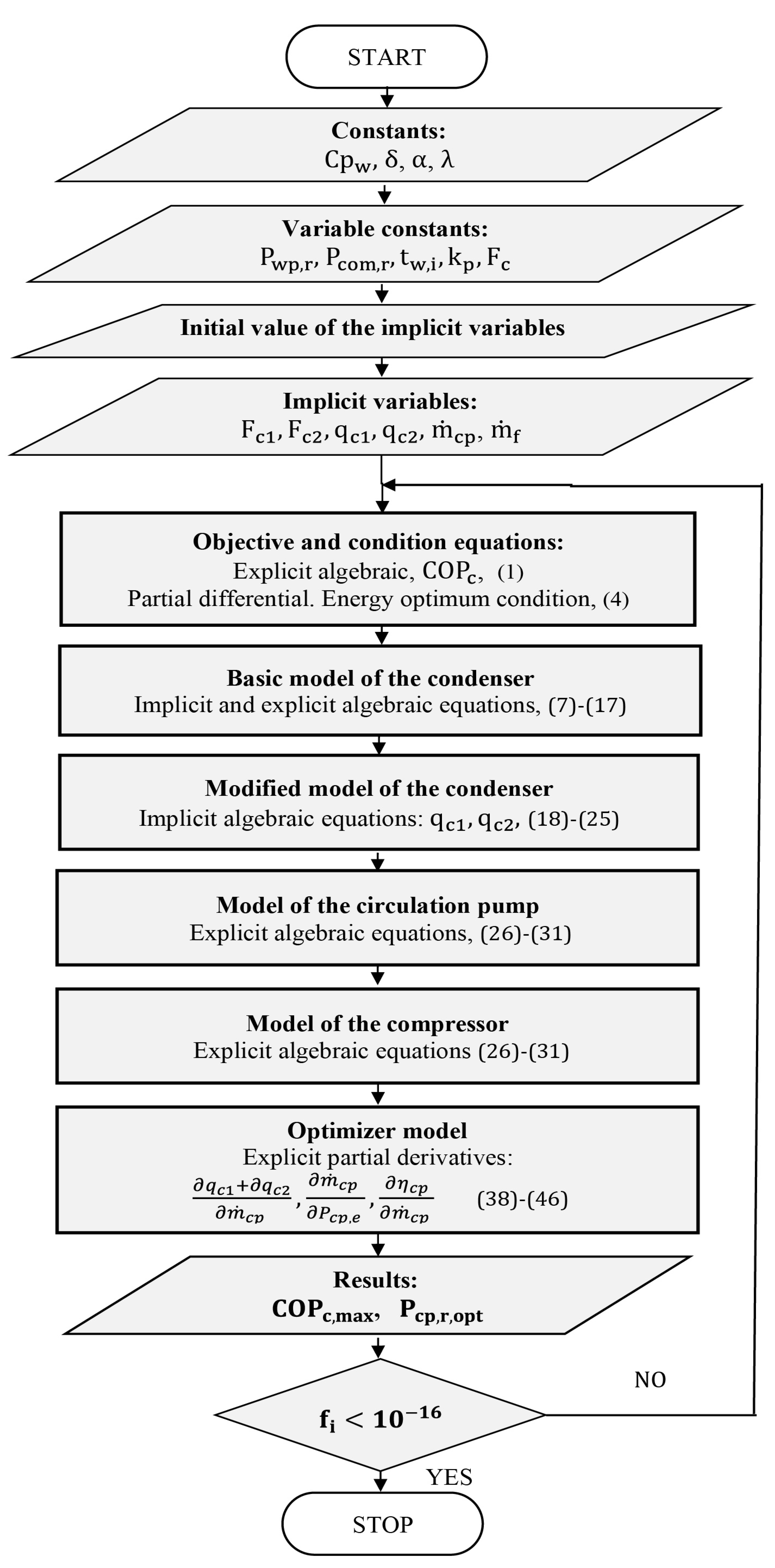
5. Numerical Procedure

In the optimizer model after partial derivation the obtained equation system is composed of the coupled, nonlinear, algebraic and large equations. Such an equation system can be solved numerically, e.g., by applying the Newton linearization and Gauss elimination method [18]. The method is iterative, most of the algebraic equations are implicit, therefore the value of the unknown variables at the start should be assumed. The experience shows that the assumed values should be close to the solution, otherwise the iterations do not converge Figure 3.

The Maximum $CO{P}_c$ of the Heat Pump Heating System

The solution of the algebraic equation system of the optimizer model gives the optimum value of the warm water mass flow rate. Based on this, the optimum power and efficiency of the circulation pump can be calculated. The procedure also determines the heat flow of the vapor cooler and the condensation section, as well as the local optimum $CO{P}_{c,max}$ [18].

6. Measurements and Measuring System

The accuracy of the analytical-numerical energy optimization procedure was validated by measurements. The input data for the optimization procedure and the measurements are the same.

Inputs of the series of measurements, Table 1:

• Refrigerant vapor temperature at the input of the compressor $t_e=4 \left[°\mathrm{C}\right]$,
• Warm water temperature at the input of the condenser $t_{w,i}=40 \left[°\mathrm{C}\right]$,
• Series of adjusted pressure heads of the circulation pump $\Delta p_{cp}=2, 4, 6, 8, 10, 12 \left[\mathrm{m}\right]$,
• The real powers of c. pump $P_{cp,\mathrm{r}}=44, 91, 152, 222, 298, 379 \left[\mathrm{W}\right]$,
• Well pump real power $P_{wp,\mathrm{r}}=505 \left[\mathrm{W}\right]$.

Table 1. Data of the series of measurements.

$t_{w,o} \left[°\mathrm{C}\right]$	47.3	45.2	44.2	43.7	43	42.85
$t_{w,i}$ $\left[°\mathrm{C}\right]$	40	40	40	40	40	40
${\stackrel{·}{m}}_{cp} \left[\raisebox{1ex}{$\mathrm{kg}$}\!\left/ \!\raisebox{-1ex}{$\mathrm{s}$}\right.\right]$	0.455	0.657	0.826	0.947	1.168	1.21
$q_c{}^{*} \left[\mathrm{W}\right]$	13,889	14,302	14,526	14,673	14,587	14,678
$\Delta {\mathit{p}}_{\mathit{c}\mathit{p}} \left[m\right]$	2	4	6	8	10	12
$\Delta p_{cp} \left[\raisebox{1ex}{$\mathrm{N}$}\!\left/ \!\raisebox{-1ex}{${\mathrm{m}}^2$}\right.\right]$	19,620	39,240	58,860	78,480	98,100	117,720
${\mathit{P}}_{\mathit{c}\mathit{p},r} \left[W\right]$	44	91	152	222	298	379
$P_{cp,\mathrm{e}} \left[\mathrm{W}\right]$	8.93	25.78	48.6	74.32	107.13	142.44
${\eta }_{cp} \left[-\right]$	0.203	0.283	0.326	0.334	0.359	0.376
$P_{com,\mathrm{r}} \left[\mathrm{W}\right]$	4192	4128	4116	4044	4028	3984
${\eta }_{com} \left[-\right]$	0.83	0.84	0.85	0.865	0.867	0.87
$P_{wp,\mathrm{r}} \left[\mathrm{W}\right]$	505	505	505	505	505	505
$\mathit{C}\mathit{O}{\mathit{P}}_{\mathit{c}} \left[-\right]$	2.939	3.010	3.035	3.059	3.066	3.019

Table 1. Data of the series of measurements.

$t_{w,o} \left[°\mathrm{C}\right]$	47.3	45.2	44.2	43.7	43	42.85
$t_{w,i}$ $\left[°\mathrm{C}\right]$	40	40	40	40	40	40
${\stackrel{·}{m}}_{cp} \left[\raisebox{1ex}{$\mathrm{kg}$}\!\left/ \!\raisebox{-1ex}{$\mathrm{s}$}\right.\right]$	0.455	0.657	0.826	0.947	1.168	1.21
$q_c{}^{*} \left[\mathrm{W}\right]$	13,889	14,302	14,526	14,673	14,587	14,678
$\Delta {\mathit{p}}_{\mathit{c}\mathit{p}} \left[m\right]$	2	4	6	8	10	12
$\Delta p_{cp} \left[\raisebox{1ex}{$\mathrm{N}$}\!\left/ \!\raisebox{-1ex}{${\mathrm{m}}^2$}\right.\right]$	19,620	39,240	58,860	78,480	98,100	117,720
${\mathit{P}}_{\mathit{c}\mathit{p},r} \left[W\right]$	44	91	152	222	298	379
$P_{cp,\mathrm{e}} \left[\mathrm{W}\right]$	8.93	25.78	48.6	74.32	107.13	142.44
${\eta }_{cp} \left[-\right]$	0.203	0.283	0.326	0.334	0.359	0.376
$P_{com,\mathrm{r}} \left[\mathrm{W}\right]$	4192	4128	4116	4044	4028	3984
${\eta }_{com} \left[-\right]$	0.83	0.84	0.85	0.865	0.867	0.87
$P_{wp,\mathrm{r}} \left[\mathrm{W}\right]$	505	505	505	505	505	505
$\mathit{C}\mathit{O}{\mathit{P}}_{\mathit{c}} \left[-\right]$	2.939	3.010	3.035	3.059	3.066	3.019

In order to calculate the total heat flow, the water caloric equation was applied, since the inlet and outlet water temperatures and mass flow rate are measured.

$$q_c{}^{*}=C_{pw}·{\stackrel{·}{m}}_{cp}·\left(t_{w,o}-t_{w,i}\right)$$

(47)

6.1. Measuring System

The measuring instruments of the measuring system include the following:

• Glass-tube alcohol thermometers, 0.1 °C accuracy, range 0–100 °C,
• Insa type water volumetric flow meter with a ±2% accuracy, range 0–100 m³,
• Refco type manometers with a ±2% accuracy, range 0–30 bar for measuring the different pressure produced by the circulation pump,
• Voltage and ampere meter for measuring the power of the compressor and well pump, ±1% accuracy, range 0–600 V, 0–20 A,
• Stopwatch to determine the water volumetric flow rate, digital.

6.2. Physical System

The components of the physical system upon which the measurements were performed, Figure 4:

• Heat pump (Tera Term, Co.) with a scroll compressor with a nominal power of 4000 W and plate heat exchangers with nominal 2 m², i.e., 1.6 m² effective surface,
• Circulation pump (Wilo, Dortmund, Germany) with a nominal power of 400 W and frequency-control that enables the control of differential pressure, power, and number of revolutions.

Figure 4. Photo of the measurement system with the heat pump.

Figure 4. Photo of the measurement system with the heat pump.

6.3. Measurement Process

The values of the five variables (${\stackrel{·}{m}}_{cp},{ \mathrm{t}}_{\mathrm{wi}},{\mathrm{t}}_{\mathrm{wo}}, P_{wp,r},P_{com,r},$) were simultaneously read in 40 °C water temperature at the inlet of the condenser. During the series of measurements, the water mass flow rate was constant and its value was determined indirectly. The volume of the flow water was measured by the water meter. The volume was divided by the time shown on the stopwatch and multiplied by the density of the water.

The circulation pump power was measured by the built-in electronic instrument of the pump and the current value was read from the display. The instantaneous value of the compressor power was calculated using the measured values of the current and voltage. The outlet and inlet water temperatures were read directly from the 0.1 [°C] alcohol thermometers.

Based on the measured values Table 1. the $CO{P}_c-P_{cp}$ diagram was constructed Figure 5. The simulated result obtained by the analytical-numerical optimization procedure presented in the Figure 6.

Comparison of the simulated and measured results

Table 2. Comparison of the results obtained by the analytical optimization or measurements.

	$\mathit{C}\mathit{O}{\mathit{P}}_{\mathit{c},\mathit{m}\mathit{a}\mathit{x} }\left[-\right]$	${\mathit{P}}_{\mathit{c}\mathit{p},\mathit{o}\mathit{p}\mathit{t}} \left[\mathbf{W}\right]$
Analytical optimization	3.096	238.5
Measurements	3.077	242
Difference	0.019/3.077 = 0.006 0.6%	3.5/238.5 = 0.015 1.5%

.

7. Results and Discussion

The heating system has nine degrees of freedom, but only three are important from the point of view of energy optimization. Separately, two local energy optimums and these two locals together form the global multi energy optimum. To determine the optimums, we used an analytical-numerical procedure. The advantage of the analytical method is that it creates a connection between mathematics and physics. The disadvantage is that it requires a higher level of mathematical knowledge.

The objective functions are the $CO{P}_c$ and $CO{P}_e$ values of the system, expanded with mass flow rates and efficiencies of pumps and a compressor, therefore, they follow reality approximately well, and can be they considered almost real.

The aim of the optimization is to determine the optimal power of the two pumps; therefore, $CO{P}_c$ refers to the warm water loop with the condenser, while $CO{P}_e$ refers to the cold-water loop with the evaporator.

Since the heat flows, powers, and efficiencies in the $COP$ are functions of the mass flow rates, the partial differentiation of the $COP$ was carried out indirectly when determining the optimum conditions. First according to the powers, then according to the mass flow rates.

Nowadays, the majority of the water-to-water heat pump heating systems operate with on-off control, so the mathematical description of the system elements is possible with stationary and lumped equations. Such a system of equations enables the application of an analytical optimization procedure. The model of the system had to be designed according to the expectations of the analytical procedure. The six equations in the basic condenser model contain six unknown and several known variables. The unknowns were eliminated by merging the equations. The modified model contains only two equations and two unknown variables, i.e., two heat flows.

A key problem was the determination of the condensation temperature using the known variables. As a solution, the vapor temperatures leaving the compressor and entering the condenser were equalized. The Equations used are (20)–(23), and the result is (24).

The results obtained by the analytical-numerical procedure were validated by the measurements. The measurements were carried out with traditional instruments. The reliability of the measurement depended on the accuracy of the instruments and the person reading the values.

The important recognition that the optimization of the circulation pump power increases the $CO{P}_c$ value to a small extent. It was one of the reasons why, in the case study, the optimal power of the circulation pump was determined separately.

The $CO{P}_c-P_{cp}$ diagram in Figure 5 was constructed based on the measured values presented in Table 1. From this diagram, the maximum $CO{P}_{c,max}$ and the real optimum power $P_{cp,r}$ of the circulation pump can be visually determined. The diagram was created using a program that provides an exact numerical calculation of the $CO{P}_{c,max}$ and $P_{cp,r}$ as well. Both the calculations and the diagram indicate that the heating system has a local maximum at $CO{P}_{c,max }=3.077$ when the real optimum power of the circulation pump is $P_{cp,r}=242 \left[\mathrm{W}\right]$. At the same time, the values of the real power of the compressor and the well pump are constant: $P_{com,r}=4050 \left[\mathrm{W}\right]$, $P_{wp,r}=505 \left[\mathrm{W}\right]$.

Table 2 highlights that the results of the comparisons that prove the accuracy of the optimization procedure. Since the value of the $CO{P}_{c,max}$ is 0.6%, the optimum power of the circulation pump $P_{cp,opt}$ is 1.5% different, which is obtained with the optimization and the measurements.

In order to achieve the energy optimum in each operating point, the condition is that in this point, the power of the circulation pump should be optimal. Based on the control function, a control algorithm can be created. The controller measures the inlet water temperature and based on that, it calculates the optimum power and optimum revolution of the pump. The revolution can be realized using a frequency converter [13].

8. Conclusions

• The analytical part of the energy optimization procedure provides a linked insight into the interaction between mathematics and the physical system. The numerical part of the procedure provides accurate results for the local and global multi objective optimum power of the pumps,
• The advantage of the procedure is, by varying the temperature of the input warm water, it is possible to determine the optimal power of the circulation pump and the maximum $CO{P}_{c,max}$ in each operation point,
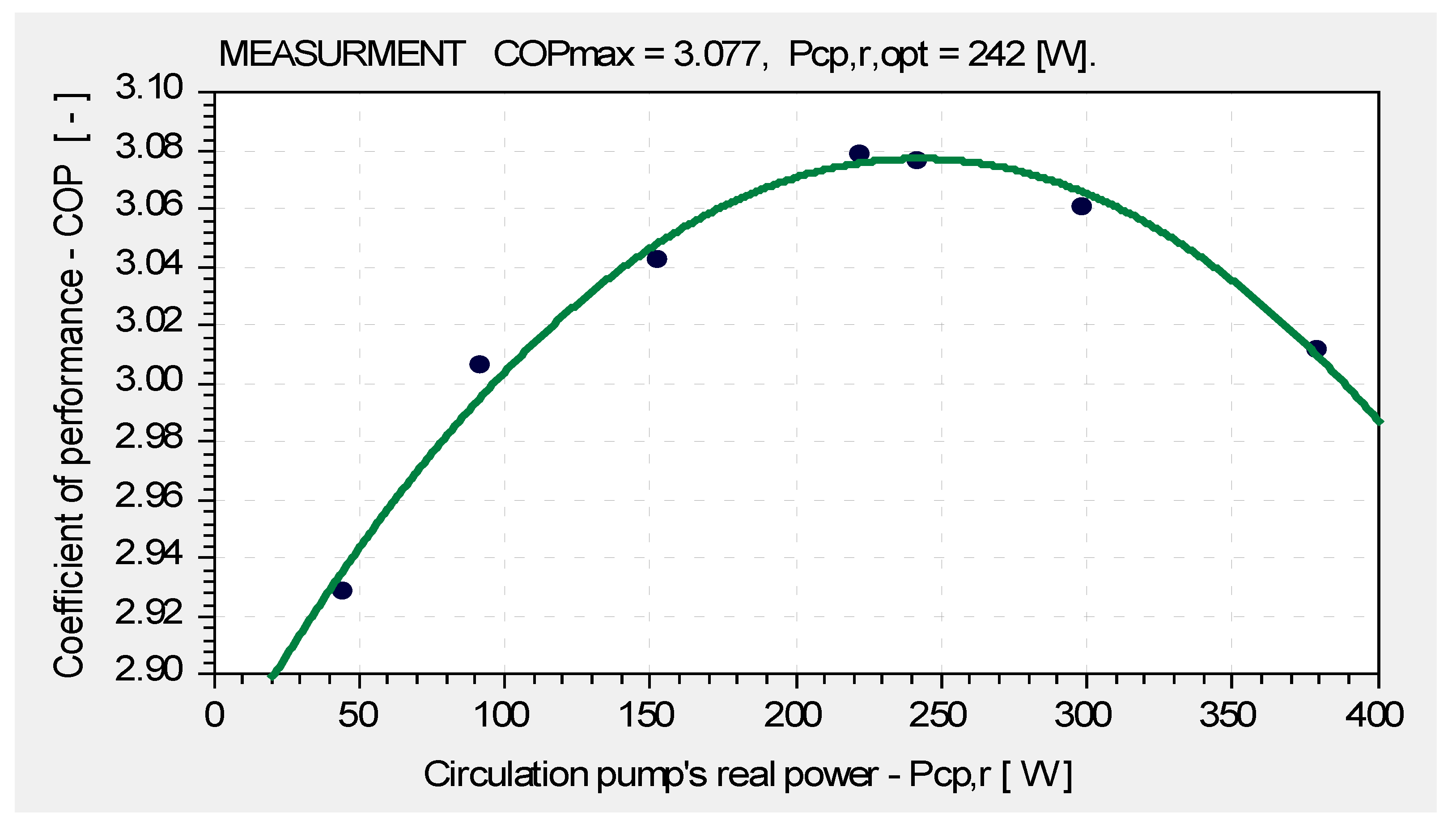
• The accuracy of the energy optimization procedure was proven through measurements. The difference in the maximum $CO{P}_{c,max}$ is 0.6% and 1.5% in the optimal power of the circulation pump, only. Table 2,
• The algorithm presents the complete mathematical method of the procedure with the type and number of variables,
• The values obtained by the procedure presented in tables and graphs provide an important guide for practice. The evaluation with numbers and data can be found in the points below,
• The efficiency of the circulation pump has a significant impact on the $CO{P}_{c,max}$, since its values are small, varying between 0.203 and 0.376 despite the fact that the real power is 242 [W] only,
• The compressor efficiency is significantly better and varies in the narrower range of 0.83–0.87 (measured), but its power is 4050 [W], so the influence of the compressor’s efficiency on the $CO{P}_c$ is also significant,
• The simulation value of the maximum $CO{P}_{c,max}$ without the efficiency of the compressor and circulation pump is $CO{P}_{c,max}=3.61$. With the efficiencies, based on the measurements, its value is only $CO{P}_{c,max}=3.07$ or the analytically-numerically optimized value is $CO{P}_{c,max}=3.091$ In percentages, the $CO{P}_{c,max}$ has $\left(17.3-16.8\right)\%$ times higher value, as calculated without efficiencies,
• The $CO{P}_c-P_{cp,r}$ parabolic graph (Figure 5) is smooth and flat, the $CO{P}_c$ difference is only $CO{P}_{c,max}-CO{P}_{c,min}=0.147$, so the effect of the power of the circulation pump on the $CO{P}_c$ is weak. Although, the increment of the real power of the circulation pump is relatively large 44 − 379 = 335 W, the rate of change is 379:44 = 8.6, (860%),
• Since the $CO{P}_c$ graph is flat, reducing the power of the pump only slightly reduces the $CO{P}_c$ value. So, a pump of 100 W that has less than the optimal power of 242 W, reduces the $CO{P}_c$ by only 1.2%. Therefore, it is reasonable to carry out the multi objective optimization using the economic and energy objectives,
• At the optimum point, the measured and optimized value of the circulation pump is 242 W and 238.5 W, while the compressor power is 4050 W. The power ratio is 4050:242 = 16.7. Therefore, the dominance of the compressor power on the $CO{P}_c$ is significantly larger, in proportion to the ratio of the powers,
• By optimizing the power of the circulation pump, the $CO{P}_c$ value increases approximately, $\Delta CO{P}_c=3.096-2.939=0.157$ i.e., $0.157:2.939=0.0534, 5.34\%$. However, by optimizing the power of the circulation and well pumps globally, the $CO{P}_c$ increase will be significantly greater.

References

- Jensen, B.J.; Skogestad, S. Degrees of freedom and optimality of sub-cooling. Comput. Chem. Eng. 2007, 31, 712–721. [Google Scholar] [CrossRef]
- Olympios, V.A.; Sapin, P.; Freeman, J.; Olkis, C.; Markides, N.C. Operational optimisation of an air-source heat pump system with thermal energy storage for domestic applications. Energy Convers. Manag. 2022, 273, 116426. [Google Scholar] [CrossRef]
- Ma, R.; Qiao, H.; Yu, X.; Yang, B.; Yang, H. Thermo-economic analysis and multi-objective optimization of a reversible heat pump-organic Rankine cycle power system for energy storage. Appl. Therm. Eng. 2022, 220, 119658. [Google Scholar] [CrossRef]
- Atasoy, E.; Çetin, B.; Bayer, O. Experiment-based optimization of an energy-efficient heat pump integrated water heater for household appliances. Energy 2022, 245, 123308. [Google Scholar] [CrossRef]
- Zhou, K.; Mao, J.; Li, Y.; Zhang, H. Performance assessment and techno-economic optimization of ground source heat pump for residential heating and cooling: A case study of Nanjing, China. Sustain. Energy Technol. Assess. 2020, 40, 100782. [Google Scholar] [CrossRef]
- Krützfeldt, H.; Vering, C.; Mehrfeld, P.; Müller, D. MILP design optimization of heat pump systems in German residential buildings. Energy Build. 2021, 249, 111204. [Google Scholar] [CrossRef]
- Hosseinnia, M.S.; Sorin, M. Techno-economic approach for optimum solar assisted ground source heat pump integration in buildings. Energy Convers. Manag. 2022, 267, 115947. [Google Scholar] [CrossRef]
- Delač, B.; Pavković, B.; Grozdek, M.; Bezić, L. Cost Optimal Renewable Electricity-Based HVAC System: Application of Air to Water or Water to Water Heat Pump. Energies 2022, 15, 1658. [Google Scholar] [CrossRef]
- Nordgård-Hansen, E.; Kishor, N.; Midttømme, K.; Risinggård, V.R.; Kocbach, J. Case study on optimal design and operation of detached house energy system: Solar, battery, and ground source heat pump. Appl. Energy 2022, 308, 118370. [Google Scholar] [CrossRef]
- Halilovic, S.; Böttcher, F.; Kramer, C.S.; Piggott, D.M.; Zosseder, K.; Hamacher, T. Well layout optimization for groundwater heat pump systems using the adjoint approach. Energy Convers. Manag. 2022, 268, 116033. [Google Scholar] [CrossRef]
- Santa, R.; Garbai, L.; Fürstner, I. Optimization of heat pump system. Energy 2015, 89, 45–54. [Google Scholar] [CrossRef]
- Granryd, E. Analytical expressions for optimum flow rates in evaporators and condensers of heat pumping systems. Int. J. Refrig. 2010, 33, 1211–1220. [Google Scholar] [CrossRef]
- Edwards, K.C.; Finn, D.P. Generalized water flow rate control strategy for optimal part load operation of ground source heat pump systems. Appl. Energy 2015, 150, 50–60. [Google Scholar] [CrossRef]
- Nyers, A. Víz-Víz Hőszivattyús Fűtési Rendszerek Energetikai Optimizálása. Ph.D. Thesis, Gépészmérnöki Kar, BMGE, Budapest, Hungary, 2016. Available online: https://repozitorium.omikk.bme.hu/bitstream/handle/10890/5352/tezis_hun.pdf?sequence=3&isAllowed=y (accessed on 3 March 2019).
- Nyers, J.; Nyers, A. Investigation of Heat Pump Condenser Performance in Heating Process of Buildings using a Steady-State Mathematical Model. Int. J. Energy Build. 2014, 75, 523–530. [Google Scholar] [CrossRef]
- Nyers, J. An analytical method for defining the pump’s power optimum of a water-to-water heat pump heating system using COP. Therm. Sci. 2017, 21, 1999–2010. [Google Scholar] [CrossRef]
- Eordoghne Miklos, M. Investigation of energy efficiency of pumping systems by a newly specified energy parameter. In Proceedings of the 11th International Symposium on Exploitation of Renewable Energy sources and Efficiency, EXPRES 2019, Subotica, Serbia, 11–13 April 2019; pp. 21–25, ISBN 978-86-919769-4-1. [Google Scholar]
- MATLAB Programming and Numeric Computing Platform. Available online: https://www.mathworks.com/products/matlab.html (accessed on 21 May 2020).
- Jokar, A.; Hosni, H.; Mohammad, J.; Eckels, S. Dimensional analysis on the evaporation and condensation of refrigerant R-134a in mini channel plate heat exchangers. Appl. Therm. Eng. 2006, 26, 2287–2300. [Google Scholar] [CrossRef]
- Ko, Y.M.; Jung, J.H.; Sohn, S.; Song, C.H.; Kang, Y.T. Condensation heat transfer performance and integrated correlations of low GWP refrigerants in plate heat exchangers. Int. J. Heat Mass Transf. 2021, 177, 121519. [Google Scholar] [CrossRef]
- Expert Curve Software Package. Available online: https://www.curveexpert.net/ (accessed on 25 September 2019).
- Astina, M.I.; Sato, H. A fundamental equation of state for 1,1,1,2-tetrafluoroethane with an intermolecular potential energy background and reliable ideal-gas properties. Fluid Phase Equilibria 2004, 221, 103–111. [Google Scholar] [CrossRef]