Abstract
In order to accurately calculate the geometric characteristics of the twin-screw compressor and obtain the optimal profile parameters, a calculation method for the geometric characteristics of twin-screw compressors was proposed to simplify the profile parameter design in this paper. In this method, the database of geometric characteristics is established by back-propagation (BP) neural network, and the genetic algorithm is used to find the optimal profile design parameters. The effects of training methods and hidden layers on the calculation accuracy of neural network are discussed. The effects of profile parameters, including inner radius of the male rotor, protection angle, radius of the elliptic arc, outer radius of the female rotor on the comprehensive evaluation value composed of length of the contact line, blow hole area and area utilization rate, are analyzed. The results show that the time consumed for the database established by BP neural network is 92.8% shorter than that of the traditional method and the error is within 1.5% of the traditional method. Based on the genetic algorithm, compared with the original profile, the blow hole area of the screw compressor profile optimized by genetic algorithm is reduced by 54.8%, the length of contact line is increased by 1.57% and the area utilization rate is increased by 0.32%. The CFD numerical model is used to verify the optimization method, and it can be observed that the leakage through the blow hole of the optimized model is reduced, which makes the average mass flow rate increase by 5.2%, indicating the effectiveness of the rotor profile parameter optimization method.
1. Introduction
With the development of industry and society, the problems of excessive energy consumption and environmental pollution have become increasingly prominent [1,2]. Relevant research shows that industrial energy consumption accounts for about 40% of electric energy consumption [3]. Therefore, reducing the energy consumption of industrial systems is of great significance for reducing energy consumption. As an industrial general machinery, improving the energy utilization rate of compressors is an important way to reduce energy consumption [4]. As the main component of gas compression, the twin-screw compressor is widely used in refrigeration, battery and other fields because of its simple structure, high reliability and exhaust pressure not limited by outlet pressure [5]. As the main parameter of twin-screw compressors, rotor geometric characteristics play an important role in the performance evaluation and optimization of twin-screw compressors [6].
In 1958, Frank Rosenblatt proposed the use of neural networks to identify and analyze the calculated database. Gan et al. [7] combines RBF neural network response surface and NSGA-II algorithm to propose a multi-objective optimization method for low noise design of multi-stage orifice plates. Wang et al. [8] used an artificial neural network for lithiumion battery temperature prediction which compared three neural network modeling techniques. Justin et al. [9] has used deep learning to develop partial differential equation (PDE) models in science and engineering.
In 1975, Professor Holland [10] from the University of Michigan first proposed the GA algorithm. He applied the principle of survival of the fittest in genetics to computational iteration and selected the best condition points by selection, crossover and mutation. Compared to particle swarm optimization and evolutionary algorithms, genetic algorithms have better global exploration capabilities, allowing all examples to move towards the optimal solution. Hernandez et al. [11] proposed an effective optimization design method composed of electromagnetic theory and intelligent algorithm, which can obviously promote the utilization efficiency and stability of YBCO coated conductors. Ahmed et al. [12] used an NSGA-II algorithm to optimize the design of GPU-3 Stirling engine. Wu [13] proposed a hybrid intelligent framework combining random forest and non-dominant classification NSGA-II to optimize shield construction parameters. Armin et al. [14] established an isothermal one-dimensional model of a fixed-bed reactor for oxidative dehydrogenation of propane over a V2O5/graphene catalyst, for which multi-objective optimization of propylene and COx yields was carried out. Erin et al. [15] examined the extent to which social disconnectedness and perceived isolation have distinct associations with physical and mental health among older adults. Ma et al. [16] selected three design variables related to the geometry of the blade and volute, such that the total head, efficiency and solid particle size of the pump were used as objective functions for parallel optimization. Sun et al. [17] used three different machine learning models to construct the approximate functional relationship between impeller solidity, stagger angle, skew and sweep parameters, and target values. However, no one has applied it to the screening of screw profiles. Li et al. [18] couples and clarifies NSGA III and SVM, and applies them to the whole machine MAP optimization. Researchers have also used other methods to optimize the profile parameters. Wu and Fong [19] used the SUMT (sequential unconstrained minimization technique) method to study parameters of the rotor profile optimization and non-undercut limits.
Due to the complexity of its structure, the characteristics of a screw compressor are not only affected by the basic laws of thermodynamics, but also by the production process and device structure, which makes it difficult to establish a high-precision simulation model [19]. Most of the simulation studies of twin-screw components focus on water injection lubrication [20], oil injection [21], rotor clearance [22], noise reduction [23], etc., and there are few detailed parametric analysis studies on the profiles.
For the twin-screw compressor, the traditional optimal profile parameter search calculation method is time-consuming and difficult to calculate. In this paper, a profile parameter optimization method was proposed, in which back-propagation (BP) neural network is used as data prediction and genetic algorithm as optimization. The purpose is to propose an accurate calculation method for the geometric characteristics of a twin-screw compressor, which makes the design of profile parameters more convenient. Firstly, the neural network model of geometric characteristics of a twin-screw compressor with the highest calculation accuracy is determined to predict the geometric characteristics of screw compressor quickly. Secondly, the comprehensive value of contact line length, leakage triangle size and area utilization coefficient are used as the evaluation index to find the optimal profile design parameters. Finally, the simulation software is used to compare the calculated parameters to verify the accuracy of the model.
2. Two-Screw Compressor Geometric Characteristics
2.1. Profile Parameters
Taking the Gute-Hoffnungs-Huette (GHH) modified profile as an example, after determining the line segment composition of the rotor profile and the number of rotor teeth, the geometric characteristics of the profile depend on several key parameters, including the pitch radius of the female rotor (R2), the inner radius of the male rotor (Ri), the outer radius of the female rotor (Ro), the protection angle (θ), the screw lead (τ), radius of the elliptic arc (a), etc., as shown in Figure 1a.
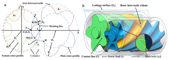
Figure 1.
Twin-screw rotor (a) End face diagram (b) Stereogram.
2.2. Calculation Method of Geometric Characteristics
The length of the contact line (L) refers to the spatial curve formed by the contact between the tooth surfaces of the two rotors when the rotor is engaged, as shown in the blue line segment in Figure 1b. The expression is:
In the formula, xi, yi, zi represents the curve parameter equation.
The blow hole area (Ab) refers to the triangular leakage channel between the top of the contact line and the cylinder when the vertex of the contact line fails to reach the intersection line of the cylinder holes of the male rotor and female rotor. It is represented by the yellow line segment in Figure 1b. The expression is:
In the formula, Zb represents the leakage surface, xi’, yi’ represents the derivative of the curve equation to the parameter, and ti and ti + 1 represent the starting point and end point parameters of the curve.
The area between teeth (A) refers to the gas area that can be accommodated by a single male rotor and female rotor tooth on the end surface, which is surrounded by multiple smooth curves and the head and tail of the tooth top arc, as shown in the orange area of the male rotor and female rotor in Figure 1a. The expression is:
Area utilization rate (Cn) refers to the utilization degree of the total area within the range of rotor diameter. The expression is:
In the formula, Z1 represents the number of teeth of the positive rotor, D1 represents the diameter of the positive rotor, and A1 and A2 represent the volume between the teeth of the positive rotor and the negative rotor, respectively.
2.3. Optimization Procedure
In this paper, the modified GHH profile is used as the optimization object, and the BP neural network is used to establish a rapid calculation data model of the geometric characteristics of the twin-screw compressor. The genetic algorithm is used to find the optimal design parameters under different operating conditions. The simulation model is used to verify the influence of the optimized profile on the rotor operation, and the effects of the profile parameters on the screw seal and volume characteristics are calculated and analyzed. In this process, the influence of the number of hidden layer neurons and the training function on the accuracy of geometric feature calculation is analyzed, and the influence of parameters such as population number and iteration number on the convergence of genetic algorithm is analyzed. In this paper, the BP neural network model and genetic algorithm model code written by MATLAB software are used to realize rapid calculation of geometric features and optimization of profile parameters, as shown in Figure 2.
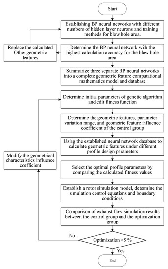
Figure 2.
The flow chart of genetic algorithm rotor optimization based on BP neural network.
3. Discrete Point Number Independence Verification
By comparing the profile results obtained under different discrete points and time steps with the profile results generated by SolidWorks software, the accuracy of the mathematical model calculation is verified. The tooth profile parameters of the control group are shown in Table 1.

Table 1.
Type line input parameters.
Profiles were generated with the discrete point numbers of 600, 1200, and 2400. Profile parameters and computation time were obtained and compared to choose the relatively optimal discrete point number, as shown in Table 2. As the number of point coordinates of the drawn profile increases, the calculated geometric feature error is smaller. However, when the number of point coordinates increases from 1200 to 2400 and from 2400 to 3600, the calculation time increases by two times but the calculation error decreases by 1.5% and 0.6%, respectively. Considering the influence of calculation time and calculation error, 2400 points are selected as calculation parameters.
Table 2.
Results of discrete point number independence verification.
4. BP Neural Network
In this paper, the BP neural network [24] is used to train the data set, including four input parameters: the inner radius of the male rotor (Ri) from 20 to 26 mm, the outer radius of the female rotor (Ro) from 0 to 2 mm, the protection angle (θ) from 0 to 10° and the radius of elliptic arc (a) from 8 to 12 mm; and three output parameters: blow hole area (Ab), length of the contact line (L) and area utilization rate (Cn).
The reliability of the trained neural network is verified by interpolation and extrapolation. Data interpolation can test the predictive ability of neural networks within the training range. Data extrapolation can reflect the predictive ability of neural networks outside the training range.
4.1. Parameter Definition of BP Neural Network
The total number of samples in the model is 2485. The 2236 samples were selected as the training sets. The 249 samples were randomly selected from the training samples as the interpolation set. The remaining 249 untrained samples were used as the extrapolation sets. Because the input packet array is small and the values of geometric features are relatively close, when only one mathematical model is established, the training effect is poor and the calculation is prone to large errors. Therefore, three separate BP neural networks are trained to predict blow hole area (Ab), length of the contact line (L) and area utilization rate (Cn) under different profile parameters.
Therefore, three separate BP neural networks are trained to predict blow hole area (Ab), length of the contact line (L) and area utilization rate (Cn) under different profile parameters. According to the empirical formula, the number of hidden layers is calculated as follows:
In the formula, M represents the number of input neurons, N represents the number of output neurons and H represents the number of hidden neurons.
In order to evaluate the accuracy of the calculated network, mean square error (MSE) and goodness-of-fitting index (R) are used as performance evaluation indicators. The calculation formula is:
In the formula, k represents the sample value, ki’ represents the average value of the sample and ki” represents the predicted sample value. n represents the number of samples.
4.2. Effects of Number of Hidden Neurons and Training Method on the Prediction Accuracy
Based on the Equation (5), the number of hidden neurons is determined to be eight to 18, and training is performed within this range to select the optimal number of nodes. For the training model, this paper considers three methods, the Levenberg–Marquardt method, the Bayesian regularization method and the Quantized conjugate gradient method. They use trainlm function, trainbr function and trainscg function as training functions, respectively. This is because the size of the problem type represented by the data is not clear before calculation. The trainscg function suitable for large problems, the trainlm function suitable for medium problems and the trainbr function suitable for small problems are selected, respectively. They have the advantages of high memory efficiency, fast calculation speed and wide application range, respectively. The calculation results are shown in Table 3.
Table 3.
Effects of training method and number of hidden neurons on calculation results.
In order to reduce the contingency of BP neural network calculation, each group of parameters was calculated 10 times. Five groups of data with the closest calculation results were selected from 10 groups of data. The average of these five sets of data is used as the calculation result.
It can be seen from Table 3 that for the neural network that calculate the blow hole area, the goodness-of-fitting index (R) increased, while the mean square error (MSE) decreased when the number of hidden neurons (H) increased. The Bayesian regularization method is more accurate than the other two methods. When H is 16, the model trained by the Bayesian regularization method has the highest calculation accuracy. For the neural network that calculate the length of contact line, the calculation accuracy is independent of H. The calculation accuracy of the three methods is similar. The Levenberg–Marquardt method has the highest calculation accuracy when H is 16, the Bayesian regularization method has the highest calculation accuracy when H is 16, and the quantitative conjugate gradient method has the highest calculation accuracy when H is 12. For the neural network that calculate the area utilization rate, the calculation accuracy is independent of H. Among them, the H is 16, while the model trained by Bayesian regularization method has the best calculation accuracy.
Three groups of models with the highest calculation accuracy were selected to establish a complete geometric feature BP neural network. Compared with the original calculation program, the calculation time is changed from 50 s to 3.6 s, which saves 92.8% of the time, and the calculation error is within 1.5%, which meets the accuracy requirements in engineering calculation.
5. Configuration Optimization
The four parameters of the inner radius of the male rotor (Ri), the outer radius of the female rotor (Ro), the protection angle (θ) and the radius of elliptic arc (a) are selected as optimization parameters. The fitness function is used as the evaluation criterion to find the optimal design parameters, and the effects of different population numbers, iteration times, crossover operators and mutation operators on the iterative convergence speed are analyzed. The fitness (F) function expression as the evaluation criterion is:
In the formula, IC, IL and IA represent the effects coefficient of area utilization rate, length of contact line and blow hole area, respectively. Cnt, Lt and Abt represent area utilization rate, length of contact line and blow hole area of treatment group, respectively. Abo, Cno and Lo represent area utilization rate, length of contact line and blow hole area of optimization group, respectively.
The GHH correction profile of five–six teeth is selected as the optimization object. Before screening the optimal parameters, it is necessary to define the upper and lower limits of the parameters and the step size definition as shown in Table 4.
Table 4.
Control group parameters and population variation range table.
5.1. Parameter Definition of Genetic Algorithm
There are more than 2000 different parameter groups in the whole population. Firstly, the number of initial populations and the number of iterations that have a great effect on the speed of iterative convergence are discussed, followed by the crossover operator and the mutation operator. The population size (ps) is 50, the number of iterations (ni) is 10, the crossover operator (Oc) is 0.4 and the mutation operator (Om) is 0.2. Considering that the three geometric features have a great influence on the rotor, the formula for calculating the influence coefficient of the rotor evaluation is:
In the formula, Vmax is the maximum value of geometric characteristics and Vmin is the minimum value of geometric characteristics. The effects coefficient of area utilization rate (IC) is 0.7, the effects coefficient of blow hole area (IA) is 0.14 and the effects coefficient of contact line (IL) is 0.16 by calculation.
5.2. Effects of Population Size and Number of Iterations on the Population
Considering that population size (ps) and number of iterations (ni) both have a greater effect on population parameters, the data analysis is carried out at the same time.
Figure 3a shows that the optimal value (Ov) curve of the population gradually flattens out when the population size (ps) increases and Ov gradually reaches the theoretical optimal value (TOv) when the number of iterations (ni) increases. When ps is less than 50, Ov of the initial iterative population is quite different from the TOv. When ni is 10, Ov reaches TOv or the theoretical suboptimal value.
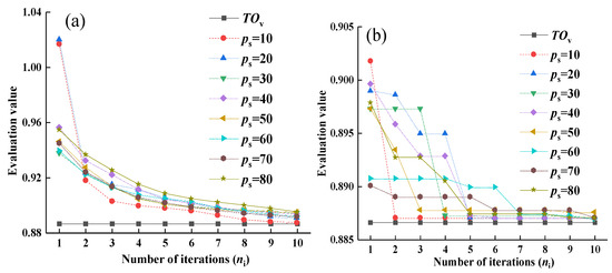
Figure 3.
Effects of population size and number of iterations on the population. (a) Optimal value of population (b) Average value of population.
Figure 3b shows that the average value (Av) curve of the population gradually becomes gentle when the population size (ps) increases and Av gradually decreases when the number of iterations (ni) increases. When the ps is 20, the initial deviation is too large, but when ps r is greater than 30, the population can achieve better calculation results.
By comparing the number of six populations, it is found that the increase in population size (ps) helps to quickly find the theoretical optimal value (TOv). By comparing the number of 10 iterations, it is found that the number of iterations (ni) is helpful to the overall optimization of the population. In order to ensure the accuracy of the calculation and considering that the calculation time is linearly positively correlated with the ps and ni, the calculation in this paper will use ps is 50 and ni is 10 as the calculation data.
5.3. Effects of Crossover Operator and Mutation Operator on Population
Considering the randomness of crossover and mutation, the effects of crossover operator (Oc) from 0.1 to 1 and mutation operator (Om) from 0.05 to 0.5 on population parameters is analyzed.
Figure 4a shows that the optimal value (Ov) curve of the population and the average value (Av) curve of the population gradually approach the theoretical optimal value (TOv) when the crossover operator (Oc) increases. When Oc is 0.7, 0.8 and 0.9, Av and Ov reach TOv at the same time. However, when the Oc is 1, the parameters of the optimal profile group of each generation are destroyed, so that Av and Ov cannot reach TOv.
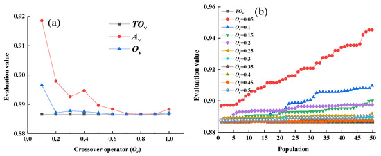
Figure 4.
Effects of population on crossover operator. (a) Optimal value and average value (b) Population value.
Figure 4b shows that the population value curve is gradually gentle when the crossover operator (Oc) increases. Due to the fact that the more sufficient the crossover, the more comprehensive is the population screening, the easier it is to find the theoretical optimal value (TOv). However, when the Oc is 1, the optimal value (Ov) of each calculation is destroyed such that Ov cannot reach TOv.
Figure 5a shows that the optimal value (Ov) curve of the population and the average value (Av) curve of the population gradually approach the theoretical optimal value (TOv) when the mutation operator (Om) increases. When Om is 0.15 and 0.2, Av and Ov reach TOv at the same time. However, when Om increases from 0.2 to 0.3, Av cannot reach TOv; Ov is still in the optimal solution. The optimal profile group parameters of each generation are destroyed, so that Av and Ov cannot reach TOv.
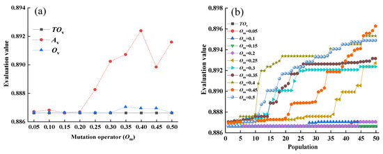
Figure 5.
Effects of population on mutation operator. (a) Optimal value and average value (b) Population value.
Figure 5b shows that the population value curve is gradually gentle when the mutation operator (Om) decreases because the mutation is to optimize the population by introducing new values when the crossover has little effect on the population optimization. However, when Om exceeds 0.3, the optimization effect of crossover on the population will be reduced; the optimal value (Ov) will be far away from the theoretical optimal value (TOv).
By comparing the effects of 10 crossover operators (Oc) and 10 mutation operators (Om) on the calculation, considering the accuracy of the calculation, Oc of 0.8 and Om of 0.15 are the calculation parameters.
5.4. Optimization Result
The optimal profile design parameters of the improved GHH profile are found: the inner radius of the male rotor (Ri) is 26 mm, the outer radius of the female rotor (Ro) is 0.4 mm, the protection angle (θ) is 0 and the radius of elliptic arc (a) is 10 mm.
It can be observed that the tooth thickness of the female rotor decreased while that of the male rotor increased on the tooth profile after optimization in Figure 6. On the geometric characteristic parameters, the length of the contact line is 178.89, which increased by 1.57%; the blow hole area is 1.39, which is reduced by 54.8%, and the area utilization rate is 0.458, which increased by 0.32%.
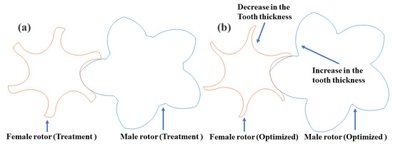
Figure 6.
Rotor diagram. (a) Treatment group profile (b) Optimized group profile.
6. CFD Simulation Results
The calculated optimization results only analyze the numerical changes of geometric characteristics. In order to understand the effects of the rotor before and after optimization more intuitively, the mesh model of the twin-screw component is established, and the fluid–solid coupling method is used to analyze the operation state of the rotor before and after optimization.
6.1. Model and Control Method
The working fluid is ideal gas, and the standard k-epsilon model is used to simulate the fluid turbulence model. The inlet condition is set as pressure inlet, the outlet condition is set as pressure outlet and the other boundary surfaces are set as wall surfaces. The speed linear solver uses conjugate gradient squared. The pressure linear solver uses algebraic multi-grid solver. While the simple method was used to solve the pressure–velocity coupling problem, numeric scheme is upwind, sweeps is 50, linear solver tolerance is 0.1 and diagonal relaxation is 0.3.
The screw compressor model consists of five parts: male rotor, female rotor, cylinder, suction port and exhaust port, as shown in Figure 7. It is assumed that the pressure, temperature and density in the chamber are uniform within the control volume. Using the transient ns equation to solve the mass and kinetic energy conservation [25]:
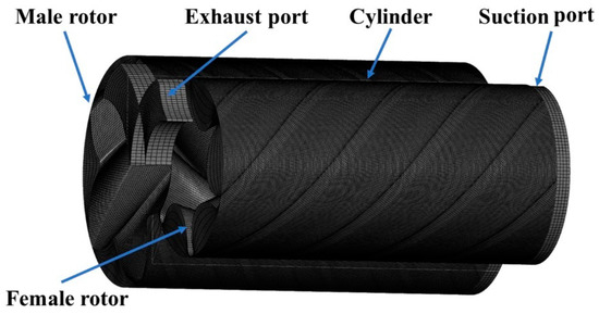
Figure 7.
Simulation model of screw compressor.
Continuity:
Kinetic energy:
Stress tensor:
In the formula: ρ represents average local fluid density, υ represents fluid velocity, υσ represents mesh velocity, n represents surface normal, σ represents surface of control volume, Ω(t) represents control volume as a function of time, t represents time, τij represents effective shear stress, f represents body force, μ represents dynamic viscosity, μt represents turbulent dynamic viscosity, δij represents Kronecker delta and p represents static pressure.
6.2. Mesh Independent Verification and Time Independent Verification
Before calculation, the simulation model needs to determine the parameters of the rotor, as shown in Table 5.
Table 5.
Parameters of the rotor.
Based on the time step of 8 × 10⁻⁵ s, the mesh independent verification is carried out to compare the simulation accuracy under different mesh sizes. The results show that the difference between the simulation results is only 1.5% at 0.5 mm and 0.25 mm mesh size; see Table 6. This indicates that mesh independent results could be achieved with the mesh of 0.5 mm.
Table 6.
Mesh independent verification.
Based on the mesh sizes of 0.5, the time independent verification is carried out to compare the simulation accuracy under different time steps. The results show that the difference between the simulation results is only 1.2% at 8 × 10⁻⁵ s and 4 × 10⁻⁵ s time steps in Table 7. This indicates that time step independent results could be achieved with the time of 8 × 10⁻⁵ s.
Table 7.
Time independent verification.
6.3. Optimization Comparison
Figure 8a shows that the pressure of the rotor chamber before optimization is lower than that after optimization at the same rotation angle. The reason is that when the contact line length and area utilization rate change little, the blow hole area of the optimized rotor is reduced by 54%, and the gas mass leaking from the high-pressure chamber to the low-pressure chamber on the compression side is reduced by 54% under the same pressure, so that the optimized rotor chamber pressure is slightly higher than that before optimization. The reduction can be observed in Figure 8b.
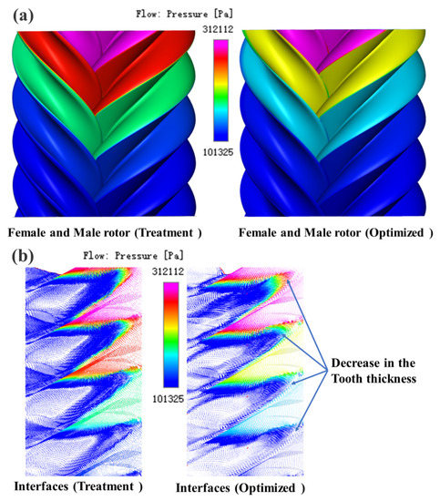
Figure 8.
Comparison of treatment group and optimized group. (a) Rotor pressure (b) Interface pressure.
It can be seen from Figure 9 that when the rotor rotates stably, the average mass flow rates of the rotor exhaust before and after optimization are 0.0229 and 0.0240 kg/s, respectively, an increase of 5.2%. The maximum values of exhaust mass flow rates are 0.0448 and 0.0446, respectively, an increase of 3.2%. The optimized leakage decreases and the mass flow increases, which proves the effectiveness of the optimization model.
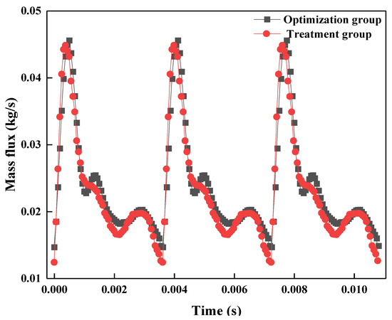
Figure 9.
Rotor exhaust port mass flow variation diagram.
7. Conclusions
In this paper, a mathematical model of profile parameter optimization based on BP neural network and genetic algorithm is established. Because the original calculation time is long, the BP neural network database is established. The geometric characteristics of a twin-screw compressor are interpolated and extrapolated to verify the predictive ability of the database. Then, the neural network database is brought into the genetic algorithm to find the optimal profile parameter group. The calculated optimal group and the treatment group are compared with the rotor performance in the simulation model. The following conclusions are drawn:
(1) The BP neural network for predicting the geometric characteristics of a twin-screw compressor is established. The effects of three training methods and four hidden neurons on data prediction accuracy are compared. The error between the predicted data and the actual value is within 1.5%, and the calculation time is shortened by 92.8%.
(2) The genetic algorithm is used to determine the optimal GHH profile parameters in specific situations. After optimization, the contact line is increased by 1.57%, the blow hole area is reduced by 54.8% and the area utilization rate is increased by 0.32%.
(3) The simulation model is used to verify the optimized mathematical model. The average mass flow rates of the rotor exhaust end before and after optimization were 0.0229 and 0.0240 kg/s, respectively, an increase of 5.2%. The maximum mass flow rates at the exhaust end were 0.0448 and 0.0460 kg/s, respectively, an increase of 3.2%.
8. Prospect
This article mainly provides an optimization method for the profile, considering only the sealing performance and volumetric performance of the rotor without considering other influencing factors, such as stress. For example, due to not considering the influence of force, the thickness of the tooth tip of the optimized female rotor is significantly reduced. When the pressure difference in the chamber is too large, it may cause the rotor to deform under the action of force. In the next stage, the influence of other factors on the rotor will be added to the calculation to enrich the evaluation mechanism of the profile.
Author Contributions
Software, D.Z.; Data curation, W.Z.; Writing—original draft, Q.Q.; Writing—review & editing, T.W. All authors have read and agreed to the published version of the manuscript.
Funding
National Natural Science Foundation of China (No. 52006201).
Data Availability Statement
Not applicable.
Conflicts of Interest
The authors declare no conflict of interest.
Nomenclature
| a | radius of the elliptic arc (mm) |
| A | area between teeth (mm2) |
| A1 | cross-sectional area of the single male groove (mm2) |
| A2 | cross-sectional area of the single female groove (mm2) |
| Ab | blow hole area (mm2) |
| Abt | blow hole area of treatment group (mm2) |
| Abo | blow hole area of optimization group (mm2) |
| Av | average value |
| BP | back-propagation |
| c | step length |
| Cn | area utilization rate |
| Cnt | area utilization rate treatment group |
| Cno | area utilization rate optimization group |
| D1 | diameter of the positive rotor (mm) |
| f | body force |
| H | number of hidden neurons |
| I | effects coefficient |
| IC | effects coefficient of area utilization rate |
| IL | effects coefficient of contact line |
| IA | effects coefficient of blow hole area |
| k | sample value |
| ki’ | average value of the sample |
| ki’’ | predicted sample value |
| L | length of the contact line (mm) |
| Lt | length of the contact line of treatment group (mm) |
| Lo | length of the contact line of optimization group (mm) |
| M | number of input neurons |
| Mv | minimum value |
| MSE | mean square error |
| N | number of output neurons |
| n | surface normal |
| ni | number of iterations |
| Ov | optimal value |
| Oc | crossover operator |
| Om | mutation operator |
| p | static pressure (Pa) |
| ps | population size |
| R | goodness-of-fitting index |
| Ri | inner radiuses of the male rotor (mm) |
| Ro | outer radius of the female rotor (mm) |
| R1 | pitch radius of male rotor (mm) |
| R2 | pitch radius of female rotor (mm) |
| s | sample size |
| t | time |
| ti, ti+1 | starting point and end point parameters of the curve |
| TOv | theoretical optimal value |
| Vmax | maximum geometric characteristics |
| Vmin | minimum geometric characteristics |
| xi, yi, zi | curve parameter equation |
| xi’, yi’ | derivative of the curve equation to the parameter |
| Z1 | number of male rotor teeth |
| Zb | the leakage surface |
| θ | protection angle (°) |
| ρ | average local fluid density (kg/m3) |
| υ | fluid velocity |
| υσ | mesh velocity |
| σ | surface of control volume |
| Ω(t) | control volume as a function of time |
| τ | screw lead (mm) |
| τij | effective shear stress |
| μ | dynamic viscosity (Pa/s) |
| μt | turbulent dynamic viscosity (Pa/s) |
| δij | Kronecker delta |
References
- Guo, Y.; Wang, T.; Liu, X.; Zhang, M.; Peng, X. Mathematical modelling and design of the ionic liquid compressor for the hydrogen refuelling station. Int. J. Energy Res. 2022, 46, 19123–19137. [Google Scholar] [CrossRef]
- Zhang, Z.; Qiu, H.; Li, D.; He, Z.; Xing, Z.; Wu, L. Development of ultra-high-efficiency medium-capacity chillers with two-stage compression and interstage vapor injection technologies. Energies 2022, 15, 9562. [Google Scholar] [CrossRef]
- Rey Martínez, F.J.; San José Alonso, J.F.; Velasco Gómez, E.; Tejero González, A.; Esquivias, P.M.; Rey Hernández, J.M. Energy consumption reduction of a chiller plant by adding evaporative pads to decrease condensation temperature. Energies 2020, 13, 2218. [Google Scholar] [CrossRef]
- Tao, W.; Guo, Y.; He, Z.; Peng, X. Investigation on the delayed closure of the suction valve in the refrigerator compressor by FSI modeling. Int. J. Refrig. 2018, 91, 111–121. [Google Scholar] [CrossRef]
- Wu, H.; Liu, J.; Shen, Y.; Liang, M.; Zhang, B. Research on performance of variable-lead rotor twin screw compressor. Energies 2021, 14, 6970. [Google Scholar] [CrossRef]
- Wu, H.; Huang, H.; Zhang, B.; Xiong, B.; Lin, K. CFD simulation and experimental study of working process of screw refrigeration compressor with R134a. Energies 2019, 12, 2054. [Google Scholar] [CrossRef]
- Gan, R.; Li, B.; Tang, T.; Liu, S.; Chu, J.; Yang, G. Noise optimization of multi-stage orifice plates based on RBF neural network response surface and adaptive NSGA-II. Ann. Nucl. Energy 2022, 178, 109372. [Google Scholar] [CrossRef]
- Wang, Y.; Chen, X.; Li, C.; Yu, Y.; Zhou, G.; Wang, C.; Zhao, W. Temperature prediction of lithium-ion battery based on artificial neural network model. Appl. Therm. Eng. 2023, 228, 120482. [Google Scholar] [CrossRef]
- Sirignano, J.; MacArt, J.; Spiliopoulos, K. PDE-constrained models with neural network terms: Optimization and global convergence. J. Comput. Phys. 2023, 481, 112016. [Google Scholar] [CrossRef]
- Holland, J.H. Adaptation in Natural and Artificial Systems; University of Michigan Press: Ann Arbor, MI, USA, 1975. [Google Scholar]
- Hernandez, C.; Lara, J.; Arjona, M.A.; Melgoza-Vazquez, E. Multi-objective electromagnetic design optimization of a power transformer using 3d finite element analysis, response surface methodology, and the third generation non-sorting genetic algorithm. Energies 2023, 16, 2248. [Google Scholar] [CrossRef]
- Ahmed, F.; Zhu, S.; Yu, G.; Luo, E. A potent numerical model coupled with multi-objective NSGA-II algorithm for the optimal design of stirling engine. Energy 2022, 247, 123468. [Google Scholar] [CrossRef]
- Wu, X.; Wang, L.; Chen, B.; Feng, Z.; Qin, Y.; Liu, Q.; Liu, Y. Multi-objective optimization of shield construction parameters based on random forests and NSGA-II. Adv. Eng. Inform. 2022, 54, 101751. [Google Scholar] [CrossRef]
- Fazlinezhad, A.; Fattahi, M.; Tavakoli-Chaleshtori, R.; Rezaveisi, H. Sensitivity analysis and multi-objective optimization of oxidative dehydrogenation of propane in a fixed-bed reactor over vanadium/graphene for propylene production. Chem. Eng. Technol. 2022, 45, 309–318. [Google Scholar] [CrossRef]
- Cornwell, E.Y.; Waite, L.J. Social disconnectedness, perceived isolation, and health among older adults. J. Health Soc. Behav. 2009, 50, 31–48. [Google Scholar] [CrossRef]
- Ma, S.-B.; Kim, S.; Kim, J.-H. Optimization Design of a Two-Vane Pump for Wastewater Treatment Using Machine-Learning-Based Surrogate Modeling. Processes 2020, 8, 1170. [Google Scholar] [CrossRef]
- Sun, Z.; Tang, F.; Shi, L.; Liu, H. Multi-conditional optimization of a high-specific-speed axial flow pump impeller based on machine learning. Machines 2022, 10, 1037. [Google Scholar] [CrossRef]
- Li, Y.; Zhou, S.; Liu, J.; Tong, J.; Dang, J.; Yang, F.; Ouyang, M. Multi-objective optimization of the Atkinson cycle gasoline engine using NSGA III coupled with support vector machine and back-propagation algorithm. Energy 2023, 262, 125262. [Google Scholar] [CrossRef]
- Byeon, S.-S.; Lee, J.-Y.; Kim, Y.-J. Performance characteristics of a 4 × 6 oil-free twin-screw compressor. Energies 2017, 10, 945. [Google Scholar] [CrossRef]
- Tian, Y.; Geng, Y.; Yuan, H.; Zhao, Z. Investigation on water injection characteristics and its influence on the performance of twin-screw steam compressor. Energy 2022, 259, 124886. [Google Scholar] [CrossRef]
- He, Z.; Wang, T.; Wang, X.; Peng, X.; Xing, Z. Experimental investigation into the effect of oil injection on the performance of a variable speed twin-screw compressor. Energies 2018, 11, 1342. [Google Scholar] [CrossRef]
- Wang, J.; Zhao, X.; Zhao, L.; Pan, S.; Wang, Z.; Cui, D.; Geng, M. Clearance distribution design and thermal deformation analysis of variable-pitch screw rotors for twin-screw vacuum pumps. Vacuum 2023, 211, 111936. [Google Scholar] [CrossRef]
- Wang, J.; Zhao, L.; Zhao, X.; Pan, S.; Wang, Z.; Cui, D.; Geng, M. Optimal design and development of two-segment variable-pitch screw rotors for twin-screw vacuum pumps. Vacuum 2022, 203, 111254. [Google Scholar] [CrossRef]
- Rumelhart, D.E.; Hinton, G.E.; Williams, R.J. Learning representations by back propagating errors. Nature 1986, 323, 533–536. [Google Scholar] [CrossRef]
- Ding, H.; Visser, F.C.; Jiang, Y.; Furmanczyk, M. Demonstration and validation of a 3d CFD simulation tool predicting pump performance and cavitation for industrial applications. J. Fluids Eng. 2011, 131, 011101. [Google Scholar] [CrossRef]


Disclaimer/Publisher’s Note: The statements, opinions and data contained in all publications are solely those of the individual author(s) and contributor(s) and not of MDPI and/or the editor(s). MDPI and/or the editor(s) disclaim responsibility for any injury to people or property resulting from any ideas, methods, instructions or products referred to in the content. |
© 2023 by the authors. Licensee MDPI, Basel, Switzerland. This article is an open access article distributed under the terms and conditions of the Creative Commons Attribution (CC BY) license (https://creativecommons.org/licenses/by/4.0/).