Neuromodel of an Eddy Current Brake for Load Emulation

Abstract

The eddy current brake (ECB) is an electromechanical energy conversion device that can be used as a load emulator to load a motor according to the intended load scenario. However, conducting an analysis in the time domain is difficult due to its complex behavior involving mechanical, electrical, and magnetic phenomena. The challenges with the time domain analysis of the ECB require new modeling approaches that provide reliability, robustness, and controllability over a wide speed interval. If the ECB can be modeled with high accuracy, it can be controlled like a load emulator that can simulate nonlinear industrial loads. This paper describes a neuromodeling approach taken to develop an ECB. The nonlinear characteristic of the brake system was modeled with a high performance by using an artificial neural network (ANN), which is a potent nonlinear system identification tool. Several characteristics of a designed and optimized brake system undergoing various excitation currents in whole speed regions are described and verified experimentally. Eventually, an electromechanical brake system is proposed that aims to provide the required linear or nonlinear load model dynamics throughout an emulation process in line with the obtained neuromodel. To identify the most suitable ANN architecture for the problem, various ANN configurations, ranging from 1 neuron to 20 neurons in the hidden layer, as well as a statistical approach that differs from the existing literature, are presented. Additionally, the suggested model’s scalability is discussed.

1. Introduction

The number of industrial loads exhibiting a nonlinear load profile has increased coherently with the evolution of industrial processes. Therefore, the traditional controller structures used in drives have been updated by adaptive, robust, and intelligent algorithms [1]. Owing to their advantages on time-varying and nonlinear industrial loads, these controllers are preferred in the modern industrial electrical drive. In order to design these algorithms in a laboratory environment, a linear or nonlinear load emulator that can simulate the desired load profile is required [2]. Load emulators provide opportunities to realistically model and test electrical drives and ensure nonlinear or linear load scenarios for the design of advanced control techniques [1,2].

Another critical issue in modern industrial drive systems is the selection of electric motors. It is essential to know both the nonlinear and linear load torque and power profile to determine the operational quantities of an electrical motor [2,3,4]. The dynamical behavior of an electrical machine is crucial since the motor does not operate at a fixed power or torque practically at all times. Electrical motors may be subjected to both linear and nonlinear loads. Therefore, they must also be capable of delivering the desired drive torque or power for nonlinear loads exhibiting variable demand. To ensure that the proper electric motor is selected for an industrial drive system, numerical and physical simulations of the real system using a load emulator are essential and necessary [1,2,3,4,5,6,7,8]. The load emulator can be cosimulated with the mathematical or finite element model of the motor. Moreover, conventional controller structures used in drives can be modified by implementing adaptive, robust, and intelligent algorithms [8].

ECBs are widely utilized for retarding linear and rotating systems such as a vehicle drive train, high-speed train, and rollercoaster. Eddy current brakes were first proposed by Japanese scientists in 1990 as a supplement to the main rail brake to reduce the speed of high-speed trains in emergency situations. These brakes can be categorized as permanent magnet eddy current brakes or electromagnetic eddy current brakes classified by their excitation mode. According to different application fields, they can be divided into magnetic couplers, magnetic retarders, magnetic couplings, magnetic retarders/reducers/brakes, magnetic dampers, etc. Additionally, they are complementary to friction brakes in semitrailer trucks to assist in preventing brake wear and overheating [9]. Most dynamometers and many motor dynamometers use an ECB to provide an electrically tunable load on the motor, as seen in Figure 1. Unlike a conventional brake system, an ECB is frictionless and more durable at the braking stage. For this reason, the brake response is more sustainable and requires less maintenance [2,4,9]. Since they do not absorb energy, their radiated heat can be removed from the system quickly. The system can be equipped with forced air ventilation or a liquid heat exchanger to reinforce cooling.

ECBs usually use the rotational or translational movement of a conductive disk between two oppositely polarized magnets to induce an electromotive force in the conductive material [10]. Eddy currents are produced inside the conductive disk, mostly coming across to the pole projection area, when a rotational or translational conductive material is subjected to a time-invariant magnetic flux. Eddy currents and a time-invariant magnetic flux interact to produce a braking torque, in accordance with Lorenz’s law [11]. Windings can be used as a magnetic field source in braking systems instead of magnets. In this case, the windings are fed with a direct current, and the conductive disc is connected to a rotating shaft. A braking force occurs due to the change in the magnetic flux on the disc over time [12]. The braking torque of the ECB can be adjusted by changing the excitation current of the ECB [13]. Therefore, it is possible to implement a mechanical load emulator that provides the desired torque by using a current-controlled eddy current brake. Recent studies in the literature have generally focused on increasing the braking force of ECBs and low friction, low inertia brake designs [14,15]. While these studies contributed greatly to eddy current brake designs, they did not provide an insight into their modeling and simplified analysis.

In this study, the design and control of a dynamobrake system is presented, which attempts to maintain the required load model dynamics throughout the emulation. The loading machine in the dynamobrake system is chosen as the ECB. In order to accurately drive the ECB as a mechanical load emulator over a wide speed range, its mathematical model must be known with high accuracy. Because of its complicated behavior involving mechanical, electrical, and magnetic phenomena, a time-domain analysis of the brake system and deriving the dynamic equations of an ECB are practically unfeasible. The challenges with the time domain analysis of ECBs necessitate the application of new modeling approaches that allow reliability, robustness, and controllability over wide speed ranges. For this purpose, the nonlinear dynamic characteristics of the ECB have been modeled with an artificial neural network (ANN), which is a nonlinear system identification method providing high accuracy. Different than the previous studies, the proposed approach provides the following:

(1) Different operational characteristics of designed and optimized ECBs for various excitation currents under high, low, and medium speed regions are achieved experimentally and presented.

(2) To choose the best ANN architecture for the ECB modeling problem, various ANN configurations, ranging from 1 neuron to 20 neurons in the hidden layer, as well as a statistical approach that differs from the existing literature, are presented.

(3) It is discussed how the suggested ANN modeling approach may even be scaled to similar ECB systems.

(4) Finally, the performance of the proposed load emulator system for frequently encountered load scenarios for electric motors used in industrial drive systems is discussed.

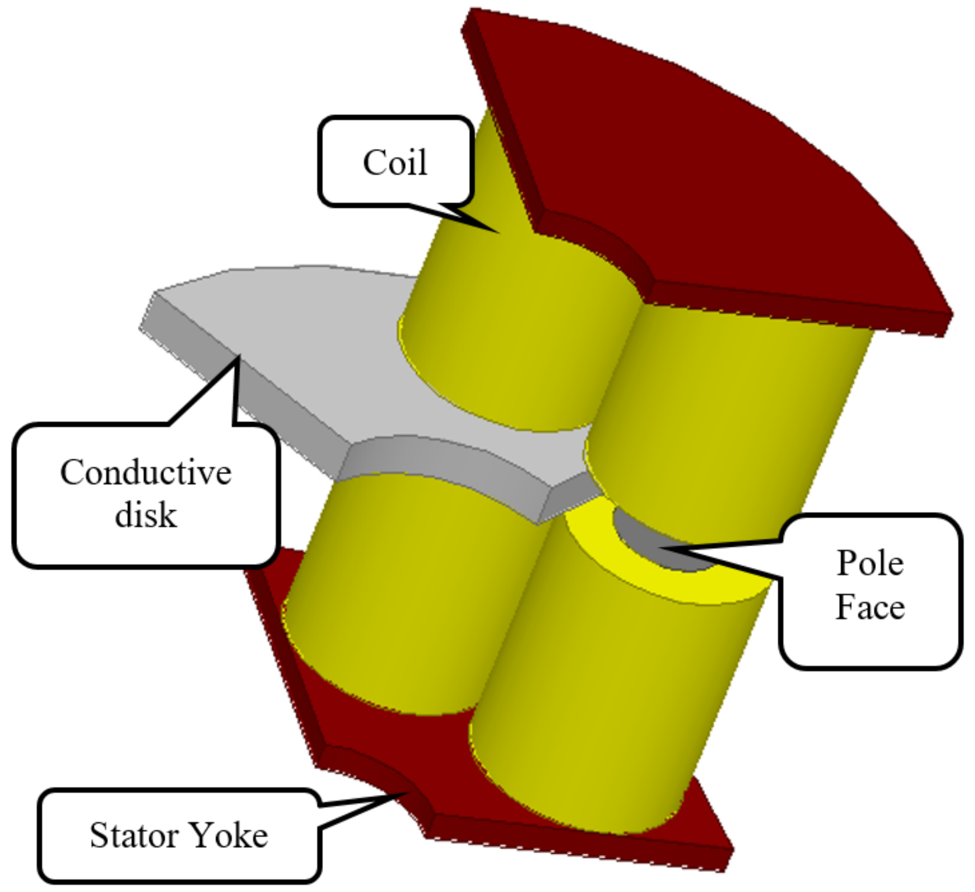
2. Analytical Torque Expression of ECB

An ECB is made up of a conductive disk coupled to a rotational mechanical energy source and a fixed magnetic flux source, such as an electromagnet or permanent magnet. The conductive material is subjected to a time-varying magnetic flux density as a function of rotation, which may be described by Lenz’s (1) law, where E denotes the electric field strength and B denotes the magnetic flux density [12]:

$$\nabla \times \overrightarrow{E}=-\frac{\partial \overrightarrow{B}}{\partial t}$$

(1)

Because of Ohm’s law (2), where J is the current density and $\sigma$ represents conductivity, an electric field generates current. These eddy currents move in a loop along the material [12]:

$$\overrightarrow{J}=\sigma ·\overrightarrow{E}$$

(2)

The elemental braking force ($\Delta$F) resulting from the interaction between the eddy currents and magnetic flux density and the generated braking torque (T) are provided in (3) and (4), where r is the radius of the disc; g is the air-gap thickness; e is the disc thickness; and $R_{inner}$ and $R_{outer}$ are the inner and outer radii of the disc, respectively [13]:

$$\Delta \overrightarrow{F}=\overrightarrow{J}\times \overrightarrow{B}$$

(3)

$$T={\int }_g^{g+e}dz{\int }_0^{2\pi }d\theta {\int }_{R_{inner}}^{R_{outer}}r·\Delta F_{\theta }·r·dr$$

(4)

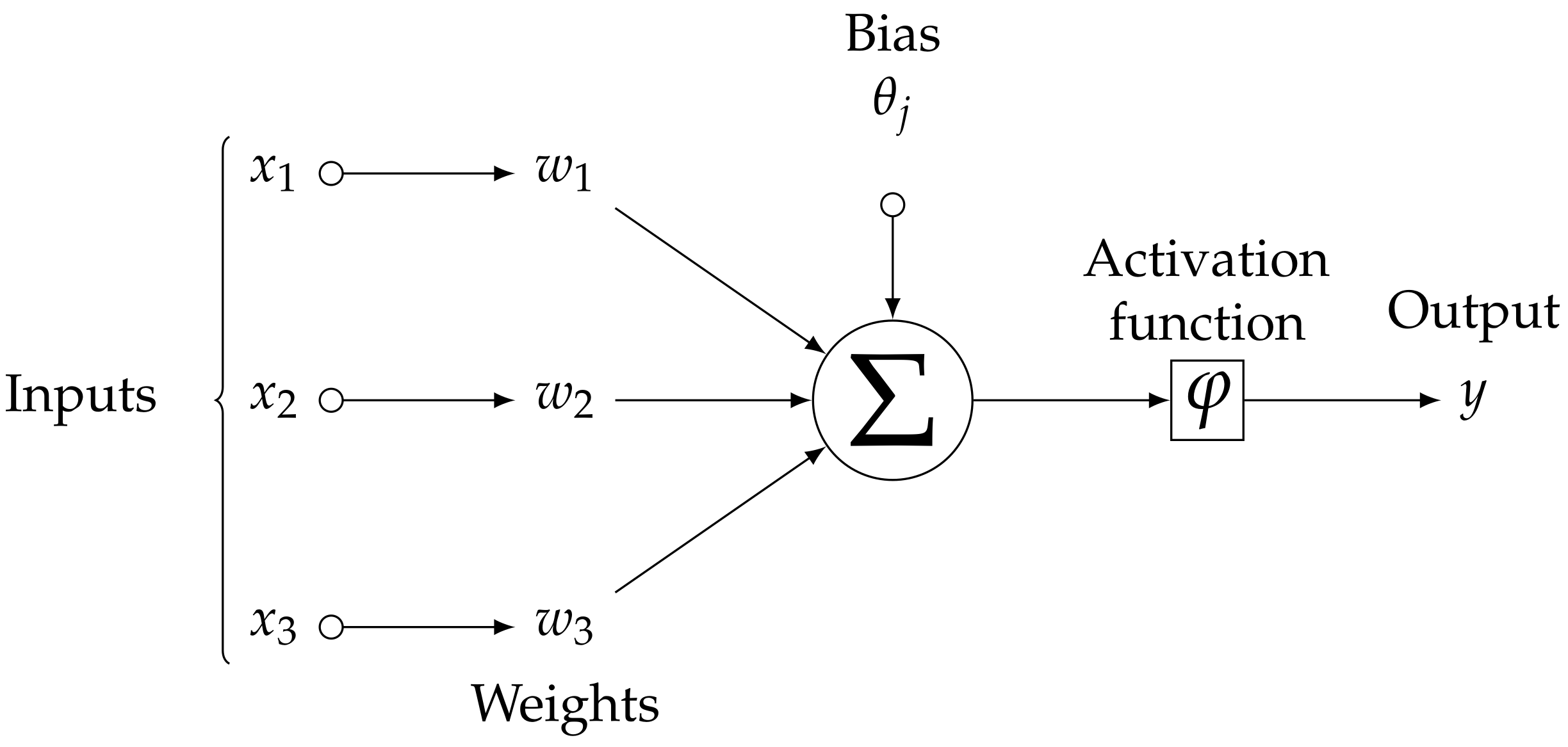
3. Artificial Neural Network for Nonlinear System Modeling

In the modeling of nonlinear systems and system identification, artificial neural networks (ANN) that are modeled after biological neurons are frequently utilized. An artificial neural network typically has three layers: an input layer, one or more hidden layers, and an output layer. Numerous neurons make up each layer, and the user determines the number of layers and neurons in each layer based on the size of the issue. All the neurons are connected to each other and imitate the biological nervous system [16,17,18].

ANNs do not contain any tangible details concerning the system. Instead, it is taught to understand the relationship between the system’s inputs and outputs using a sample dataset. Training, validation, and testing are the three main processes that may be used to complete an ANN. Three subsets of the sample dataset were created randomly for this purpose. The magnitude of the training subsets is often significantly bigger than the rest. Validation and testing may be performed with the remaining sets [17,18,19]. An examination of the single neuron’s training process is shown in Figure 2.

The training set is used to train the ANN initially. Any input-related weights are given random real values. Consequently, the initial input and output are where the process begins. Each input ($x_i$) is multiplied by its associated weight ($w_i$), and the weighted inputs are summed as stated in (5) [17]:

$$\sum _{i=1}^n\left(x_i·w_i\right)=x_1·w_1+x_2·w_2+x_3·w_3+\cdots +x_n·w_n$$

(5)

An activation function uses the weighted sum in its calculations. A sigmoid function such as the one in (6) [17] is commonly used as the activation function:

$$f\left(x\right)=\frac{1}{1+e^{-x}}$$

(6)

A learning algorithm is used to compute and propagate back the differences in the output between the neuron’s actual output and expected output. The weights of such an ANN are updated in accordance with a selected learning technique, and it is known as a feed-forward (backward propagation) neural network. The selected learning algorithm makes an effort to reduce the discrepancy between the actual output and the expected output. Algorithms for learning frequently employ a gradient descent. The Levenberg–Marquardt algorithm (LMA), which stands out among learning algorithms, is typically utilized because of its speed and resilience. Combining the gradient descent technique and the Gauss–Newton method yields the LMA, which may be characterized as a simple yet effective algorithm. Distinguished references [17,18,19] provide thorough information. The mean square error is typically utilized in ANN training even if other performance criteria can be defined. After the weights are updated, the process is repeated for the next set of inputs and outputs, and one training cycle of the entire dataset is called an epoch.

Depending on the complexity of the issue, an ANN may include more than one neuron per layer, along with one or more hidden layers in various technical applications. The backpropagation method in this situation changes all of the weights of the connections between the neurons and layers and covers the complete network [17,18,19,20,21,22]. Figure 3 shows a conventional neural network with a single hidden layer.

The validation stage is another crucial step, and in order to generalize it, an ANN is applied to a dataset that is different from the training dataset. Large training datasets or a lot of epochs might lead to overfitting or memorizing. To guarantee that the ANN is generalizable, the validation step should be used after the training process [20].

The third stage is the test step, which, with one exception, is very identical to the validation step but uses a different dataset from the training and validation datasets. The test phase is used with the trained and validated ANN to assess the effectiveness of the preceding stage [20]. The validation step serves as the criterion for stopping the training step.

Finally, it should be noted that the flag-related training should be stopped. This flag might be a specified error, specified error gradient, defined number of epochs, or validation tests. The number of hidden layers and the number of neurons in each layer are all user-defined parameters, and determining the ideal values often involves a trial-and-error methodology.

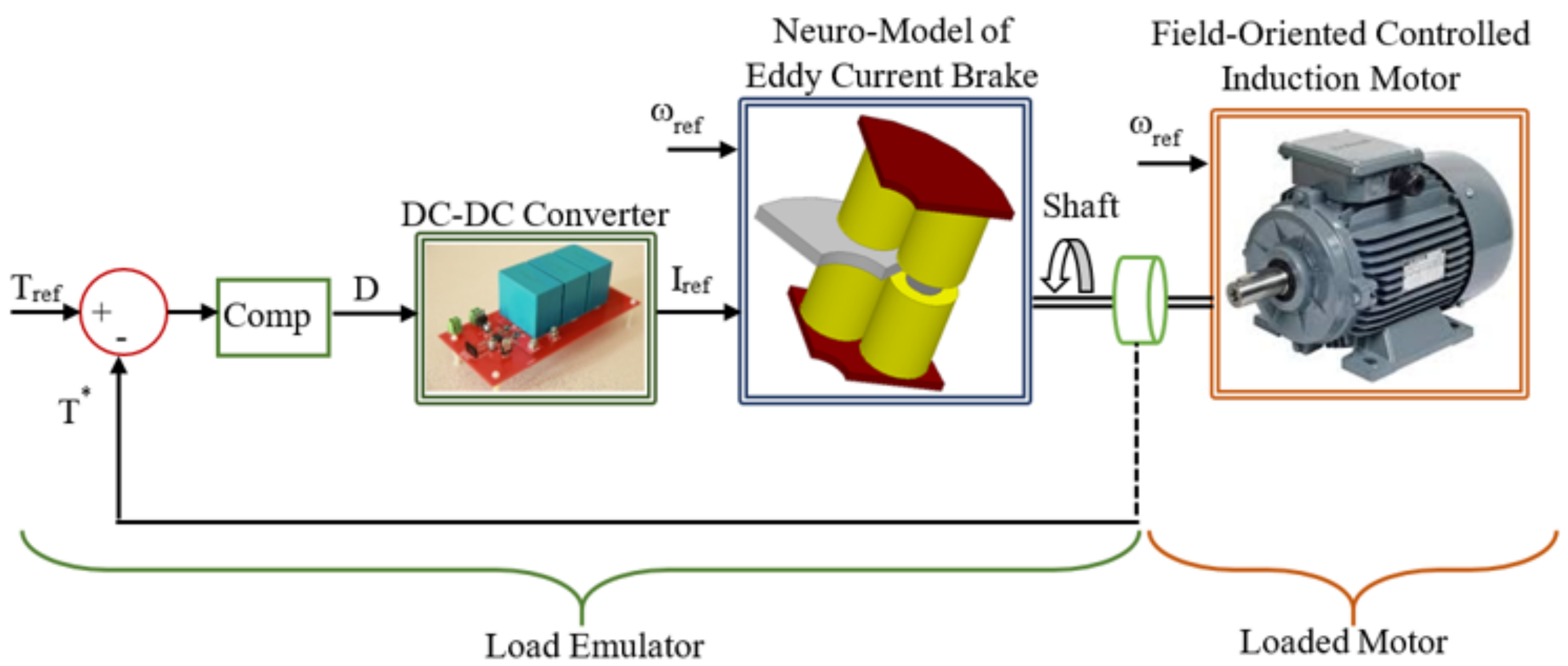
4. Implementation of the Method on ECB

This section presents an ECB’s statistical modeling approach by using an ANN. The data collection from the experimental ECB system is described first, then the application of the proposed statistical modeling approach to the ECB system is presented in detail, and finally, the applicability of the developed ECB model to other braking systems is discussed.

4.1. Experimental Setup for Collecting Data

In this study, the design was taken from a previous study conducted by the author, and the main quantities and dimensions are given

Table 1. Design parameters of ECB.

Symbol	Quantity	Value
I	Excitation current	5 A
N	Number of turns per pole	205
P	Number of pole pairs	8
${\tau }_p$	Pole width	${90}^{\circ }$
g	Air-gap width	2 mm
d	Thickness of disk	10 mm
$r_{mag}$	Radius of electromagnet	20 mm
R	Radius of disk	140 mm
${\mu }_r$	Relative permeability of conductive disk	1
$\sigma$	Conductivity of disk	18,560,000 S/m

[9,10,11].

While 7075-aluminum was used for the conductive disc in the brake system, steel-1010 was used as the magnetic material for the yokes. In order to obtain the experimental characteristics of the braking system, the ECB was mechanically coupled with a variable frequency drive (VFD)-powered induction motor. The test bench for collecting experimental data is given in Figure 4a,b.

The braking torque data generated by the ECB system at different excitation currents and different rotational speeds were collected with the USB-1608G series high-speed multifunction USB data acquisition set and DAISY Lab interface. The braking torque–speed curve and the braking power–speed curve obtained at different excitation currents are given in Figure 5a and Figure 5b, respectively.

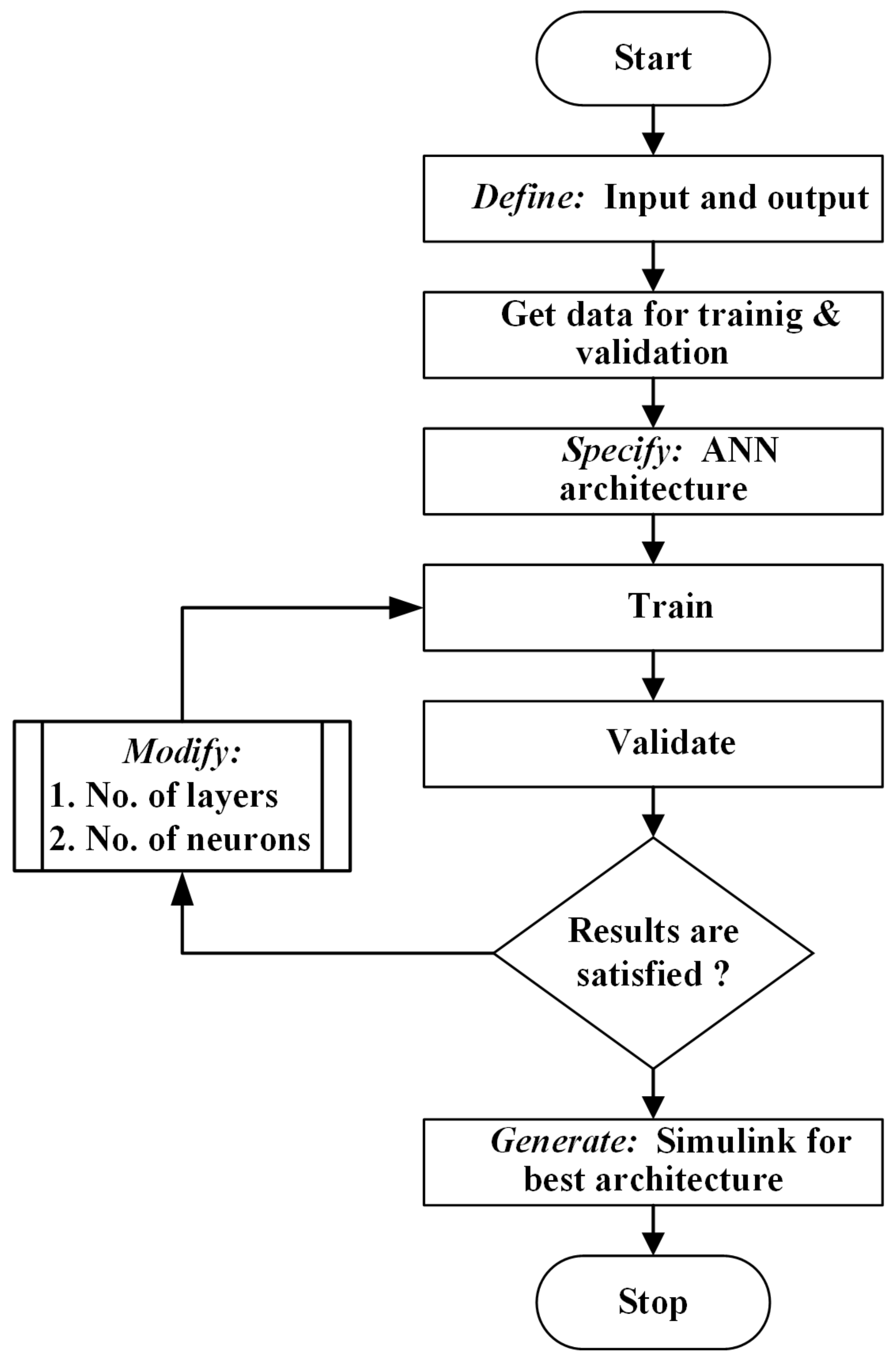
4.2. ANN Modeling of ECB

In this step of the study, an ANN was used for the torque estimation of the ECB placed in the load emulator. The nonlinear relationship between the input and output parameters was established by using the MATLAB Neural Network Toolbox. While the input parameters were used as excitation current and shaft speed, the output parameter was determined as the torque. As the established ANN had two inputs, the input layer contained two neurons, and similarly, the output layer contained one neuron. Initially, a single hidden layer was used. If the performance does not meet expectations, the number of hidden layers can be increased. In this study, the ANN was trained according to the number of sequential neurons in the hidden layer, ranging from 1 to 20. The flowchart of the proposed modeling approach is given in Figure 6. The number of training, validation, and test data in each simulation were 34 (60%), 11 (20%), and 11 (20%), respectively, and these data were randomly selected. The network was trained by using the Levenberg–Marquardt back propagation algorithm (LMA), and 50 epochs were provided as the halting criteria. Each simulation computed the mean squared errors (MSE) of the training, validation, and test data. The simulation was repeated 200 times for each number of neurons in the hidden layer, and to guarantee a reasonable comparison criteria, MSE averages and test data correlations were computed.

Table 2. The total performance indexes.

Average Train	Average Validation	Average Test	Average Test
MSE (%)	Error (%)	Error (%)	Correlation
0.2526	0.1279	0.0933	0.9114
0.0838	0.0573	0.0619	0.9017
0.0139	0.0150	0.0167	0.9764
0.0078	0.0085	0.0093	0.9844
0.0060	0.0054	0.0085	0.9857
0.0030	0.0060	0.0068	0.9901
0.0056	0.0081	0.0117	0.9837
0.0061	0.0094	0.0114	0.9813
0.0072	0.0146	0.0271	0.9730
0.0064	0.0161	0.0235	0.9639
0.0074	0.0218	0.0328	0.9560
0.0144	0.0324	0.0475	0.9347
0.0105	0.0312	0.0609	0.9166
0.0186	0.0424	0.0618	0.9061
0.0171	0.0485	0.0714	0.9088
0.0233	0.0655	0.0762	0.8921
0.0197	0.0594	0.0968	0.8616
0.0206	0.0763	0.1155	0.8492
0.0264	0.0846	0.1092	0.8552
0.0223	0.0819	0.1283	0.8313

lists the overall performance indices.

The MSE of the test data may be used to interpret the ANN’s modeling performance. It is clear from the data that an ANN with six neurons produces the lowest average mean squared error. Additionally, the identical network topology yields the second-highest average correlation of test data. The ANN depends on randomness, and it is not a fair comparison when only a few simulations are performed for each ANN architecture. All simulations begin with a set of random weights, although some simulations will have better random weights at the beginning, which leads to a higher performance. Therefore, when modeling the ECB, the simulations are run 200 times, with the averages being computed to determine the precise number of neurons needed to create the solution architecture with the highest potential performance. In light of this information, ANNs with six neurons in the hidden layer can be claimed to be more effective than the others for modeling an EBC. In addition, in ANNs with more than 20 neurons in the hidden layer, there is an increasing trend in the average mean squared errors of the test data between 10 and 20 neurons, which indicates that the average mean squared error increases as the number of neurons increases.

Therefore, there is no need to investigate the effect of the increase in the number of neurons after 20 neurons. It is not essential to simulate the ANN with more hidden layers because the average mean squared error in an ANN solution with six neurons in the hidden layer is pretty minimal. Following this point, this investigation concentrated on a six-neuron ANN in the buried layer. The simulation was run once again, but 1000 repetitions were added in between. The ANN with the best test data performance, or mean square error of the test data, was found among these 1000 trials. The ANN that performed the best was noted and used for all the data. The whole ANN output is shown in Figure 7 together with the goal values. The correlations, coefficients of determination, and mean squared errors (MSE) obtained by the neuromodel are given in

Table 3. The neuromodel’s mean squared errors (MSE), correlations, and coefficients of determination.

	MSE	R2
Train Data	0.000843	0.999468
Validation Data	0.0018	0.998963
Test Data	0.001408	0.99772
All Data	0.001147	0.99921

for all the data.

4.3. Scalability of Neuromodel of ECB

The eddy current brake does not have a linear braking torque–speed characteristic because the magnetic characteristic of the material is nonlinear and the eddy currents vary with the shaft speed. As seen in Figure 5, all eddy current brakes have a typical braking torque–speed characteristic and can be expressed in four regions:

• The system cannot have an eddy current impact if there is no relative movement between the poles and the conductive disk. This operational point crosses the axes’ origin since the poles are fixed, which means that there is “No torque at zero speed”. A time invariant flux density never produces an electric field according to Faraday’s law.
• Linear torque region: Since the breaking effect is greater as the relative speed increases while the magnetic circuit operation takes place at linear regions and produces linearly increasing magnetic fields, the reverse effect of the magnetic field produced by the eddy current at the beginning of the rotational movement is negligible against the main magnetic field generated by the poles.
• The critical speed is the velocity at which the maximum braking torque occurs. The decreasing influence of the magnetic field produced by the eddy currents becomes prominent as the relative speed rises, which causes a significant drop in the braking torque.
• High speed region: above the critical speed, angular speed rises are accompanied by higher increases in the reaction field, which lowers the overall magnetic flux density and eddy currents and causes the braking torque to constantly decrease.

It can be inferred that by including scaling factors for the current and speed at the model’s inputs and for the braking torque at the output, the neural model can be applied to all ECBs. A purposed scalable neuromodel of an ECB is illustrated in Figure 8 where $C_{\omega }$, $C_I$, and $C_T$ denote the scaling coefficients; ${\omega }_{\mathrm{ref}}$ is the speed input; $I_{\mathrm{ref}}$ is the excitation current input; T is the braking torque; and ${\omega }_{\mathrm{ref}}^{*}$, $I_{\mathrm{ref}}^{*}$, and $T^{*}$ are the scaled excitation current, speed, and torque respectively.

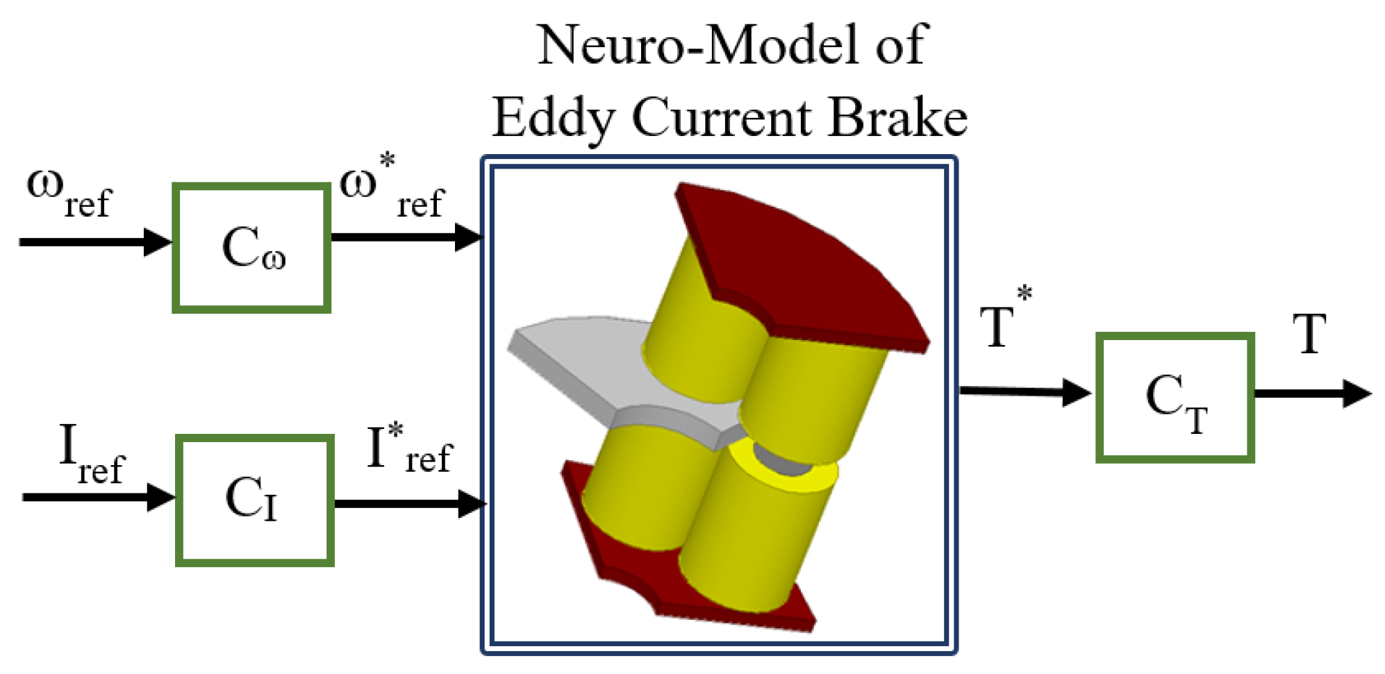
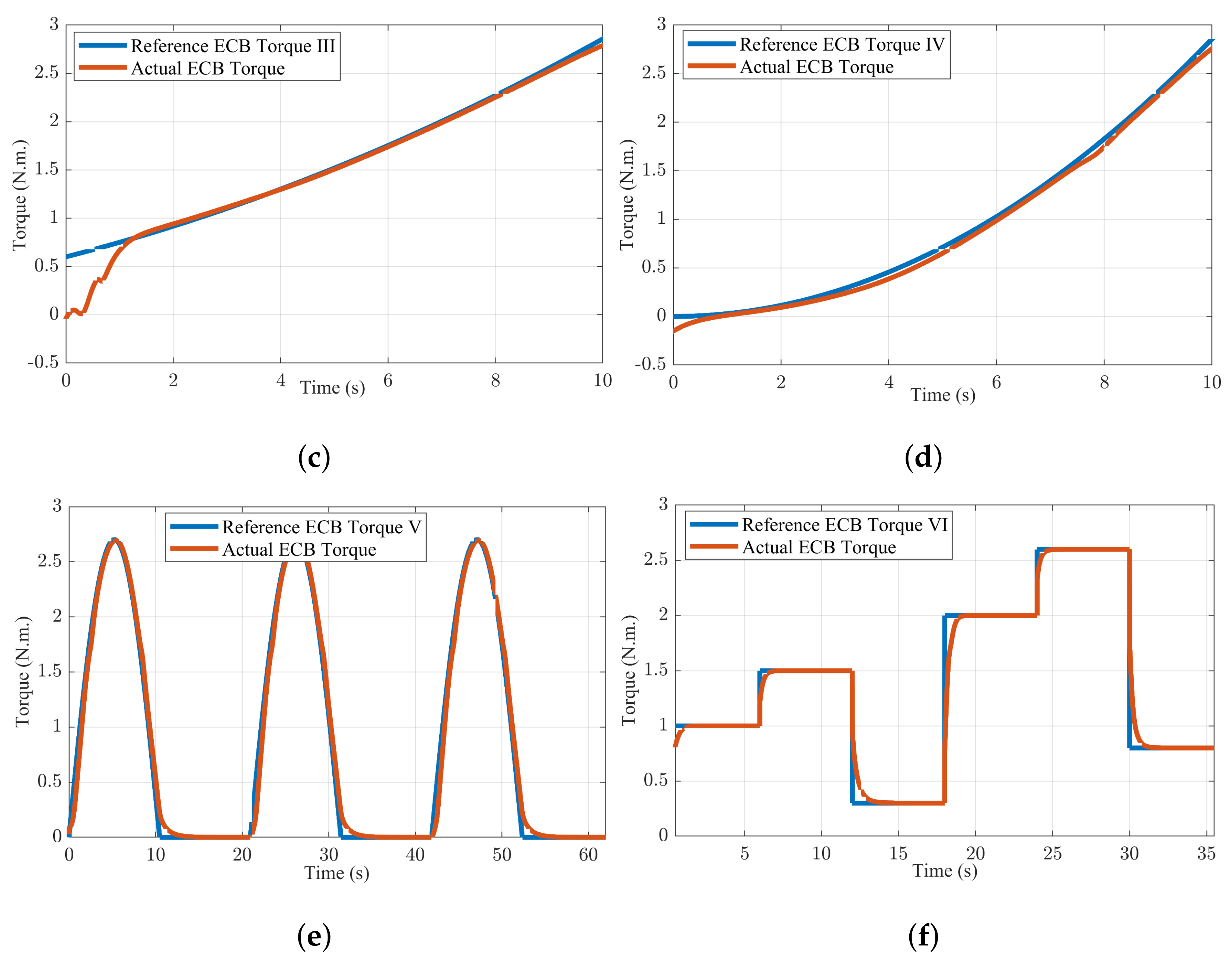
5. Investigation of Performance of Neuromodel under Different Load Scenarios

In this part of the study, the proposed dynamobrake system, controller, and vector-controlled induction motor required for a basic load emulation system are modeled in a MATLAB/Simulink environment, and the proposed simulation model is given in Figure 9. The proposed dynamobrake system for load emulation has two inputs called the excitation current ($I_{\mathrm{ref}}$) and speed (${\omega }_{\mathrm{ref}}$) reference. After the reference torque is compared with the measured torque value, the error signal is then applied to a compensator. As given in Figure 9, the shaft torque of the ECB varies with the excitation current and shaft speed. Therefore, the excitation current of the ECB must be controlled by a DC–DC converter to provide the desired torque value at the desired speed. The compensator in the proposed simulation structure sets the required duty cycle (D) in the DC–DC converter to provide the desired excitation current. The induction motor given in the model is controlled via a field-oriented controlled drive. The speed reference in the proposed system should be the same for both the induction motor and ECB on the load emulator side.

In order to analyze the performance of the proposed load emulator model, the load characteristics with a linear variation with a rotor angular velocity (I, II) and varying torques proportional to the square of the rotor angular velocity (III, IV) are defined in Figure 10. These are the most common load characteristics in industrial drive systems. Numbers (I) and (II) represent the characteristics of a first-order viscous frictional load where velocity and torques vary linearly. Number (III) represents the pump load varying with the square of the angular velocity of the load torque, while (IV) represents the second-order fan load with low friction [23].

These common load profiles were applied to the proposed load emulator model, and the results are given in Figure 11.

It can be inferred from Figure 11 that the proposed load emulator behavior was in great harmony with that of the most common load characteristics in the industrial drives. Furthermore, to obtain the performance of the proposed load emulator under aperiodic and periodic duty operation, a potential change in the load torque needs to be met in practice, as shown in Figure 11e,f. As can be seen in the figures, when the shaft speed is held constant at 2800 rpm, the reference and actual torque values were substantially equal.

Despite the fact that a visual comparison gave acceptable results, the mathematical performance of the purposed model was also calculated. Two different performance metrics were used to obtain the precision of the proposed load emulator with the most common speed–torque characteristics applied in industrial drives. The definition of the mean absolute percentage error, which is presented in (7), was used to create the first accuracy function, where k is the quantity of the torque data [11]. To calculate how closely the actual value resembles the reference value, we divided the difference between the reference and actual values by the reference value. The percentage departure from the reference values was then calculated by multiplying this value by the quantity of data (k) and dividing it by 100. The coefficient of determination is the second accuracy function. The coefficient of determination, abbreviated as $R^2$, is given as in (8), where $\overline{T_{\mathrm{neuro}}}$ denotes the mean of the torque values for the neuromodel, and $\overline{T_{\mathrm{ref}}}$ denotes the mean of the torque values for the reference.

Table 4. Accuracy results of speed–torque characterıstıcs of six different induction motors.

Load Type	Accuracy (%)	R2
1	99.9248	0.9999
2	99.9505	0.9999
3	99.8595	0.9999
4	99.8490	0.9999
5	99.6729	0.9999
6	99.7850	0.9999

provides the derived accuracy functions for each load type. The accuracy results showed that the generated neuromodel had substantially equal results with that of the actual loads for the load emulator:

$$Accuracy(\%)=100-\left(\frac{100}{k}\right)·\sum _{j=1}^k\frac{\mid T{}_{\mathrm{ref}}\left(j\right)-T{}_{\mathrm{neuro}}\left(j\right)\mid }{T{}_{\mathrm{ref}}\left(j\right)}$$

(7)

$$R^2=\frac{{\sum }_{j=1}^k\left\{T_{\mathrm{neuro}}\left(j\right)-\overline{T_{\mathrm{neuro}}}\right\}·{\sum }_{j=1}^k\left\{T_{\mathrm{ref}}\left(j\right)-\overline{T_{\mathrm{ref}}}\right\}}{\sqrt{{\left\{T_{\mathrm{neuro}}\left(j\right)-\overline{T_{\mathrm{neuro}}}\right\}}^2}·\sqrt{{\left\{T_{\mathrm{ref}}\left(j\right)-\overline{T_{\mathrm{ref}}}\right\}}^2}}$$

(8)

6. Conclusions

In this study, a dynamobrake system that can follow the required linear and nonlinear load profile dynamics during emulation is proposed. The load machine in the dynamobrake system uses an ECB with a different approach than previous load emulators. The use of the ECB as a load emulator requires its high precision modeling and robust control. The challenges with the time domain analysis of ECBs require the application of artificial intelligence approaches that allow reliability, robustness, and controllability over a wide speed range. Therefore, the nonlinear dynamic characteristic of the ECB in the load emulator was modeled with high accuracy by an artificial neural network (ANN).

An ANN with two inputs (speed and excitation current) and one output (torque) was designed as a neuromodel of an eddy current brake for load emulation. The ANN’s architecture consisted of a single hidden layer. The ECB dataset was divided into three sections: training, validation, and test. In the hidden layer, several training attempts were carried out using somewhere between 1 and 20 neurons. The performance of the neuromodel was calculated by using the mean squared error (MSE) values of each dataset and the correlations of the test data for each trial. The outcomes of the investigation stage showed that one hidden layer was sufficient. Additionally, an ANN that has six neurons in the hidden layer produces the highest results. In every trial, training came to an end after 50 epochs. Furthermore, since all eddy current brakes have a typical braking torque–speed characteristic and can be expressed in four regions, the proposed neural model can be applied to all ECBs by including scaling factors for the model’s inputs and output.

Performance tests of the obtained neural-model-based load emulator were made with the most common load profiles in the industrial drives. The obtained results were examined both visually and mathematically in six different load scenarios, and it was seen that the proposed system could follow the load profiles applied to the emulator input with up to 99.95% accuracy and a 0.9999 coefficient of determination.

References

1. Akpolat, Z.H.; Asher, G.M.; Clare, J.C. Experimental dynamometer emulation of nonlinear mechanical loads. IEEE Trans. Ind. Appl. 1999, 35, 1367–1373. [Google Scholar] [CrossRef]
2. Gulbahce, M.O.; Nak, H.; Kocabas, D.A. Design of a Mechanical Load Simulator Having an Excitation Current Controlled Eddy Current Brake. In Proceedings of the 3rd International Conference on Electric Power and Energy Conversion Systems, Istanbul, Turkey, 2–4 October 2013; pp. 1–5. [Google Scholar] [CrossRef]
3. Collins, E.R.; Huang, Y. A programmable dynamometer for testing rotating machinery using a three-phase induction machine. IEEE Trans. Energy Convers. 1994, 9, 521–527. [Google Scholar] [CrossRef]
4. Gulbahce, M.O.; Nak, H.; Kocabas, D.A. A New Approach for Temperature Rising Test of an Induction Motor Loaded by a Current Controlled Eddy Current Brake. In Proceedings of the 3rd International Conference on Electric Power and Energy Conversion Systems, Istanbul, Turkey, 2–4 October 2013; pp. 1–6. [Google Scholar] [CrossRef]
5. Arellano-Padilla, J.; Asher, G.M.; Sumner, M. Control of an AC Dynamometer for Dynamic Emulation of Mechanical Loads with Stiff and Flexible Shafts. IEEE Trans. Ind. Electron. 2006, 53, 1250–1260. [Google Scholar] [CrossRef]
6. Lee, K.; Lee, J.; Back, J.; Lee, Y.I. A Robust Emulation of Mechanical Loads Using a Disturbance-Observer. Energies 2019, 12, 2236. [Google Scholar] [CrossRef]
7. Newton, R.W.; Betz, R.E.; Penfold, H.B. Emulating Dynamic Load Characteristics Using a Dynamic Dynamometer. In Proceedings of the International Conference on Power Electronics and Drive Systems, Singapore, 21–24 February 1995; pp. 465–470. [Google Scholar]
8. Akpolat, Z.H.; Asher, G.M.; Clare, J.C. Emulation of High Bandwidth Mechanical Loads Using Vector Controlled AC Dynamometer. In Proceedings of the 8th International Power Electronics & Motion Control Conference, Prague, Czech Republic, 8–10 September 1998; pp. 133–138. [Google Scholar]
9. Gulbahce, M.O.; Kocabas, D.A.; Nayman, F. Investigation of the Effect of Pole Shape on Braking Torque for a Low Power Eddy Current Brake by Finite Elements Method. In Proceedings of the 9th International Conference on Electrical and Electronics Engineering (ELECO), Bursa, Turkey, 26–28 November 2015; pp. 263–267. [Google Scholar] [CrossRef]
10. Sinmaz, A.; Gulbahce, M.O.; Kocabas, D.A. Design and Finite Element Analysis of a Radial-Flux Salient-Pole Eddy Current Brake. In Proceedings of the 9th International Conference on Electrical and Electronics Engineering (ELECO), Bursa, Turkey, 26–28 November 2015; pp. 590–594. [Google Scholar]
11. Gulbahce, M.O.; Kocabas, D.A. A comprehensive approach to determining the speed/torque relationships of eddy current brakes. Electr. Eng. 2018, 100, 1579–1587. [Google Scholar] [CrossRef]
12. Gay, S.E.; Ehsani, M. Parametric analysis of eddy-current brake performance by 3-D finite-element analysis. IEEE Trans. Magn. 2006, 42, 319–328. [Google Scholar] [CrossRef]
13. Jeong, H.; Ji, H.; Choi, S.; Baek, J. Parametric Study of Eddy Current Brakes for Small-Scale Household Wind Turbine Systems. Energies 2021, 14, 6633. [Google Scholar] [CrossRef]
14. Wang, M.; Kou, B. Design of the Low Inertia Composite-Disc Type Magnetic Brake. In Proceedings of the 25th International Conference on Electrical Machines and Systems (ICEMS), Chiang Mai, Thailand, 29 November–2 December 2022; pp. 1–5. [Google Scholar] [CrossRef]
15. Xiang, C.; Chen, S.; Yao, M.; Gu, Y.; Yang, X. Optimization of Braking Force for Electromagnetic Track Brake Using Uniform Design. IEEE Access 2020, 8, 146065–146074. [Google Scholar] [CrossRef]
16. Hassoun, M.H. Fundamentals of Artificial Neural Networks, 1st ed.; MIT Press: Cambridge, UK, 1995. [Google Scholar]
17. Zhong, K.; Meng, Q.; Sun, M.; Luo, G. Artificial Neural Network (ANN) Modeling for Predicting Performance of SBS Modified Asphalt. Materials 2022, 15, 8695. [Google Scholar] [CrossRef] [PubMed]
18. George, A. Anastassiou Intelligent Systems: Approximation by Artificial Neural Networks, 1st ed.; Springer Press: Berlin, Germany, 2011. [Google Scholar]
19. Kevin, L.P.; Paul, E.K. Artificial Neural Networks: An Introduction, 1st ed.; SPIE Press: Washington, DC, USA, 2005. [Google Scholar]
20. Hagan, M.T.; Demuth, H.B.; Jesus, O.D. An introduction to the use of neural networks in control systems. Int. J. Robust Nonlinear Control 2002, 12, 959–985. [Google Scholar] [CrossRef]
21. Fausett, L. Fundamentals of Neural Networks: Architectures, Algorithms and Applications, 1st ed.; Prentice Hall International Press: Upper Saddle River, NJ, USA, 1994. [Google Scholar]
22. Avunduk, E.; Tumac, D.; Atalay, A.K. Prediction of roadheader performance by artificial neural network. Tunn. Undergr. Space Technol. 2014, 44, 3–9. [Google Scholar] [CrossRef]
23. Novotny, D.W.; Lipo, T.A. Vector Control and Dynamics of AC Drives, 1st ed.; Clarendon Press: Oxford, UK, 2008. [Google Scholar]
Figure 1. 3D geometry of an ECB.
Energies 16 03649 g001
Figure 2. Diagram of a single neuron.
Energies 16 03649 g002
Figure 3. Ordinary artificial neural network with a single hidden layer.
Energies 16 03649 g003
Figure 4. (a) Experimental setup of eddy current brake system; (b) eddy current brake system.
Energies 16 03649 g004
Figure 5. Braking torque (a) and braking power (b) vs. speed curves of ECB for different excitation currents.
Energies 16 03649 g005
Figure 6. The flowchart of the proposed modeling approach.
Energies 16 03649 g006
Figure 7. Scatter plots for ANN model of ECB.
Energies 16 03649 g007
Figure 8. Scalable neuromodel of eddy current brake.
Energies 16 03649 g008
Figure 9. Purposed dynamobrake system.
Energies 16 03649 g009
Figure 10. The most common load characteristics in industrial drive systems.
Energies 16 03649 g010
Figure 11. Behavior of purposed load emulator while imitating the most common load characteristics in industrial drive systems: (a) load type I; (b) load type II; (c) load type III; (d) load type IV; (e) load type V; (f) load type VI.
Energies 16 03649 g011aEnergies 16 03649 g011b