Investigation of Heat Extraction in an Enhanced Geothermal System Embedded with Fracture Networks Using the Thermal–Hydraulic–Mechanical Coupling Model

Abstract

This paper presents a numerical study on thermal energy mining from hot dry rock (HDR) using an enhanced geothermal system (EGS). In these simulations, the thermal–hydraulic–mechanical (THM) coupling model is employed on the basis of the embedded discrete fracture model. The evolution of physical fields of the fractured reservoir, including temperature field, pressure field, and stress field is studied over time, and the effects of different controllable factors, such as fracture morphology, fluid injection rate, and the distances between the injection well and producing well on the heat recovery capacity are investigated. The results show that the fracture morphology significantly influences heat extraction performance. The working fluid mainly flows along with the fracture networks, which causes locally low temperatures and low mean effective stress near fractures. The porosity and permeability increase due to the decrease in mean effective stress. For reservoir models with inclined fractures, there will be a significant decrease in the extraction temperature. In the 30th year, the decline in the heat recovery rate is 46.6%, which is much higher than the model without inclined fractures. Moreover, the increasing injection temperature barely influences the production temperature, while it significantly decreases the heat recovery of the EGS. When the injection and production well spacing is small, increasing the well spacing is an effective way to improve the thermal extraction performance of the EGS. In the model in the paper, the heat production increases up to 13.7% when the injection-production well spacing is increased from 150 m to 450 m. The results of this work could provide guidance for the optimization and operation of EGS.

1. Introduction

In the past few decades, the shortage of fossil energy and the environmental pollution caused by the utilization of fossil energy have become the focus of attention all over the world. Seeking renewable and clean energy sources, therefore, becomes imperative. The geothermal resource of hot dry rock (HDR) has aroused broad concern because of its rich reserves and its renewable, high-temperature, stable, and pollution-free characteristics. However, rocks in HDR reservoirs without natural groundwater flow are dense, having low porosity and low permeability, making it challenging to extract the stored heat [1,2]. Enhanced geothermal systems (EGS) are currently regarded as one of the most promising technologies for effectively exploiting the thermal energy of HDR [3].

The principle of EGS is to use the hydraulic fracturing process to create an artificial heat reservoir for extracting the thermal energy from low-permeability and high-temperature HDR [4]. In EGS, the cold working fluid (typically water or supercritical CO₂) circulates through the natural or engineered fractures in hot dry rocks and extracts thermal energy from reservoirs. The high-temperature fluids are returned to the surface through reinjection wells, and then the heat energy is converted into electrical energy by power generation equipment [5,6]. The heat transfer processes that occur in the subsurface may involve heat transfer (thermal), fluid flow (hydraulic), rock deformation (mechanical), and all these physical processes are interdependent [7,8]. In addition, the geometric parameters of fractures, including the length and number of fractures, fracture orientation, and fracture connectivity in the reservoir, play a vital role in heat extraction because these internal fractures provide passageways for the working fluid [9,10].

Because of the multi-physical coupling phenomena and many parameters involved, numerical simulations have always been considered to be the most suitable method to describe this process. In the past few years, numerous numerical studies have been carried out to investigate the heat extraction process in EGS. For instance, Jiang et al. [11] established a 3D transient model with a thermo-hydraulic (TH) coupling process by considering the reservoir an equivalent porous medium and studying the influences of well arrangement on thermal recovery performance. Luo et al. [12] numerically studied the influences of the perforation locations and the permeability of the fractured region on heat extraction using the TH coupling model. Aliyu et al. [13] developed a TH model for simulating the thermal recovery process in naturally fractured HDR. To determine the influence of rock deformation, Yin et al. [14] numerically simulated the evolutionary processes of the temperature, flow, and stress fields of the reservoir based on a thermal–hydraulic–mechanical (THM) model using commercial software COMSOL Multiphysics. Their results indicate that the temperature field variation would lead to a long-term deformation of the reservoir. Vik et al. [15] numerically investigated the thermo-elastic interactions between multiple fractures in EGS based on the THM model. They pointed out that the deformation of the matrix would increase the interactions between adjacent fractures.

Since the internal fractures of the reservoir are important for the heat extraction from HDRs, a reasonable description of the fractures is therefore indispensable for numerically modeling this process accurately. The discrete fracture (DFM) model, as an explicit method, has been extensively employed for precisely describing the fractures in EGS. Yao et al. [16] and Sun et al. [17] used DFM to investigate the thermal exploitation process in 2D and 3D EGS reservoirs, respectively. Their results indicate that interconnected fractures make up the main flow channels, and the fracture displacements could change the transmission characteristics of reservoirs. Gan and Elsworth [18] conducted a numerical simulation on the thermal exploitation of the fractured geothermal reservoir based on DFM. The findings demonstrate that the connectivity between the production and injection wells seriously improves thermal sweep efficiency, and reservoirs with fractures oriented at 45° and 120° exhibit the highest fracture permeability. Shi et al. [19] investigated the influence of the fracture’s length, orientation, and numbers on multilateral-well EGS performance under the coupling of THM by using DFM. They pointed out that rock deformation increases the permeability of fracture and thermal breakthrough. Although DFM can describe fractures in reservoirs with a certain degree of accuracy, many unstructured grids in this method significantly increase computational costs. The embedded discrete fracture model (EDFM) provides high precision and high efficiency, which has attracted much attention since it was proposed [20,21]. In the embedded discrete fracture model, the reservoir is divided by orthogonal structured grids, and then the fracture network is embedded in the structured grids, which could dramatically improve calculation efficiency and avoid complex unstructured grids. Therefore, it is considered to be an efficient model for the simulation of large-scale and real-field fractured geothermal reservoirs. Moreover, fractures exhibit significantly thinner geometries and higher permeabilities relative to the surrounding matrix rock. As a result, lower-dimensional representations are employed to model fractures. For instance, in a three-dimensional reservoir, fractures are represented by two-dimensional planes. Praditia et al. [22] and Wang et al. [23] carried out 2D and 3D numerical simulations on fluid flow and heat transfer in fractured geothermal reservoirs based on EDFM, respectively. Their results show that the EDFM could reasonably describe the fluid flow and heat transfer characteristics of fractured reservoirs. However, systematic studies on the thermal recovery performance of 3D reservoirs dominated by large-scale fracture networks based on EDFM with the THM coupling model are barely available [24,25]. In addition, there are few studies on the influence of some parameters, such as fracture network structure, on energy mining performance.

In summary, there are fewer numerical simulation studies of enhanced geothermal systems under large-scale fracture models. In addition, the influence mechanisms of the fracture distribution, injection temperature, injection rate, and injection–production well distance on the EGS heat recovery performance are not clear. Therefore, this paper investigates the heat recovery performance and the evolution of each physical field of the HDR reservoir dominated by large-scale fractures using the EDFM model and fully coupled THM model. The emphasis of this study is to explore the influence of different controllable factors, including fracture morphology, injection temperature, injection flow rate, and distance of injection and production wells, on thermal recovery performance. The results of this work will provide helpful guidance for the practical exploitation of HDR.

2. Physical and Mathematical Models

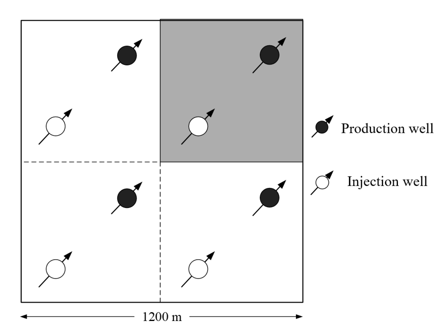
2.1. Physical Model and Boundary Conditions

In this study, we will conduct a numerical study on the thermal recovery performance of an idealized EGS model. The configuration of the injection and production wells utilized in the model is depicted in Figure 1. Due to the periodicity of the well distribution, a region with the length and width of 600 m, respectively, is selected, as shown in Figure 2. The region described by the physical model (see Figure 2) is 3500–5200 m underground, and the depth of the top and bottom surfaces of this physical model is 3500 m and 5200 m, respectively. The height of the fractured reservoir is 600 m, shown as the green region in Figure 2. Furthermore, considering that the surrounding strata may affect the numerical results, a cap region and a base rock with a height of 300 m and 800 m, respectively, are adopted. The depth of the injection well and production well are 4000 m and 4500 m, respectively.

The temperature and pressure in the hot dry rock reservoirs increase as the depth increases. The temperature and the pressure at 3500 m are 150 °C and 36 MPa, respectively, while these at 5200 m are 201 °C and 53 MPa, respectively. Due to the periodicity of this physical model, periodic boundary conditions are adopted for the sidewalls in Figure 2. For the heat transfer process, the top and bottom of this model are set as constant temperatures. For the mass transfer process, the top surface is set as constant pressure, and the bottom surface is set as an impermeable boundary. In addition, for the deformation process, the top and bottom of this model are set as constant normal stress. The temperature of the injected fluid is 25 °C, and the operating time of the system is assumed to be 30 years.

2.2. Governing Equations

In this study, the TOUGH2-EGS program is used for geothermal numerical simulations. TOUGH2 uses the integral finite difference method (IFDM) to discretize the spatial domain. Time is discretized fully and implicitly as a first-order backward finite difference. The general form of mass, energy, and geomechanics equations in the EGS reservoir can be given as [26]:

$$\frac{d}{dt}{{\displaystyle \underset{V_n}{\int }{M}^{k}d{V}_n={\displaystyle \underset{{\Gamma }_n}{\int }F}}}^k\cdot nd{\Gamma }_n+{\displaystyle \underset{V_n}{\int }{q}^{k}d{V}_n}$$

(1)

where k = 1, …, K is the number of the components; n = 1, …, N is the number of the grid; V_n represents the volume of the micro-unit. Γ_n is the boundary of the micro-unit, and n represents the normal vector of dΓ_n on the surface of the micro-unit; M^k denotes mass or energy for every unit volume; F^k represents mass or heat flow; q^k is the source item.

For the mass balance equation, M^k in Equation (1) can be expressed as [26]:

$${}^{M^k={\displaystyle \sum \varphi }{S}_{\beta }{\rho }_{\beta }{X}_{\beta }^{\kappa }}$$

(2)

where β = 1, …, N₀ represents the phase number of the component; $\varphi$ is the porosity; ρ_β and S_β are the density and the phase saturation of β phase, respectively; X_β^k represents the mass fraction of the k component in the β phase.

The mass flow in reservoirs can be calculated using the multi-phase Darcy law [26]:

$$F^k\left|{}_{adv}\right.={\displaystyle \sum _{\beta }{X}_{\beta }^{\kappa }}{F}_{\beta }$$

(3)

$$F_{\beta }=-k_0\left(1+\frac{b}{P_{\beta }}\right)\frac{k_{r\beta }{\rho }_{\beta }}{{\mu }_{\beta }}\left(\nabla P_{\beta }-{\rho }_{\beta }g\right)$$

(4)

where k₀ represents absolute permeability; k_rβ represents the relative permeability of β phase; μ_β and P_β are the dynamic viscosity and phase pressure of β, respectively; g represents the acceleration of gravity. b represents the gas slippage factor, if b = 0, it means the liquid phase;

For the energy equation, M^k in Equation (1) can be calculated with

$$M^k=(1-\varphi ){\rho }_R{C}_{R}T+\varphi {\displaystyle \sum _{\beta }{S}_{\beta }}{\rho }_{\beta }{u}_{\beta }$$

(5)

where C_R is the specific heat of the rocks, and ρ_R is the density of the rocks. T is the temperature, and u_β is the internal energy of β phase.

Heat transfer in EGS includes conduction, convection, and radiation heat transfer, and F^k in Equation (1) can be expressed as

$$F^k=-\left[\left(1-\varphi \right)K_R+\varphi {\displaystyle \sum _{\beta =1,2,3}{S}_{\beta }{K}_{\beta }}\right]\nabla T+f_{\sigma }{\sigma }_0\nabla T^4+{\displaystyle \sum _{\beta =1,2}{h}_{\beta }{F}_{\beta }}$$

(6)

where K_R indicates the thermal conductivity of rocks; f_σ is the surface radiation factor; h_β denotes the specific enthalpy of β phase; σ₀ indicates the Boltzmann constant.

This study assumes that the deformation of the boundary follows generalized Hooke’s law, and the equations of geomechanics can be expressed as [27]:

$$M^k=0$$

(7)

$$\frac{3(1-\nu )}{(1+\nu )}{\nabla }^2{\sigma }_m+\nabla \cdot \overline{F}-\frac{2(1-2\nu )}{(1+\nu )}(\alpha {\nabla }^{2}P+3EK{\nabla }^{2}T)=0$$

(8)

where E and α represent the linear thermal expansion coefficient and Biot coefficient, respectively. σ_m denotes the mean normal stress; K represents the bulk modulus; $\overline{F}$ and ν represents the body force and the Poisson’s ratio, respectively.

The hydraulic characteristics of EGS reservoirs, such as porosity, permeability, and capillary pressure, will change due to the influence of geomechanics. Therefore, when performing simulations on the flow and heat transfer in the reservoir, the dynamic changes in these parameters should be taken into account.

For stress-induced changes in porosity and permeability, Rutqvist et al. [28] presented the following function for porosity:

$$\varphi ={\varphi }_r+\left({\varphi }_0-{\varphi }_r\right)e^{-a{\sigma }^{\prime }}$$

(9)

where ${\varphi }_0$ is zero effective stress porosity, ${\varphi }_r$ is effective stress porosity, and $a$ is a parameter related to a specific rock. σ′ is the effective stress defined as [29]:

$${\sigma }^{\prime }=\sigma -\alpha P$$

(10)

where P is pressure, σ is the normal stress, and α is the Biot coefficient.

An associated correlation for permeability in terms of porosity also is given as [28]:

$$k=k_0{e}^{c(\frac{\varphi }{{\varphi }_0}-1)}$$

(11)

For the fracture network, Rutqvist et al. [28] defined the aperture width b_i in the direction i as function of effective stress:

$$b=b_{0,i}+\Delta b=b_{0,i}+b_{\max }({{\displaystyle e}}^{-d{\sigma }^{\prime }}{{\displaystyle -e}}^{-d\sigma 0^{\prime }})$$

(12)

where subscript 0 refers to initial conditions, ∆b is the aperture change, which is function of maximum “mechanical” aperture b_max, initial and current effective stress σ_0′ and σ′, and fracture specific parameter d. Fracture porosity is correlated to the aperture b as

$$\varphi ={\varphi }_0\frac{b_1+b_2+b_3}{b_{1,0}+b_{2,0}+b_{3,0}}$$

(13)

and permeability in direction i is correlated to fracture aperture of other directions j and k as

$$k_i=k_{i,0}\frac{{{\displaystyle b}}_j^3+{{\displaystyle b}}_k^3}{{{\displaystyle b}}_{j,0}^3+{{\displaystyle b}}_{k,0}^3}$$

(14)

The change in porosity and permeability will change the capillary pressure in the reservoir. The calculation formula for capillary pressure can be given as follows [30]:

$$P_c=P_{c0}\frac{\sqrt{{\left(k/\varphi \right)}_0}}{\sqrt{k/\varphi }}$$

(15)

2.3. Embedded Discrete Fracture Model

In the embedded discrete fracture model (EDFM), fracture and matrix grids are generated individually. The grids are then coupled to each other via source/sink relations. Due to this modeling method, EDFM is adaptable and simple to utilize. The connection between the matrices in the EDFM model is determined using the discretized version of the mass flux term [23].

$${\displaystyle {\int }_{{\Gamma }_n}{F}_{\beta }}\cdot nd{\Gamma }_n={\displaystyle \sum _{j\in {\eta }_i}{\left({\overline{\rho }}_{\beta }{\lambda }_{\beta }\right)}_{ij+1/2}^{n+1}}{\gamma }_{ij}\left[{\Phi }_{\beta j}^{n+1}-{\Phi }_{\beta j}^n\right]$$

(16)

$${\lambda }_{\beta }=\frac{k_{r\beta }}{{\mu }_{\beta }}$$

(17)

where η_i represents the adjacent elements directly connected to element i; Φ_βj represents the potential energy of beta in node j; λ_β is the transition rate.

The conductivity of the flow term is expressed as follows:

$${\gamma }_{ij}=\frac{A_{ij}{k}_{ij+1/2}}{d_i+d_j}$$

(18)

where A_ij represents the contact area between the fracture and the matrix; d_i denotes the average perpendicular distance from each point in the matrix grid to the fracture; d_j is the perpendicular distance from the fracture grid center point to the contact surface between the fracture and matrix; k_ij+1/2 represents the effective permeability. Pluimers et al. [31] provided analytical solutions for the values of d_i, d_j, and A_ij in the above equation.

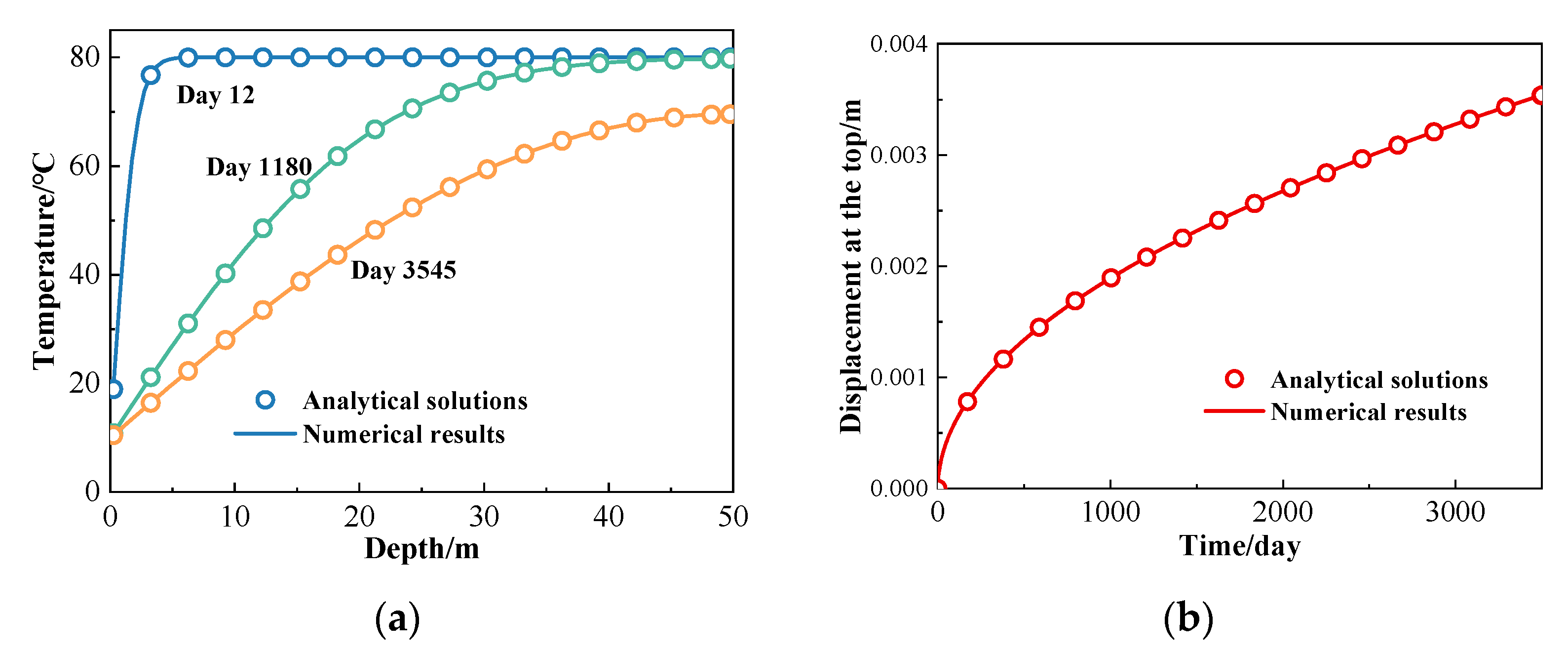
2.4. Method and Model Verification

To examine the accuracy of the simulation program, the heat conduction process in an impermeable rock column subjected to uniaxial strain in the vertical direction, as shown in Figure 3, is conducted. Initially, the temperature is 80 °C, then a lower temperature of 10 °C is applied on the top surface. When heat conduction occurs, there will be a displacement on the top surface of the column. Detailed parameters required for this case, including initial conditions and physical properties, are listed in

Table 1. Parameters for heat conduction problem [33].

Parameters	Value
Elastic modulus (GPa)	14.40
Poisson ratio	0.20
Porosity	0.01
Conductivity (W/m·K)	2.34
Heat capacity (J/kg·K)	690
Thermal expansion (K−1)	1.5 × 10−6
Initial mean stress (MPa)	3.0

. The analytical solutions of temperature distributions and displacement can be obtained using the finite Fourier transform [32]. Figure 4a,b shows the evolution of temperature with depth and the top surface deformation at different times, respectively. It indicates that the present numerical results are consistent with the analytical ones, which verifies the accuracy of the program and the numerical implementation.

The second test case is the heat transfer process in a single straight fracture (see Figure 5), in which the width of the fracture is 0.03 m, and the length of the matrix is 10 m. In addition, the rock matrixes are assumed to be homogeneous and isotropic and maintained at 80 °C. The water with a temperature of 30 °C and a flow rate 0.001 kg/s will transport across the fracture and absorb heat from the rock matrixes.

Table 2. Parameters used in the second test case.

Parameters	Value
Rock density (kg/m3)	14.40
Heat capacity (J/kg·K)	1000
Conductivity (W/m·K)	3.0
Matrix porosity	0.01
Fracture porosity	1.0
Matrix permeability (m2)	3.2 × 10−18
Fracture permeability (m2)	3.2 × 10−9

denotes the parameters used in this case.

Figure 6 compares the calculated temperature fields in the fracture with the analytical solutions [34]. The excellent consistency between present numerical results and analytical solutions in Figure 6 again proves the reliability of the program.

3. Results and Discussion

In this section, the evolution of pressure, temperature, effective stress, and porosity–permeability properties of the EGS embedded with fracture networks are firstly investigated using the THM coupling model. Then, the impact of some controllable factors, such as the fracture morphology, well distance, and injection rate, on EGS mining performance is analyzed and discussed.

3.1. Thermal-Hydraulic-Mechanical Characteristics of EGS with Fracture Networks

In order to investigate the thermal–hydraulic–mechanical characteristics of EGS using the THM coupling model, a physical model embedded with fracture networks is established, as shown in Figure 7. In this model, the total volume of fractures is 6656.25 m³, in which the vertical fractures and the horizontal fractures account for 55% and 45%, respectively. To explore the parameter variations at different locations in the reservoir, three locations a, b and c are taken as reference points, and the positions are shown in Figure 7b. The porosity and permeability of these cracks are 0.3 and 3.2 × 10⁻⁹ m², respectively. The width of fractures is 3 cm, and the other parameters of fractures are listed in

Table 3. Main parameters of the reservoir and fractures.

Parameters	Value	Parameters	Value
Rock density (kg/m3)	2600	Young’s module (GPa)	14.4
Heat capacity (J/kg·K)	1000	Poisson ratio	0.2
Thermal conductivity (W/m·K)	2.0	Coefficient of Biot	1
Matrix porosity	0.1	Linear thermal expansion (°C−1)	4.14 × 10−6
Fracture porosity	0.3	Productivity index	1.03 × 10−12
Matrix permeability (m2)	3.2 × 10−14	Water injection rate (kg/s)	8
Fracture permeability (m2)	3.2 × 10−9	Bottomhole production pressure (MPa)	33.25

. It should be noted that it is challenging to obtain the physical properties of the reservoir for actual geothermal fields. Therefore, the values of these parameters are chosen according to their ranges published in the available literature [24,35,36,37].

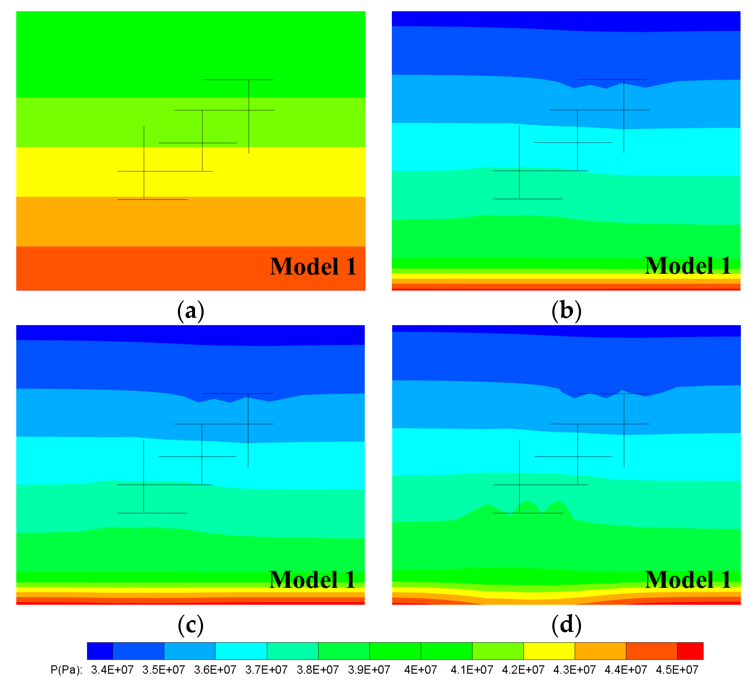
3.1.1. Evolution of Pressure Field

Figure 8 shows the evolution of the pressure in the reservoir. Figure 8 demonstrates that the pressure of the reservoir changes significantly in first five years.. This is because the pressure of the producing well is lower than the initial reservoir pressure, and the difference in pressure between the initial reservoir and the producing well causes the reservoir pressure to drop rapidly. Then, the stable pressure difference between the injection well and production well impels the reservoir pressure to reach equilibrium with a different temperature distribution. After that, there is no apparent change in the pressure field of the reservoir. This is because the pressure difference between the injection well and the producing well changes little within the production time. The slight differences in the pressure field at five years and 30 years are mainly attributed to the reservoir permeability change caused by the stress variation.

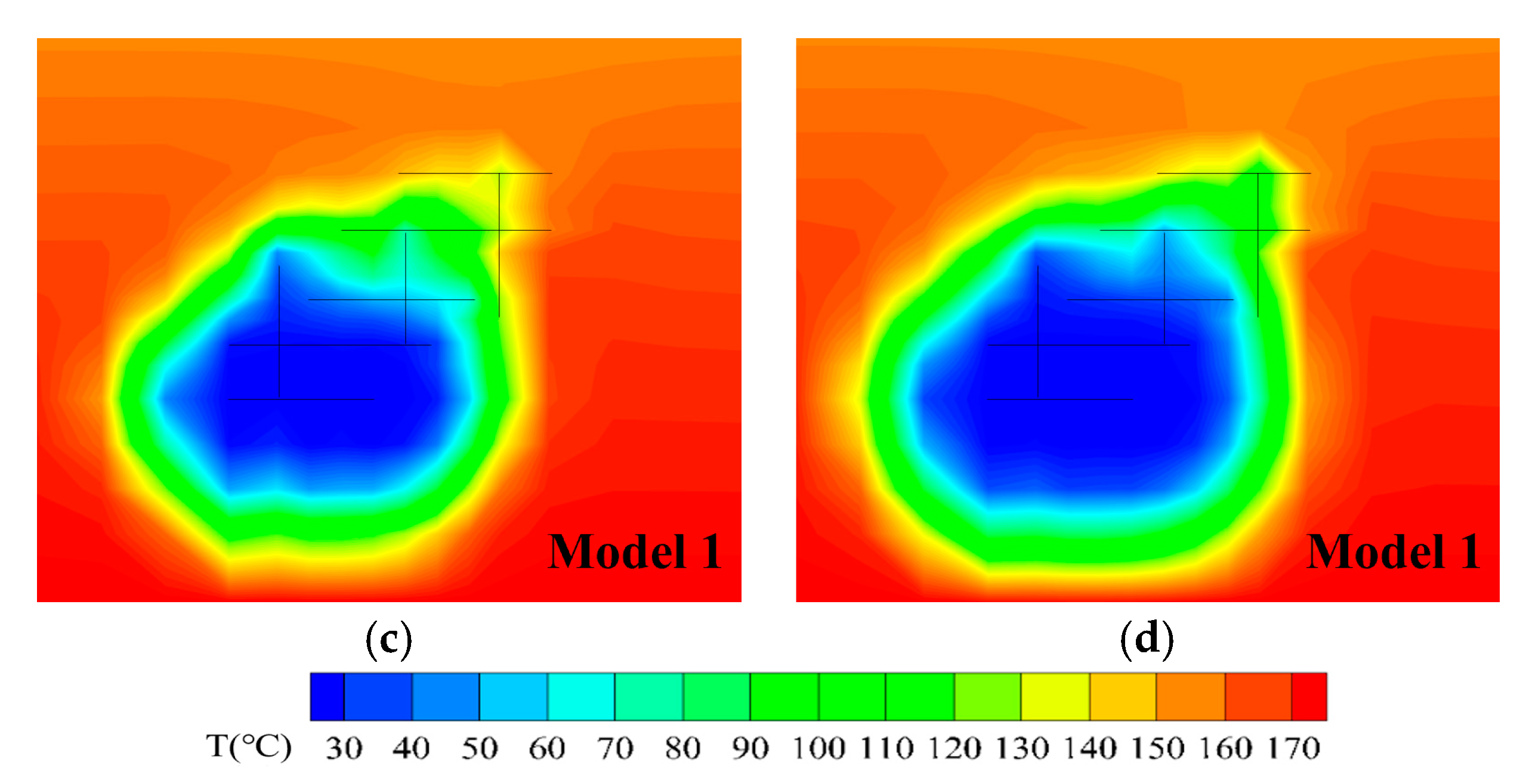
3.1.2. Evolution of Temperature Field

Figure 9 displays the temperature distribution of Model 1 at 5, 10, 20, and 30 years following operation. The results reveal that as time increases, the temperature near the injection well drops to the injection temperature of 25 °C rapidly, and then the low-temperature region gradually expands from the injection well to the production well. The low-temperature region mainly extends along the fracture networks, and the temperature change outside the fracture region is tiny. This phenomenon can be attributed to the fact that the cold working fluid predominantly flows through the fractures, which offer substantially lower flow resistance than the rocks.

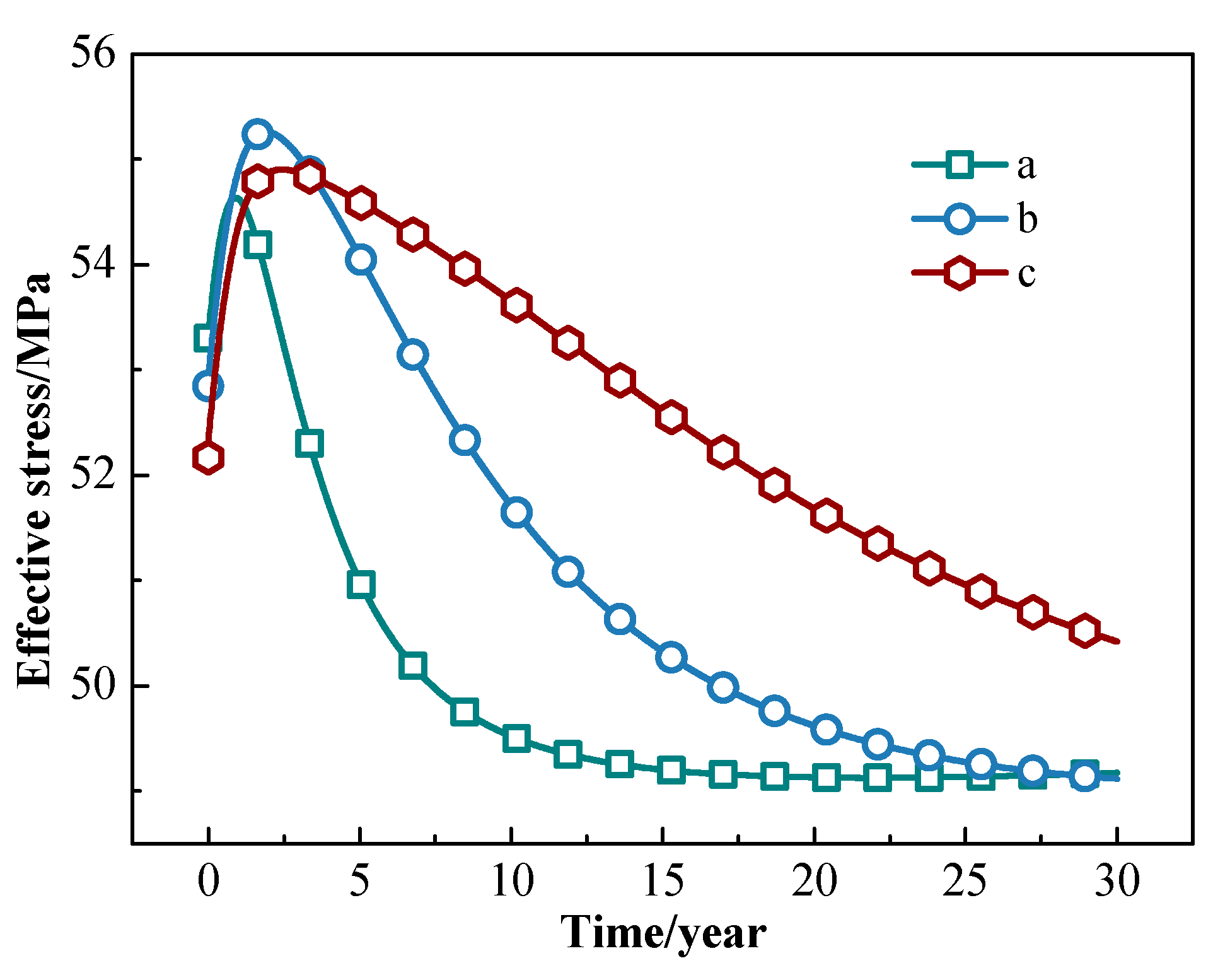
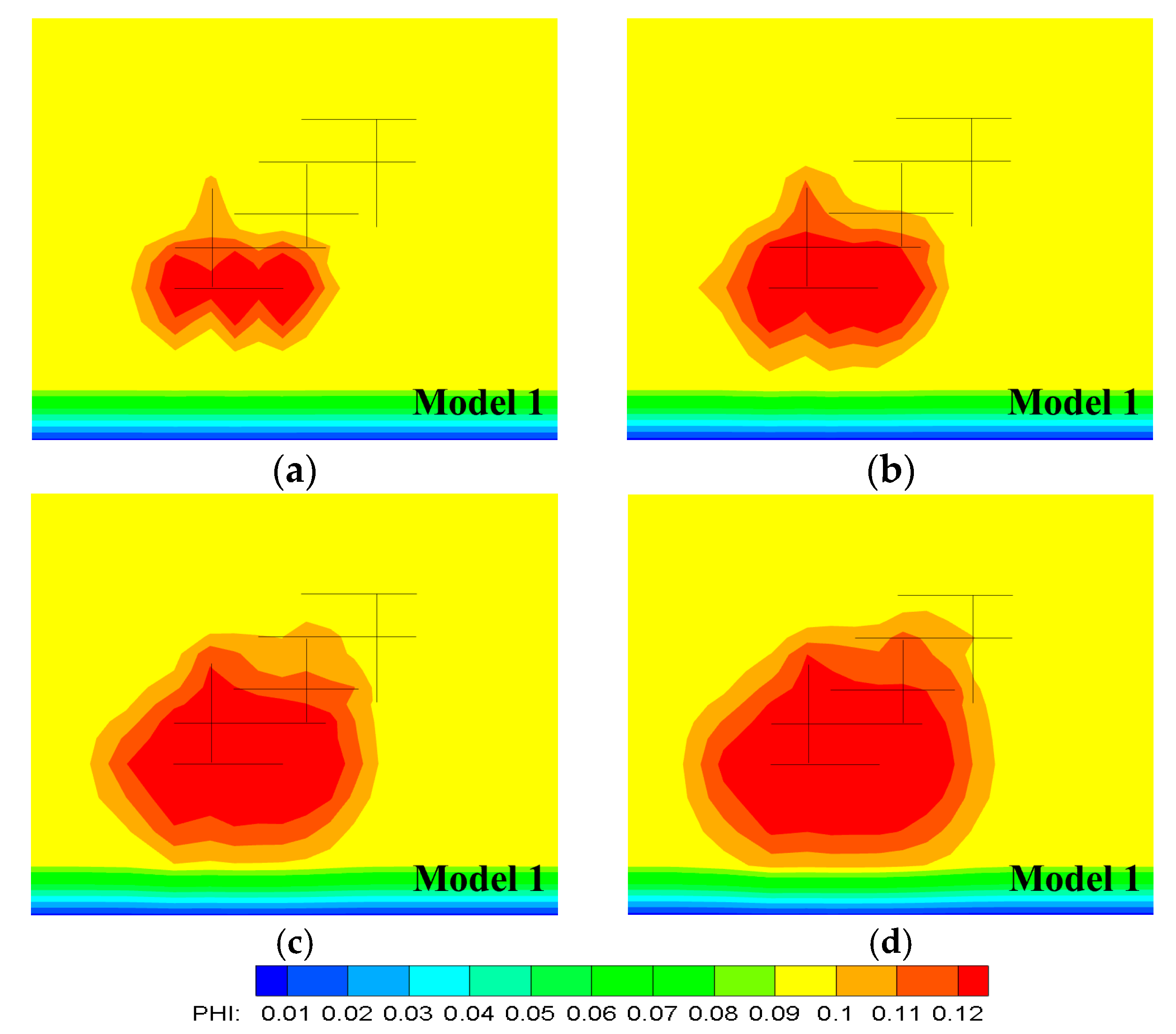
3.1.3. Evolution of Effective Stress Field

Figure 10 shows the evolution of the effective stress field of Model 1 at the mining time of 5, 10, 20, and 30. It is found that the injection of cold fluid results in the reduction in effective stress near the injection well. As time goes by, the low effective stress predominantly spreads along the fracture networks between the injection well and the production well, which is similar to the evolution of the temperature distribution. Figure 11 plots the local effective stress of points #a, #b, and #c (see Figure 7b) as a function of time. It indicates that the effective stress of these three locations increases at an early time and then decreases as time goes by. This phenomenon occurs because the pressure field propagation during the initial mining stage causes a rapid decline in pore pressure, which elevates the effective stress. Subsequently, the reservoir is cooled by the injection fluid, and the thermal stress comes to play a dominant role, thus leading to a decrease in the effective stress.

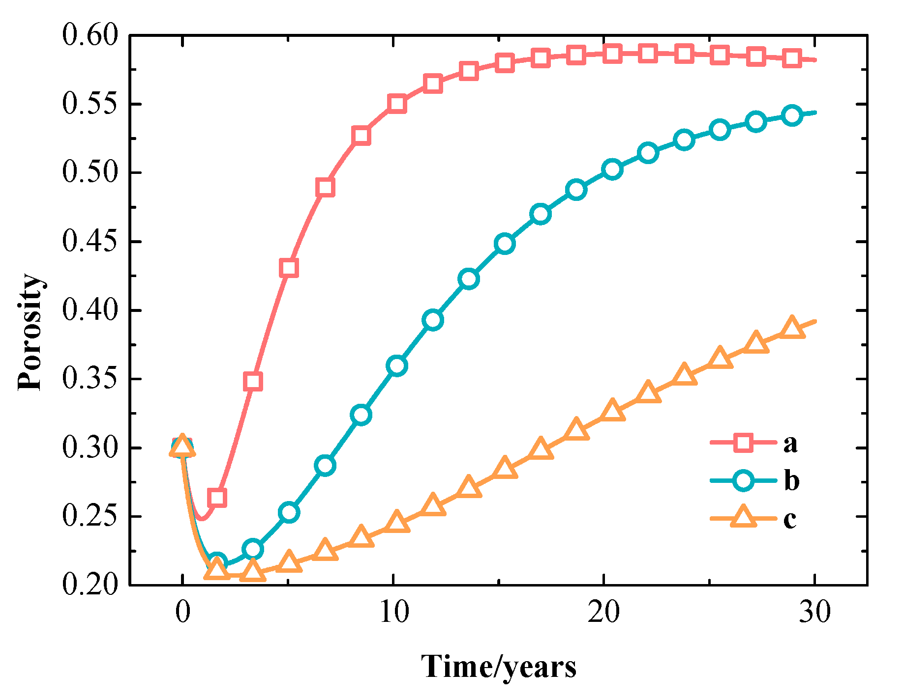
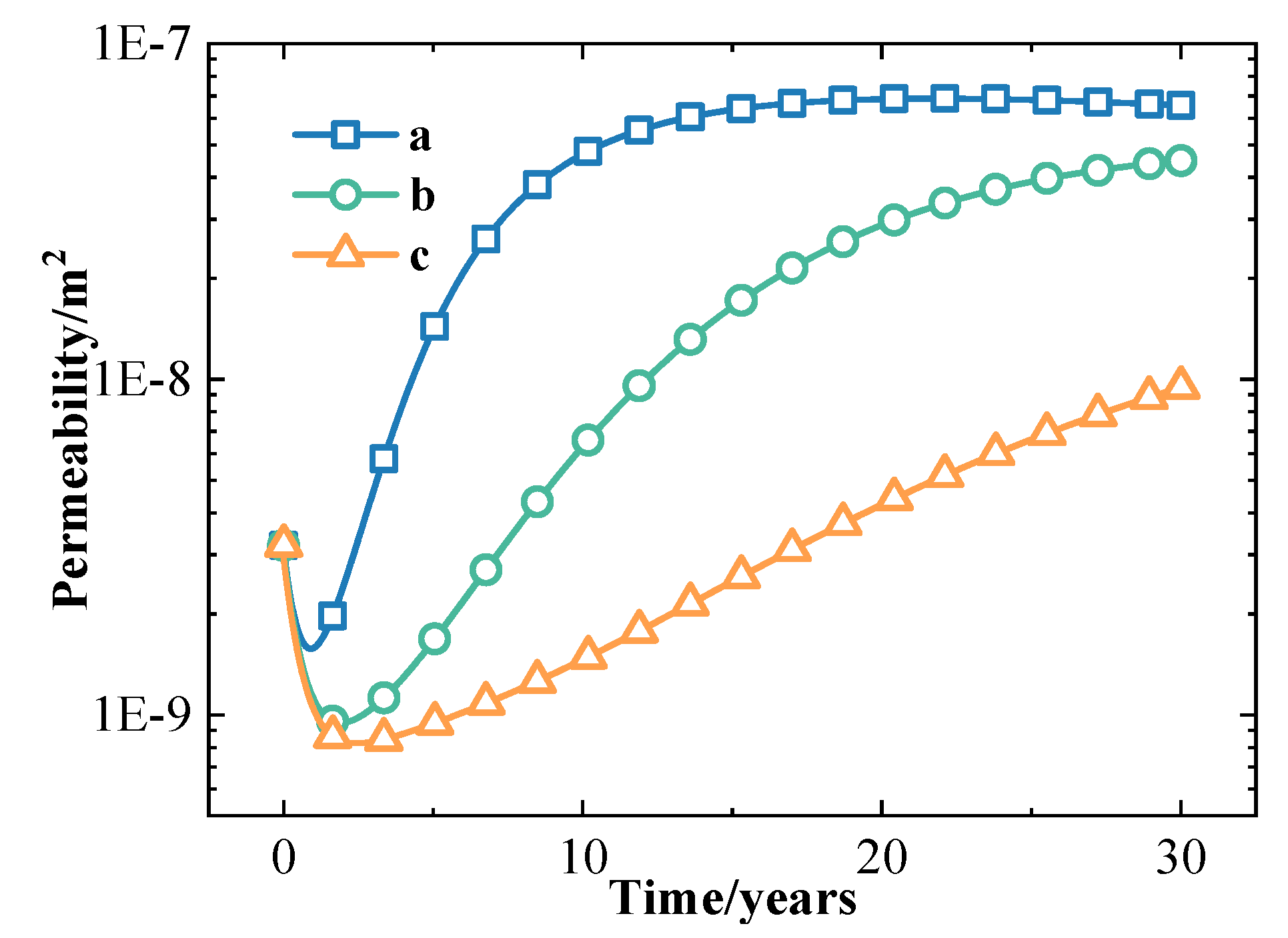
3.1.4. Evolution of Porosity and Permeability Properties

The change in the effective stress results in the change in reservoir porosity and permeability parameters. Figure 12 shows the evolutionary process of porosity at different times. It can be seen from Figure 10 and Figure 12 that the decrease in effective stress results in an increase in porosity.

Figure 13 and Figure 14 depict the changes in porosity and permeability, respectively, at specific locations (#a to #c) over time due to mining activities. The results of Figure 13 indicate that the porosity displays almost a contrary tendency with effective stress (see Figure 11), i.e., as time increases, the local porosities firstly decrease and then increase. Within the first two years of mining, the porosities of the three points (#a to #c) decrease from 0.3 to 0.248, 0.216, and 0.207, respectively, and then finally increase to 0.586, 0.543, and 0.391, respectively. In addition, it can be found that the porosity near the water injection well is larger. This is because the lower temperature around the injection well leads to lower effective stress. The evolution of local permeability shows similar trends of local porosity, i.e., as time increases, the local permeability firstly decreases and then increases.

3.2. Parametric Study of the Thermal Recovery Capacity

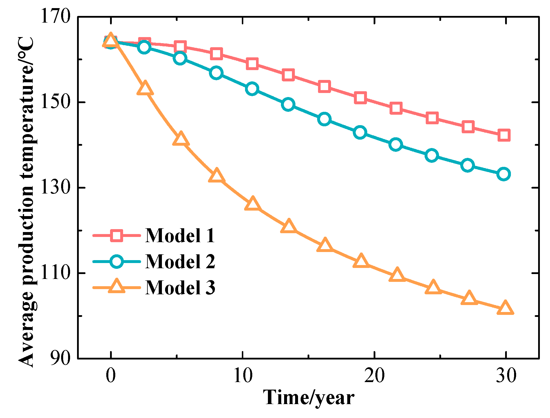
3.2.1. Effect of the Fracture Morphology

In order to investigate the impact of the fracture morphology, two different fracture networks are also established, as illustrated in Figure 15. The initial boundary condition of Model 2 and Model 3 is the same as Model 1 (See Figure 7a), and only the direction of the fractures is different. The comparison between the parameters of fractures in various models is listed in

Table 4. The parameters of different fracture networks.

Models	The Volume of the Total Fractures	The Fraction of Vertical Fractures	The Fraction of Horizontal Fractures	The Fraction of Inclined Fractures
Model 1	6656.25 m3	45%	55%	0.0%
Model 2	6712.50 m3	55%	45%	0.0%
Model 3	6434.61 m3	33.3%	33.3%	33.3%

. These three models have almost the same volume of total fractures, while the fracture morphology is different. In physical Model 1 (see Figure 7), there are no inclined fractures, and the horizontal fractures dominate in volume, accounting for 55%. In physical Model 2 (see Figure 15a), the horizontal fractures and vertical fractures account for 45% and 55%, respectively. In physical Model 3 (see Figure 15b), the vertical fractures, horizontal fractures, and inclined fractures each account for 1/3.

Figure 16 plots the average production temperature of the above models as a function of time. It can be seen that, as exploitation time increases, the average production temperature of Model 3 drops rapidly. At the 30th year after the operation of the EGS, the average production temperature in Model 3 decreases from 164 °C to 101.5 °C, and the average production temperature reduction is up to 38.1%. Correspondingly, the final average production temperatures in Model 2 and Model 1 are 133°C and 142 °C, respectively. Thus, at the 30th year after the operation of the EGS, Model 1 exhibits the best performance with the highest production temperatures. Moreover, it is observed that, unlike in Model 3, the production temperatures in Model 1 only change slightly within 10 years, indicating that Model 1 is relatively stable in a short time. This is because the vertical fractures and inclined fractures in Model 2 and Model 3 make it easier for cold fluid to flow directly between the injection and the production wells without performing sufficient heat exchange with the rock matrix. In contrast, the dominant horizontal fractures in Model 1 lead the cold fluid to move horizontally, thereby increasing the path for the heat exchange between flow and rocks, and consequently leading to a gradual rise in production temperatures.

To evaluate the heat recovery capacity, the heat recovery of the system is defined as follows:

$$W_{{}_h}=q(h_{pro}-h_{inj})$$

(19)

where h_pro indicates the specific enthalpy of the produced fluid, KJ/kg; h_inj is the specific enthalpy of the injected fluid with a temperature of 25 °C, and the corresponding specific enthalpy is about 146 KJ/kg; q denotes the flow rate of the produced fluid, kg/s.

Figure 17 shows the heat recovery of different models as a function of the exploitation time. It can be seen that, with the increase in the running time, the heat recovery of these three models decreases monotonously. At 30 years after the EGS has begun running, the reductions in heat recovery are 17.3%, 23.3%, and 46.6% for the different models, respectively.

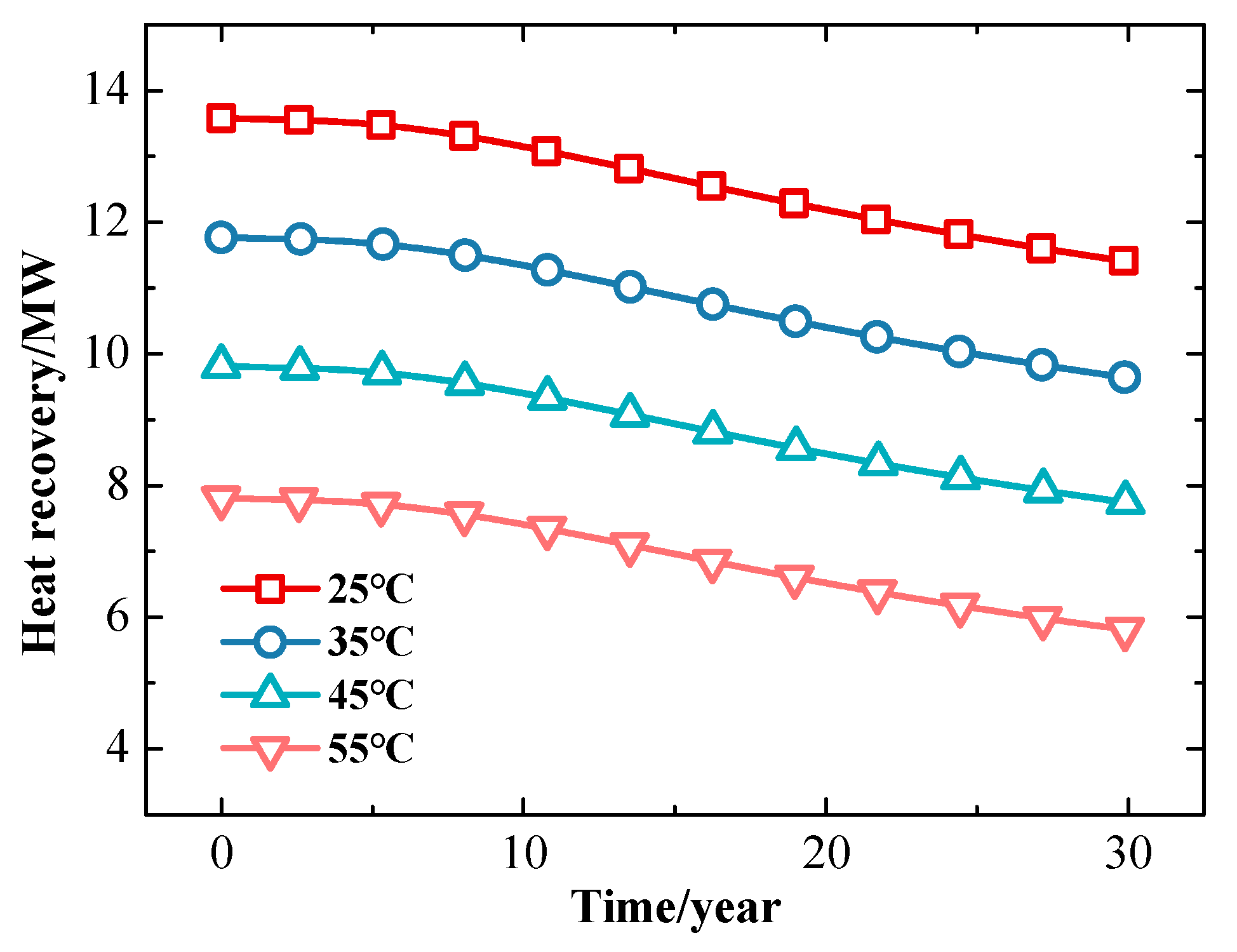
3.2.2. Effect of the Injection Temperature

Given that Model 1 demonstrated superior performance in Section 3.2.1, in the following section, we will mainly focus on the performance of Model 1. The injection temperatures of 25 °C, 35 °C, 45 °C, and 55 °C are selected to study the influence of the injection temperature and the thermal recovery potential of the EGS. The average production temperatures are plotted as a function of time in Figure 18. Notably, the production temperatures remain almost constant within the first 10 years of operation, regardless of the injection temperature. Subsequently, with the increase in injection temperature, the production temperature increases slightly. At 30 years after the operation, when the temperature of the injected fluid increases from 25 °C to 55 °C, the production temperature increases from 142.2 °C to 144.0 °C, with an increment of 1.2% only. This means the injection temperature barely influences the production temperature.

The heat recovery with different injection temperatures is shown in Figure 19. It is observed that, with the increase in the injection temperature, the heat recovery decreases. This outcome is attributed to the fact that decreasing the injection temperature enhances the temperature disparity between injection and extraction fluids, thereby increasing heat recovery. In the first 5 years, the heat recovery at different injection fluid temperatures is relatively stable, and the heat recovery with injection temperatures of 25 °C, 35 °C, 45 °C, and 55 °C is 13.5 MW, 11.7 MW, 9.7 MW, and 7.7 MW, respectively. Then, as time goes by, the heat recovery begins to decrease gradually. From 5 to 30 years, the heat recovery at the injection temperature of 25 °C gradually decreases from 13.5 MW to 11.4 MW. Thirty years after the operation, as the injection temperature increases from 25 °C to 55 °C, the heat recovery decreases from 11.4 MW to 5.8 MW, with a decrease of up to 49%. That means that reducing the injection temperature is an effective way to increase the heat recovery capacity.

3.2.3. The Effect of the Injection Flow Rates

To investigate the influence of injection flow rates on the heat recovery capacity, five different injection flow rates, i.e., 6.0, 7.0, 8.0, 9.0, and 10.0 kg/s, are selected. Figure 20 shows that the average production temperatures vary with time at different injection flow rates. It can be found from Figure 20 that the production temperatures with different injection rates in the first 3 years are almost 164 °C, which is relatively stable. Then, the value of the production temperature with different injection flow rates begins to decrease with the increase in operation time, and the production temperature decreases monotonically as the flow rate increases. At 30 years after the operation, the production temperatures with the flow rates of 6.0, 7.0, 8.0, 9.0, and 10.0 kg/s decrease from 164 °C to 149.8 °C, 145.8 °C, 142.2 °C, 138.7 °C and 135.5 °C, respectively.

Figure 21 shows the variation of the heat recovery with different injection flow rates. It indicates that the heat extraction of the system increases as the injection flow rate increases, but the growth rate decreases with the increase in the operation time. In addition, with the increase in time, the heat recovery with different injection flow rates decreases monotonically. This is because, as time goes by, the temperature of the rock decreases, resulting in reduced heat transfer between fluid and rock.

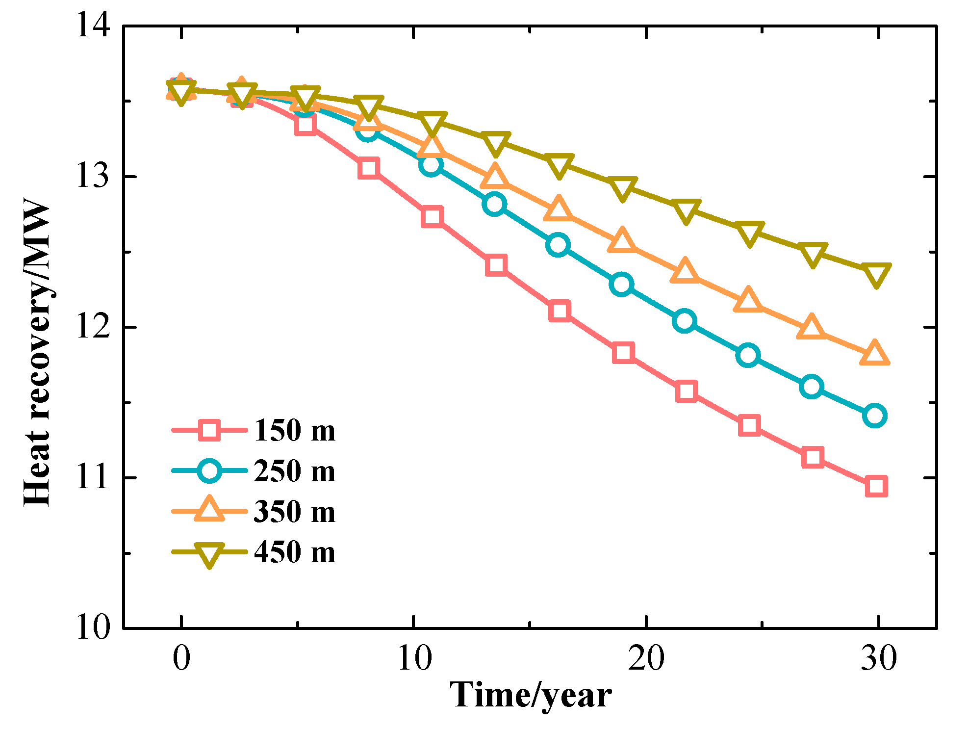
3.2.4. The Effect of the Injection–Production Well Spacing

In order to analyze the influence of the injection–production well spacing on heat extraction performance, four different cases with injection–production well spacing of 150 m, 250 m, 350 m, and 450 m are selected for simulations. Figure 22 plots the average production temperatures as a function of time for different well spacing. It can be seen from Figure 22 that, as the distance between the injection well and the production well increases, the production temperature increases, while the growth rate becomes gradually inconspicuous. When the distance between injection and production wells is 150 m, the production temperature begins to decrease after the system has been running for about 2 years, and the production temperature drops from 164 °C to 137.5 °C after 30 years. Correspondingly, the production temperature drops for the well spacing of 250 m, 350 m, and 450 m are 21.8 °C, 17.8 °C, and 12.2 °C, respectively, in 30 years. This can be attributed to the fact that, with the increase in the injection–production well spacing, the path that the working fluid travels becomes longer, and the working fluid can be continuously heated.

The heat recovery of EGS with different injection–production well intervals that varies with time is similar to the production temperature, as shown in Figure 23. It can be seen that, at the 30th year after mining, increasing the injection–production well spacing from 150 m to 450 m results in a heat production increase from 10.9 MW to 12.4 MW, representing a significant increase of 13.7%. Therefore, it is necessary to choose the well spacing appropriately for economic benefits and mining stability.

4. Conclusions

This paper presents numerical simulations to investigate the heat extraction performance and each physical field’s evolution of EGS by taking into account the THM coupling effect based on the EDFM model. The influences of fracture morphology, injection temperature, injection flow rates, and injection–production well intervals on the heat recovery temperature are examined. The key findings are as follows:

(1)

The fracture networks form the main flow channels in the reservoir. At the mining stage, the low temperature and the low mean effective stress caused by the low temperature in reservoirs extend mainly along the fracture networks between the injection well and the production well. The effective stress increases mainly under the influence of pore pressure at the initial stage of mining and decreases at the later stage due to the effect of thermal stress. As the mining time increases, the local porosity and permeability parameters first decrease and then increase.

(2)

In the present studied cases, the vertical fractures and inclined fractures are not conducive to geothermal exploitation because they could accelerate thermal breakthrough.

(3)

The production temperature is not sensitive to the injection temperature of the cold flow, while the heat recovery capacity drops dramatically with the increase in injection temperature.

(4)

Within the first 10 years of mining, the effect of the injection flow rates on the production temperature is insignificant. As time goes by, the production temperature decreases with the increase in injection flow rates. Because the heat recovery capacity is proportional to the flow rate, the heat recovery capacity in this study increases as the flow rate increases within 30 years.

(5)

Injection and production well spacing is one of the most critical factors that significantly influence the production temperature. In the test cases, the production temperature and heat recovery amount increase as the well spacing increases.

References

1. Chen, J.; Jiang, F. Designing multi-well layout for enhanced geothermal system to better exploit hot dry rock geothermal energy. Renew.. Energy 2015, 74, 37–48. [Google Scholar] [CrossRef]
2. Salimzadeh, S.; Nick, H.M.; Zimmerman, R.W. Thermoporoelastic effects during heat extraction from low-permeability reservoirs. Energy 2018, 142, 546–558. [Google Scholar] [CrossRef]
3. Wei, X.; Feng, Z.; Zhao, Y. Numerical simulation of thermo hydro-mechanical coupling effect in mining fault-mode hot dry rock geothermal energy. Renew. Energy 2019, 139, 120–135. [Google Scholar] [CrossRef]
4. Olasolo, P.; Juárez, M.C.; Morales, M.P.; Damico, S.; Liarte, I.A. Enhanced geothermal systems (EGS): A review. Renew. Sustain. Energy Rev. 2016, 56, 133–144. [Google Scholar] [CrossRef]
5. Leontidis, V.; Niknam, P.H.; Durgut, I.; Talluri, L.; Manfrida, G.; Fiaschi, D.; Akin, S.; Gainville, M. Modelling reinjection of two-phase non-condensable gases and water in geothermal wells. Appl. Therm. Eng. 2023, 223, 120018. [Google Scholar] [CrossRef]
6. Niknam, P.H.; Talluri, L.; Fiaschi, D.; Manfrida, G. Sensitivity analysis and dynamic modelling of the reinjection process in a binary cycle geothermal power plant of Larderello area. Energy 2021, 214, 118869. [Google Scholar] [CrossRef]
7. Zhang, J.; Xie, J.X. Effect of reservoir’s permeability and porosity on the performance of cellular development model for enhanced geothermal system. Renew. Energy 2020, 148, 824–838. [Google Scholar] [CrossRef]
8. Schoenball, M.; Dorbath, L.; Gaucher, E.; Wellmann, F.; Kohl, T. Change of stress regime during geothermal reservoir stimulation. Geophys. Res. Lett. 2014, 41, 1163–1170. [Google Scholar] [CrossRef]
9. Egert, R.; Nitschke, F.; Gholami Korzani, M.; Kohl, T. Stochastic 3D Navier-Stokes Flow in Self-Affine Fracture Geometries Controlled by Anisotropy and Channeling. Geophys. Res. Lett. 2021, 48, e2020GL092138. [Google Scholar] [CrossRef]
10. Marchand, S.; Mersch, O.; Selzer, M.; Nitschke, F.; Schoenball, M.; Schmittbuhl, J.; Nestler, B.; Kohl, T. A Stochastic Study of Flow Anisotropy and Channelling in Open Rough Fractures. Rock Mech. Rock Eng. 2019, 53, 233–249. [Google Scholar] [CrossRef]
11. Jiang, F.; Chen, J.; Huang, W.; Luo, L. A three-dimensional transient model for EGS subsurface thermo-hydraulic process. Energy 2014, 72, 300–310. [Google Scholar] [CrossRef]
12. Luo, F.; Xu, R.N.; Jiang, P.X. Numerical investigation of fluid flow and heat transfer in a doublet enhanced geothermal system with CO2 as the working fluid (CO2-EGS). Energy 2014, 64, 307–322. [Google Scholar] [CrossRef]
13. Aliyu, M.D.; Chen, H.P. Enhanced geothermal system modelling with multiple pore media: Thermo-hydraulic coupled processes. Energy 2018, 165, 931–948. [Google Scholar] [CrossRef]
14. Yin, T.; Li, Q.; Hu, Y.; Yu, S.; Liang, G. Coupled thermo-hydro-mechanical analysis of valley narrowing deformation of high arch dam: A case study of the xiluodu project in China. Appl. Sci. 2020, 10, 524. [Google Scholar] [CrossRef]
15. Vik, S.H.; Salimzadeh, S.; Nick, H.M. Heat recovery from multiple-fracture enhanced geothermal systems: The effect of thermoelastic fracture interactions. Renew. Energy 2018, 121, 606–622. [Google Scholar] [CrossRef]
16. Yao, J.; Zhang, X.; Sun, Z.; Huang, Z.; Liu, J.; Li, Y.; Xin, Y.; Yan, X.; Liu, W. Numerical simulation of the heat extraction in 3D-EGS with thermal-hydraulic-mechanical coupling method based on discrete fractures model. Geothermics 2018, 74, 19–34. [Google Scholar] [CrossRef]
17. Sun, Z.-X.; Zhang, X.; Xu, Y.; Yao, J.; Wang, H.-X.; Lv, S.; Huang, Y.; Cai, M.-Y.; Huang, X. Numerical simulation of the heat extraction in EGS with thermal-hydraulic-mechanical coupling method based on discrete fractures model. Energy 2017, 120, 20–33. [Google Scholar] [CrossRef]
18. Gan, Q.; Elsworth, D. Production optimization in fractured geothermal reservoirs by coupled discrete fracture network modeling. Geothermics 2016, 62, 131–142. [Google Scholar] [CrossRef]
19. Shi, Y.; Song, X.; Li, J.; Wang, G.; Zheng, R.; YuLong, F. Numerical investigation on heat extraction performance of a multilateral-well enhanced geothermal system with a discrete fracture network. Fuel 2019, 244, 207–226. [Google Scholar] [CrossRef]
20. Lee, S.H.; Jensen, C.L.; Lough, M.F. An efficient finite difference model for flow in a reservoir with multiple length-scale fractures. SPE J. 2000, 5, 268–275. [Google Scholar] [CrossRef]
21. Lee, S.H.; Lough, M.F.; Jensen, C.L. Hierarchical modeling of flow in naturally fractured formations with multiple length scales. Water Resour. Res. 2001, 37, 443–455. [Google Scholar] [CrossRef]
22. Praditia, T.; Helmig, R.; Hajibeygi, H. Multiscale formulation for coupled flow-heat equations arising from single-phase flow in fractured geothermal reservoirs. Comput. Geosci. 2018, 22, 1305–1322. [Google Scholar] [CrossRef]
23. Wang, C.; Winterfeld, P.; Johnston, B.; Wu, Y.S. An embedded 3D fracture modeling approach for simulating fracture-dominated fluid flow and heat transfer in geothermal reservoirs. Geothermics 2020, 86, 101831. [Google Scholar] [CrossRef]
24. Li, T.; Han, D.; Yang, F.; Li, J.; Wang, D.; Yu, B.; Wei, J. Modeling study of the thermal-hydraulic-mechanical coupling process for EGS based on the framework of EDFM and XFEM. Geothermics 2020, 89, 101953. [Google Scholar] [CrossRef]
25. Yu, S.; Song, X.J.; Feng, Y.J. Effects of lateral-well geometries on multilateral-well EGS performance based on a thermal-hydraulic-mechanical coupling model. Geothermics 2021, 89, 101939. [Google Scholar]
26. Pruess, K.; Oldenburg, C.; Moridis, G. TOUGH2 User’s Guide Version 2; Office of Scientific & Technical Information Technical Reports; University of California: Berkeley, CA, USA, 1999. [Google Scholar]
27. Huang, X.; Zhu, J.; Li, J.; Lan, C.; Jin, X. Parametric study of an enhanced geothermal system based on thermo-hydro-mechanical modeling of a prospective site in Songliao Basin. Appl. Therm. Eng. 2016, 105, 1–7. [Google Scholar] [CrossRef]
28. Rutqvist, J.; Wu, Y.S.; Tsang, C.F. A Modeling Approach for Analysis of Coupled Multiphase Fluid Flow, Heat Transfer, and Deformation in Fractured Porous Rock. Int. J. Rock Mech. Min. Sci. 2002, 39, 429–442. [Google Scholar] [CrossRef]
29. Biot, M.A.; Willis, D.G. The Elastic Coefficients of the Theory of Consolidation. J. Appl. Mech. 1957, 24, 594–601. [Google Scholar] [CrossRef]
30. Leverett, M.C. Capillary behavior in porous media. AIME Trans. 1941, 142, 341–358. [Google Scholar] [CrossRef]
31. Pluimers, S.B. Hierarchical Fracture Modeling Approach. Master’s thesis, TU Delft, Delft University of Technology, Delft, The Netherlands, 2015. [Google Scholar]
32. Bai, B. One-dimensional thermal consolidation characteristics of geotechnical media under non-isothermal condition. Eng. Mech. 2005, 22, 186–191. [Google Scholar]
33. Fakcharoenphol, P.; Xiong, Y.; Hu, L.; Winterfeld, P.H.; Xu, T.; Wu, Y.S. User’s Guide of TOUGH2-EGS: A Coupled Geomechanical and Reactive Geochemical Simulator for Fluid and Heat Flow in Enhanced Geothermal Systems. Version 1.0; Petroleum Engineering Department of Colorado School of Mines: Golden, CO, USA, 2013. [Google Scholar]
34. Barends, F.B.J. Complete solution for transient heat transport in porous media, following Lauwerier’s concept. Proc. SPE Annu. Tech. Conf. Exhib. 2010, 4, 3139–3150. [Google Scholar]
35. Shi, Y.; Song, X.; Wang, G.; Li, J.; Geng, L.; Li, X. Numerical study on heat extraction performance of a multilateral-well enhanced geothermal system considering complex hydraulic and natural fractures. Renew. Energy 2019, 141, 950–963. [Google Scholar] [CrossRef]
36. Yan, X.; Huang, Z.; Yao, J.; Li, Y.; Fan, D. An efficient embedded discrete fracture model based on mimetic finite difference method. J. Pet. Sci. Eng. 2016, 145, 11–21. [Google Scholar] [CrossRef]
37. Guo, L.; Zhang, Y.; Yu, Z.; Hu, Z.; Lan, C.; Xu, T. Hot dry rock geothermal potential of the Xujiaweizi area in Songliao Basin, northeastern China. Environ. Earth Sci. 2016, 75, 1–22. [Google Scholar] [CrossRef]
Figure 1. The arrangement of injection–production wells.
Energies 16 03758 g001
Figure 2. Reservoir model and well arrangements.
Energies 16 03758 g002
Figure 3. One-dimensional heat conduction in a deformable rock column.
Energies 16 03758 g003
Figure 4. Comparison between present results and analytical solutions: (a) temperature curve; (b) top displacement curve.
Energies 16 03758 g004
Figure 5. A single fracture heat transfer model.
Energies 16 03758 g005
Figure 6. Temperature distribution in the fracture at different times.
Energies 16 03758 g006
Figure 7. Physical model of fractured reservoir: (a) 3D physical model; (b) distribution of injection and production wells.
Energies 16 03758 g007
Figure 8. Pressure field distributions of the EGS at different times: (a) 0 years, (b) 5 years, (c) 10 years, and (d) 30 years.
Energies 16 03758 g008
Figure 9. Temperature field distributions of the EGS at different times: (a) 5 years, (b) 10 years, (c) 20 years, and (d) 30 years.
Energies 16 03758 g009aEnergies 16 03758 g009b
Figure 10. Evolution of effective stress field: (a) 5 years, (b) 10 years, (c) 20 years, and (d) 30 years.
Energies 16 03758 g010
Figure 11. Evolution of local effective stress as a function of extraction time.
Energies 16 03758 g011
Figure 12. Evolution of porosity field: (a) 5 years, (b) 10 years, (c) 20 years, and (d) 30 years.
Energies 16 03758 g012
Figure 13. Evolution of porosity of points #a to #c with extraction time.
Energies 16 03758 g013
Figure 14. Evolution of permeability of different locations with extraction time.
Energies 16 03758 g014
Figure 15. Physical models of reservoirs with different fracture networks: (a) Model 2 and (b) Model 3.
Energies 16 03758 g015
Figure 16. Average production temperature of EGS with different fracture morphologies.
Energies 16 03758 g016
Figure 17. Evolution of the heat production power of different models with time.
Energies 16 03758 g017
Figure 18. Influence of the injection temperature on the production temperature.
Energies 16 03758 g018
Figure 19. The influence of the injection temperature on heat recovery.
Energies 16 03758 g019
Figure 20. Effect of the injection flow rates on the production temperature.
Energies 16 03758 g020
Figure 21. The influence of injection flow rates on heat recovery.
Energies 16 03758 g021
Figure 22. The influence of the injection–production well spacing on the production temperature.
Energies 16 03758 g022
Figure 23. The influence of the injection–production well spacing on heat recovery.
Energies 16 03758 g023