Leading Point Multi-Regression Model for Detection of Anomalous Days in German Energy System

Abstract

In this article, the Leading Point Multi-Regression model was applied to identify days with anomalous energy consumption profiles. The data for the analysis come from the German energy system and they represent the hourly energy demand observed between 2006 and 2015. Days with abnormal daily profiles were identified based on the statistical analysis of the errors observed for the model. The accuracy of the model is very high and comparable with other models, e.g., LSTM, K-means, Recurrent NN, and tree-based ML methods. However, these methods rely on external factors (e.g., humidity, temperature, and sunshine) impacting energy consumption while our model uses only the energy consumption at specific fixed hours, regardless of external factors, thus being universal. Days with anomalous energy consumption profiles were identified as days related to celebration of New Year’s Eve and the New Year. Also, anomalies were identified for some other days, which were not that obvious, including Good Friday, National Day of Mourning, and, interestingly, the day of the Germany–Turkey match during the European Championship in 2008.

1. Introduction

The energy market has undergone a revolution in recent years. A new group of consumers emerged who do not only buy energy but also produce it [1]. Moreover, in recent years, when the prices of energy went up, some new challenges for intelligent energy management appeared [2]. The interest in new renewable sources of energy is growing. On the other hand, techniques of energy consumption optimization became more crucial. Simple methods of predicting energy demand became insufficient [3]. In recent years, a couple of new methods for demand analysis have been proposed. They go beyond classical methods such as Holt-Winters or ARIMA [4]. More advanced machine learning (ML) and nonlinear methods have been often utilized in order to forecast power demand more accurately. For instance, RF (random forest) [5], ANNs (artificial neural networks) [6], K-Nearest Neighbors (KNNs) [7], support vector machines (SVMs) [7,8], and gradient boosting machine (GBM) [9] are quite commonly applied for energy modeling. The analysis of energy consumption focused on identification of the energy demand sources and other external factors which influence consumption became very important, including weather conditions, season, holiday periods, and economics [5]. In context of proper energy management, the event-triggered methods, hybrid policy-based reinforcement learning, dual sequence prediction models (DSPMs), and technology acceptance models are new streams that have been analyzed recently [10,11,12,13].

Another important aspect of the energy consumption analysis is peak identification and anomaly detection. In [14], the authors deal with these issues using artificial neural networks. That technique is further extended with CART (Classification and Regression Trees) and the KNN classifier. In other work [6], generalized combined additive models and deep ANN are used to identify high-resolution peak loads. Another important issue in the modeling of power demand is the identification of outliers [15]. They are commonly described as time periods with an unusual consumption of energy. The problem is especially important from the tuning point of view of power systems and energy price optimization. Outlier detection was performed using the hybrid model as a combination of Long Short-Term Memory (LSTM) and the K-means algorithm [16]. The LSTM is the most commonly used variety of Recurrent Neural Networks (RNNs). The combination of the deep learning model and K-means clustering approach was utilized to model energy consumption over time and to detect various anomalies [17]. The authors showed that the method used outperformed the most commonly used LSTM model for the time series. In [18], the ensemble tree-based ML method, i.e., RF and GBM, was adopted to mitigate overfitting and to deal with unbalanced data. Another unsupervised ML method of outlier detection was used in [19].

In this paper, we analyze hourly energy consumption data from the German power system for the period between 2006 and 2015. Specifically, we focus on identifying days with unusual energy consumption profiles. For that purpose, we use the Leading Points Multi-Regression model (LPMR) [20] that describes hourly energy consumption for the entire day using only a few automatically identified hours, which are key for the model. By days with unusual profiles, we mean those that the model describes with a high error.

The practical value of anomaly detection in electricity consumption is significant as it is one of the key important activities to ensure a system’s reliability. The knowledge about expected anomalies helps to maintain a balance between electricity production and consumption and to maintain the quality and continuity of services for the customers.

As provided in [17,21], the majority of works are focused on identification of peak demands using historical load data, weather variables, calendar variables, and, sometimes, macroeconomic variables. The novelty of our work is that, in contrast to the other studies, with LPMR, we do not focus on peak detection only but we go beyond this because we are interested in anomaly detection which occurs when the model does not describe the daily profile with sufficiently high precision. Therefore, with the LPMR model, we are able to identify abnormal days (which may be the peak days or days with low consumption) with no upfront assumptions and no preliminary selection of such days. Also, as far as input data are concerned, the LPMR model is not dependent on any external data like weather or calendar variables, thus being universal.

The precision of the model is very high, regardless of other external factors like season, weather conditions, or calendar variables. In order to identify outliers with the model, we used the error measures and defined the ranges for these errors. Taking into account the values of the errors, we detected days with unusual daily energy consumption profiles, verified them, and investigated their characteristics. This way, we can draw conclusions about the reasons for the untypical profiles.

This paper is organized as follows. Section 2 presents the data set used for the analysis. This is followed by the model methodology outlined in Section 3. Section 4 presents the model estimation followed by the analysis of anomalous daily profiles in Section 5. Section 6 summarizes key insights from the study and presents areas for future work.

2. Data Characteristics

This study focuses on the data regarding total electricity consumption in the German energy system [22]. The electricity usage in MWh was observed on an hourly basis. The data covered a time span between 1 January 2006 and 31 December 2015. The authors carefully reviewed the data to be sure that it covered whole days with no gaps. The data being analyzed contained 3642 days, which corresponded to 87,408 h. While our model uses energy consumption data solely, some additional variables were used for the purpose of discussing the results, in particular, to distinguish specific days and associated hours, such as weekdays, specific holidays days, working hours, etc.

For data analysis, the data set was split into the training and the testing sample (50% each). The data sets contain 1821 days for training and another 1821 days for testing. All of the results were based on the testing set, to avoid self-correlations. On the other hand, we dealt with some periodicities. The main periodicity was related to the daily energy consumption profile, which was the main subject of our studies. They are presented in Figure 1a for the period of 2 weeks. In addition, the data revealed the weekly and yearly periodicities. They are visible in Figure 1b,c. However, we show further in the paper that the model used was immune to those periodicities.

The whole data set was divided into 24 time series, each with hourly electricity usage. Further, 24 variables were prepared: $E\left(h_m\right)=\left(E_1\left(h_m\right), \dots , E_i\left(h_m\right), \dots , E_N\left(h_m\right)\right)$, where $h_m\in \left\{h_1, h_2, \dots , h_{24}\right\}$, $E_i\left(h_m\right)$ is the electricity consumption at hour $h_m$ on the i-th day, and N is the total number of days.

3. Leading Points Multi-Regression Model

3.1. The Model Formula

The model used in this paper was presented and discussed in detail in [20]. Its main purpose is to model hourly energy consumptions for the whole day, with only a few variables being used. The independent variables were energy consumption at certain hours. The model itself detects the set of leading hours based on the presumed precision. However, in this research, we use the model to detect anomalous days from the energy consumption perspective.

The multiple equation linear regression model is used to describe energy consumption and it is as follows:

$$E\left(h_p\right)=a_{0p}+a_{1p}E\left(h_1\right)+a_{2p}E\left(h_2\right)+\cdots +a_{kp}E\left(h_k\right)+{\xi }_p$$

(1)

where $p\in \left\{1, \dots , 24\right\}\setminus \left\{1, \dots , k\right\}$ and $a_{0p}, a_{1p}, \dots , a_{kp}$ are the model parameters. The number of equations in the final model is related to the number of features used. In the case of k variables, the model consists of 24 − k equations.

Model (1) uses electricity consumptions at certain hours $h_1, h_2, \dots , h_k$ and with them, it describes electricity usage for the remaining hours. The variable selection process of the model is based on the properties of the random components ${\xi }_p$. For each equation in the model, a standard deviation of the residuals is calculated. The formula depends on the number of independent variables k in the model and has the following form:

$$\sigma \left(h_p\right)=\sqrt{\frac{1}{N-k-1}{{\displaystyle \sum }}_{i=1}^N{\left(E_i\left(h_p\right)-{\widehat{E}}_i\left(h_p\right)\right)}^2}$$

(2)

where ${\widehat{E}}_i\left(h_p\right)$ denotes theoretical value and $E_i\left(h_p\right)-{\widehat{E}}_i\left(h_p\right)={\xi }_p$. The quality of the model regressions is also measured with the relative standard deviation:

$$\nu \left(h_p\right)=\sqrt{\frac{1}{N-k-1}{{\displaystyle \sum }}_{i=1}^N{\left(E_i\left(h_p\right)-{\widehat{E}}_i\left(h_p\right)\right)}^2}/\overline{E\left(h_p\right)}$$

(3)

where the standard deviation of residuals is divided by the mean of electricity consumption. The quality of the whole of Model (1) is measured with the mean values of Measures (4), i.e., mean standard deviation (MSD), and (5), i.e., mean relative standard deviation (MRSD), which are calculated for all 24 − k equations in the model:

$$MSD=\frac{1}{24-k}{\displaystyle \sum }_{p=1}^{24-k}\sigma \left(h_p\right),$$

(4)

$$MRSD=\frac{1}{24-k}{\displaystyle \sum }_{p=1}^{24-k}\nu \left(h_p\right).$$

(5)

3.2. The Algorithm for Variables’ Selection

The variables in the model are selected by the algorithm in the following steps. Starting with one independent variable, the model is expanded by changing the label of the variable from described to describing. The steps are repeated until the desired accuracy of the model is reached.

The first step: Twenty-four models with one independent variable are estimated. Each model consists of 23 equations, and the mean relative error MRSD is calculated. The algorithm chooses the best model—the one with the lowest MRSD. This is the first selected model and its describing variable $E\left(h_1\right)$ is the first selected independent variable.

During steps 2 to 23, a choice of the independent variable is performed based on another rule.

The second step: A mean squared error $\sigma \left(h_p\right)$ is calculated for each equation of the model chosen in the previous step. The algorithm chooses the worst described variable $E\left(h_2\right)$—the variable with the biggest error. This variable becomes the second independent variable. Then, the model with two independent variables $E\left(h_1\right)$ and $E\left(h_2\right)$ consisting of 22 equations is evaluated.

The third step and beyond: All the equations of the previous model are analyzed and the described variable with the maximum error $\sigma \left(h_p\right)$ is chosen. That variable becomes another independent variable of the model.

In each step, the mean errors MSD and MRSD are calculated. They allow for the evaluation of the precisions of the obtained models. In paper [20], we have proven that the procedure of variable selection described above leads to the best possible models. Each of the equations constructed is statistically significant.

4. Model Estimation

The models were evaluated using the training sample, n = 1821 days. In the first step, the algorithm analyzes 23 equations. The obtained values of MRSD error are shown in Figure 2a. The smallest value MRSD_min = 0.0480 corresponds to the hour $h_1=$ 16 and $E\left(h_1\right)$ became the first describing variable. In the next five steps, the algorithm selected $E\left(h_i\right)$ variables that described the following hours: $h_2=$ 2, $h_3=$ 24, $h_4=$ 7, $h_5=$ 18, and $h_6=$ 20. The changes in the MRSD error values in the successive steps are shown in Figure 2b and listed in

Table 1. The hours selected by the model based on the training data set.

Step	Hour	# Variables	# Equations	# Parameters	MRSD
1	$h_1=16$	1	23	46	0.0914
2	$h_2=2$	2	22	66	0.0463
3	$h_3=24$	3	21	84	0.0378
4	$h_4=7$	4	20	100	0.0341
5	$h_5=18$	5	19	114	0.0292
6	$h_6=20$	6	18	126	0.0198

. The procedure was stopped at step 6, because the error decreased below 2% and could be considered as acceptable. Although including more variables would help to reduce error further, being aware of parsimony principle, we prefer a model with fewer parameters over a more complex one when both models fit the data similarly well as there are multiple practical recommendations for this [23,24].

The MRSD error decreases with the number of independent variables. We observe a strong decrease in the error in steps 1–6. Just after step two, the relative error decreased below 5%; after step four, it was below 3.5%; and after step six, it reached a value below 2%. Subsequent error decreases are not so significant. On the other hand, one should keep in mind that the following models have a larger number of independent variables while describing a smaller number of hours. We concluded that six variables are sufficient to describe the data with reasonable accuracy. The chosen model contains six independent variables and 18 equations. The model evaluated on the training set has a mean absolute error equal to 799.06 MWh and a mean relative error equal to 1.26%, as shown in

Table 2. Model’s results in terms of MSD and MRSD.

Sample	MSD (In MWh)	MRSD
Training	799.06	0.0126
Testing	721.81	0.0117

.

The model was also verified on a testing data set. The quality was evaluated for each hour and for each day. For days, the quality of the model was evaluated using absolute and relative measures. The measures for the final model, which consists of 18 equations, are defined in line with the following formulas:

$$SD\left(i\right)=\sqrt{\frac{1}{18}{\displaystyle \sum }_{p=7}^{24}{\left(E_i\left(h_p\right)-{\widehat{E}}_i\left(h_p\right)\right)}^2}$$

(6)

$$RSD\left(i\right)=\sqrt{\frac{1}{18}{\displaystyle \sum }_{p=7}^{24}{\left(E_i\left(h_p\right)-{\widehat{E}}_i\left(h_p\right)\right)}^2}/\frac{1}{18}{\displaystyle \sum }_{p=7}^{24}{E}_i\left(h_p\right)$$

(7)

where, in the sum part, the following hours are omitted: from $h_1$ to $h_6$; i = 1, 2, …, N, and N represents the number of analyzed days. Measures (6) and (7) correspond to Measures (2) and (3), but the summary is calculated for hours instead of days.

The average values of SD and RSD errors on the testing data set are equal to 721.81 MWh and 1.17%, respectively, as shown in Table 2. On the testing set, they turned out to be even lower than those obtained on the training set. The model shows a very good fit since, for about 95% of days, the relative error does not exceed 2%. The daily total energy consumption is also described with high accuracy, as shown in Figure 3. The left part of Figure 3, i.e., Figure 3a, shows that the daily total energy predicted by the model fits well to the daily total empirical energy consumption. These predicted and empirical values were divided by one another to see the distribution, as shown in Figure 3b. The shape is perfectly Gaussian with a low standard deviation equal to 0.53% which indicates a very good fit. This indicates that for 99.8% of data, the model prediction is within 1.58% of the real data.

In this place, it is worth mentioning that the quality of the presented model is very high and comparable with other models, e.g., LSTM, K-means, Recurrent NN, and tree-based ML methods. The listed methods focus on the effects of external factors, humidity, temperature, sunshine, etc., on energy consumption. In turn, autoregressive models focus on the determination of energy consumption based on past energy consumption. Our model uses only energy consumption at specific fixed hours, regardless of external factors. For comparison, the regression tree algorithm [4] describes 96.6% of data with an error below 2% but it uses 18 describing variables. In paper [17], three models were discussed, LSTM, Transformer, and K-means, which have an accuracy between 96% and 97%, while our model represents the accuracy exceeding 98%. Moreover, artificial neural networks [14] represent an accuracy of about 96.2%. The novelty of this approach is that it allows us to model energy consumptions for the entire day using only a few selected hours. It also provides very accurate results regardless of external factors. One should emphasize that other models use a number of various factors influencing the energy consumption which are not always known with sufficient precision, and their errors propagate to the accuracy of the model. Moreover, in the case of nationwide systems, it is impossible to precisely take into account some factors such as temperature, humidity, etc., due to their variability both in space and time.

To illustrate the model’s performance, six randomly selected days were presented in Figure 4 to show empirical and theoretical time series. The values of SD and RSD errors for the presented days are provided in

Table 3. Selected days from the data set and daily absolute and relative model’s errors.

No	Date	Weekday	SD	RSD
1	8 December 2009	Monday	378.8	0.0054
2	22 May 2009	Thursday	820.0	0.0171
3	28 October 2011	Sunday	1006.8	0.0143
4	17 December 2011	Tuesday	409.4	0.0066
5	28 March 2014	Sunday	677.5	0.0108
6	21 November 2015	Thursday	575.4	0.0102

.

As shown in Figure 4, daily profiles show a very good fit of the model to the data. Theoretical time series reproduce the actual energy consumption with high accuracy; however, for some hours, a slight gap between empirical and theoretical values is noticeable. Specifically, $h=$ 19, 21 were difficult to capture accurately. Nevertheless, the aggregated data in Figure 4d show that each hour is described very well by the model.

5. Detection of Anomalous Daily Profiles

5.1. Analysis of the Errors

At first, the daily errors of the model were analyzed using plots. In Figure 5, the daily errors, i.e., absolute SD and relative RSD, of the model are shown for the whole data set. We observe that values of the errors do not exhibit any trend over time, so their values do not depend on the distance from the training data set.

The distributions of both errors are lognormal. The comparison between the distribution of errors’ logarithms with the normal distribution is shown in Figure 6. Specifically, Figure 6a,b present a Gaussian curve fitted to the data. For better presentation of the tails, the plots have a vertical log scale. The parameters of the normal distributions are listed in

Table 4. Estimates of the normal distribution parameters μ and σ fitted to logarithms of errors.

Variable	μ	σ	R2
log(SD)	6.582 ± 0.014	0.487 ± 0.007	0.991
log(RSD)	−4.476 ± 0.005	0.541 ± 0.008	0.990

. The Q-Q plots in Figure 6c,d demonstrate the agreement of theoretical and empirical distributions.

The distributions of log errors exhibit good fit with a normal distribution. However, there are visible deviations at the far ends of both tails. The number of counts is higher than for the theoretical distribution in those regions. Days in the left tail are characterized by a very good precision of the model used.

On the other hand, the right tail contains days for which the model has the greatest errors. Those days are anomalous, characterized by their abnormal daily profiles of energy usage. Further, the deviations from the normal distribution may suggest that some additional factors influencing the data can be present, apart from statistical fluctuations.

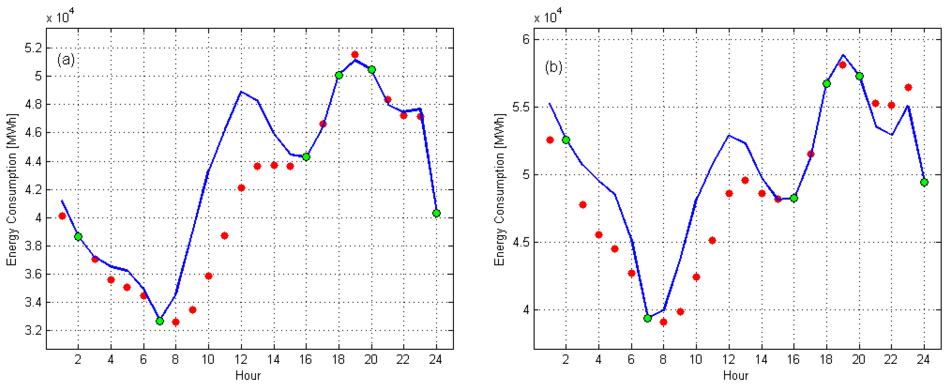
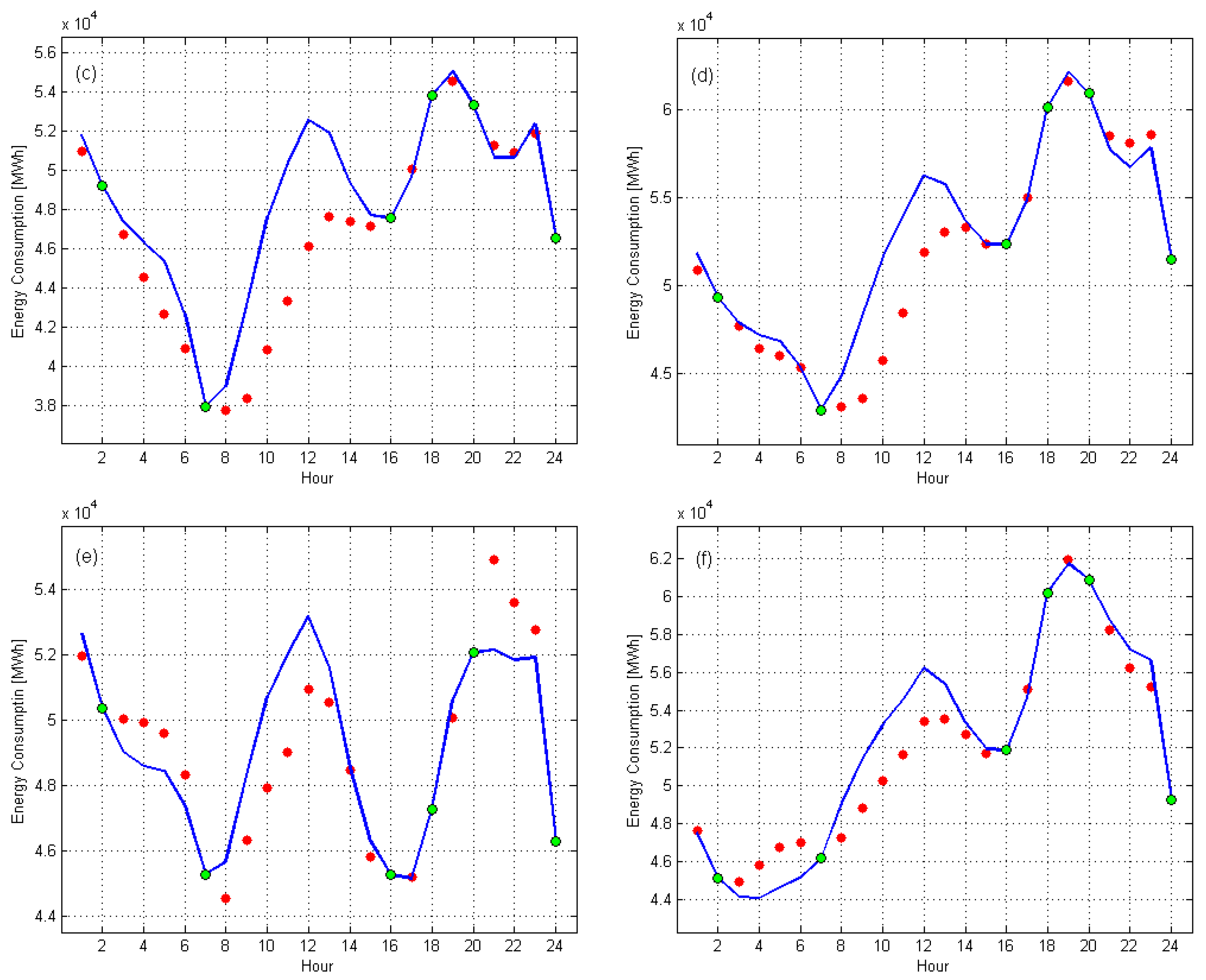
5.2. Identification of Anomalous Daily Energy Consumption Profiles

Based on the distribution of RSD, two threshold ranges of relative errors were considered as those which indicate anomalous energy consumption:

(1)

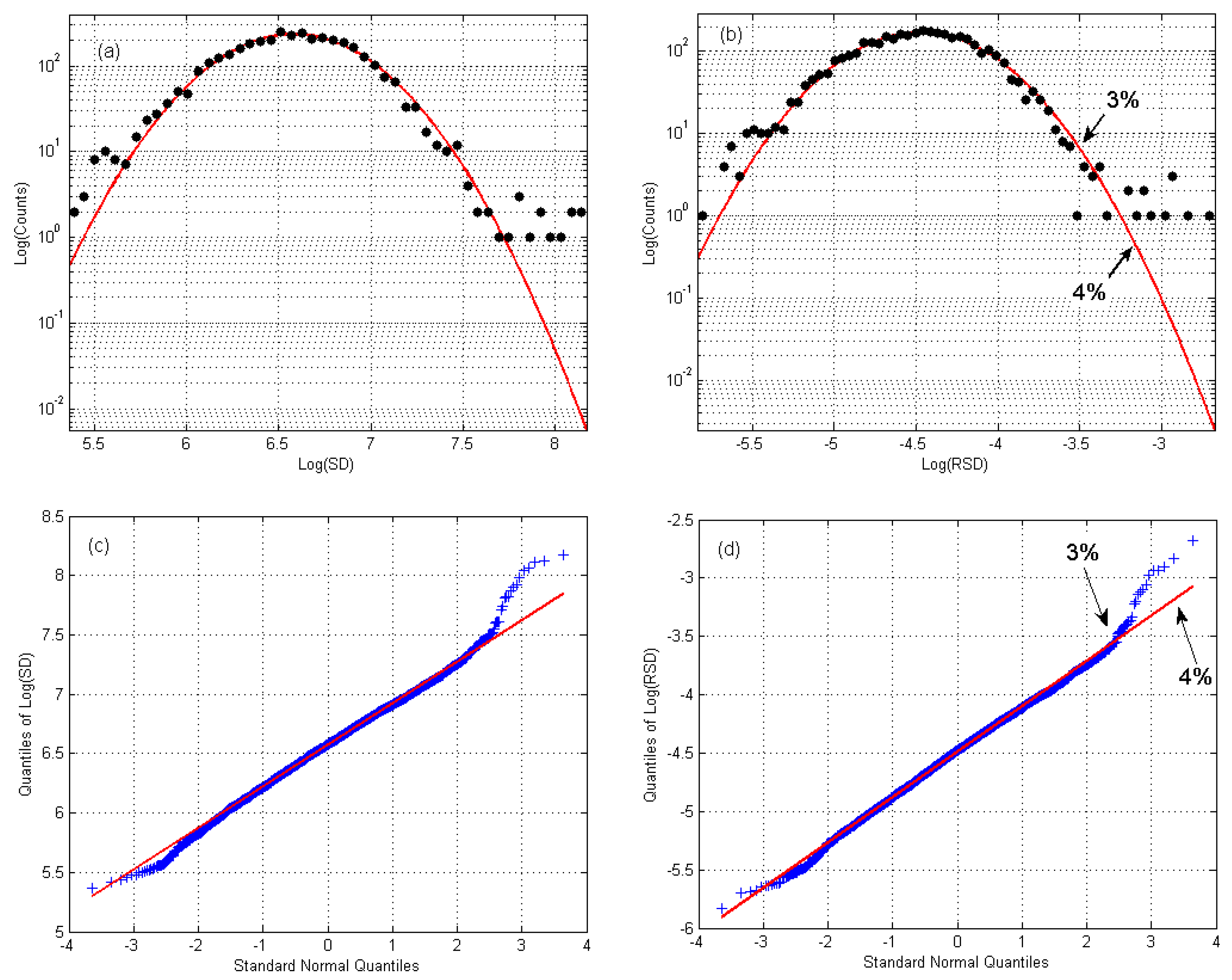
0.04 ≤ RSD (−3.22 ≤ log(RSD));

(2)

0.03 < RSD < 0.04 (−3.51 < log(RSD) < −3.22).

The boundaries between the thresholds are indicated by arrows in Figure 6b,d. We observe deviations from the normal distributions in both ranges. However, in the first range, the normal distribution is negligible, while in the second range, we may expect some days to be distributed according to the Gaussian curve. All the anomalous days from both ranges are listed in

Table 5. Anomalous days identified by the model. The data in the table are arranged by descending RSD. Weekdays start from 1 (Monday) till 7 (Sunday).

No	Date	RSD	Weekday	Description
1	1 January 2013	0.0685	2	New Year
2	1 January 2012	0.0591	7	New Year
3	1 January 2009	0.0547	4	New Year
4	1 January 2010	0.0532	5	New Year
5	1 January 2008	0.0531	2	New Year
6	1 January 2006	0.0508	7	New Year
7	1 January 2014	0.0469	3	New Year
8	1 January 2011	0.0453	6	New Year
9	1 January 2007	0.0442	1	New Year
10	31 December 2013	0.0431	2	New Year’s Eve
11	31 December 2012	0.0405	1	New Year’s Eve
12	1 January 2015	0.0400	4	New Year
13	19 March 2011	0.0357	6	Other
14	10 June 2011	0.0344	5	Other
15	31 December 2015	0.0343	4	New Year’s Eve
16	22 August 2010	0.0336	7	Other
17	16 May 2010	0.0335	7	Other
18	3 April 2010	0.0333	6	Holy Saturday
19	2 April 2010	0.0329	5	Good Friday
20	14 November 2010	0.0323	7	National Day of Mourning
21	31 December 2009	0.0315	4	New Year’s Eve
22	13 July 2014	0.0314	5	Other
23	22 March 2010	0.0313	1	Other
24	25 June 2008	0.0310	3	Germany vs. Turkey match during European Championship
25	28 October 2012	0.0303	7	Daylight Saving Time ends

.

There are 12 days in the first range that contain the days with the greatest errors—equal and above 0.04. The second group contains 13 days with errors greater than 0.03 and less than 0.04. All the anomalous days in the first group are related to the New Year (10 days) and New Year’s Eve (2 days), while the anomalous days identified in the second group are much more diverse. Specifically, we observe that New Year’s Eve days are captured, as are a couple of other days that are connected to catholic holidays—Holy Saturday and Good Friday. Also identified as anomalous were the National Day of Mourning, the day when the Germany–Turkey match took place during the European Championship 2008, the Daylight Saving Time ending day in 2008, and six other days that are not connected to any type of holiday or special events. These days do not appear systematically every year. They occurred as anomalous days only in the given year, while for the remaining years, these were just typical days, well described by the model (with low errors).

Next, the daily energy consumption data were plotted against daily RSD values as presented in Figure 7. It was conducted to analyze the specifics of energy consumption for anomalous days. It was observed that the majority of anomalous days (i.e., 22 out of 25) are characterized by low energy consumption, which is typical for holiday periods and non-working days.

In the following step, a deep dive analysis of the daily empirical and theoretical profiles for six anomalous days from Table 4 was performed, and it is presented in Figure 8.

It can be observed that the profiles of anomalous days significantly differ from the typical profiles shown in Figure 4. Regardless of the year, the New Year days have very similar profiles, as shown in Figure 8a–d. For these days, the model clearly overestimates the data between 8 a.m. and 4 p.m. The very unusual profiles are observed for Good Friday in Figure 8e and for the National Day of Mourning in Figure 8f. For these two days, the model overestimates the data during the day while underestimating it at night and early in the morning.

5.3. Discussion of the Results

Anomaly detection in electricity consumption data is a critical element in managing and enhancing the reliability of power systems. Often, the key issue is the definition of an untypical daily energy consumption profile. In this work, we follow a common approach, stating that it is a profile that is not well described by the model, i.e., a profile with high error. However, there is still an open question about how to determine the threshold of the error, as it may be dependent on the data specifics, country specifics, or the specific needs of the user.

In our study, we defined the errors’ thresholds precisely. On one hand, as an untypical day, we consider a day with a sufficiently high error value and, on the other hand, we assume that those days are the days where the error distribution deviates from its theoretical distribution (normal distribution for logarithms of errors).

Based on the distribution of RSD, we have considered two thresholds of the error: 0.04 (quantile 0.997) and 0.03 (quantile 0.993). Untypical profiles have high errors because of non-statistical reasons. They deviate from the Gaussian distribution of log-errors.

The days in the upper threshold range have model errors for which the theoretical distribution is negligible. Thus, for all the days in this range, daily profiles of energy consumption are untypical and caused by uncommon factors. In the second threshold range, untypical days are present, but we can also expect some days with regular profiles but with high errors.

At this moment, it is worth mentioning a similar study [25] that was prepared for the Polish data as the results can be compared with the results obtained on German data presented in this paper. Interestingly, there are differences observed between these two studies in terms of the model structure, i.e., the number of variables in the model, and in terms of the anomalous days identified by the model. Specifically, the model applied to Polish data used four variables (hour = 2, 14, 18, 20) with an RSD error equal to 0.0175 on the testing data. The model applied to German data uses six variables (hour = 2, 7, 14, 18, 20, 24) with an RSD error equal to 0.0117, while the same four variables are used in both models.

Also, a significant difference was observed for the days that were identified as anomalous. The analysis of Polish data has identified untypical days related to the biggest religious holidays: Easter, All Saints, and Christmas Eve. The first two are paid holidays, and the last one, if non-weekend, is a working day, but the working hours are usually shortened. The main factor causing anomalies in the daily profiles was related to the short-term migration of people. Finally, New Year’s Eve was identified as atypical for Polish data, too.

As far as the analysis of German data is concerned, mainly the New Year and New Year’s Eve were identified as anomalous. There were few examples of atypical days captured that were connected to catholic holidays—Holy Saturday and Good Friday. Finally, days identified as anomalous were the National Day of Mourning, the day when Germany–Turkey match took place during the European Championship in 2008, and the Daylight Saving Time end day in 2008.

It was quite surprising that we did not observe any anomalies in the daily profiles for other religious holidays celebrated in Germany, i.e., Easter Sunday and Monday, Corpus Christi, and Assumption Day, which are non-working days. Also, we did not observe any anomalies for other important public holidays, e.g., Labor Day and the Day of German Unity.

6. Conclusions

In this paper, the method applicable to the identification of days with anomalous daily profiles in terms of energy consumption was presented. The method was based on the Leading Points Multi-Regression model. The analysis utilized hourly energy consumption data in the German power system over the period of 10 years. The following conclusions can be drawn from the study:

• The novelty of LPMR is that it allows for modeling energy consumptions for the entire day using only a few selected hours.
• It has been shown that the energy consumption data can be modeled with high precision using six independent variables denoting energy consumption for the following hours: $h_1=$ 16, $h_2=$ 2, $h_3=$ 24, $h_4=$ 7, $h_5=$ 18, and $h_6=$ 20.
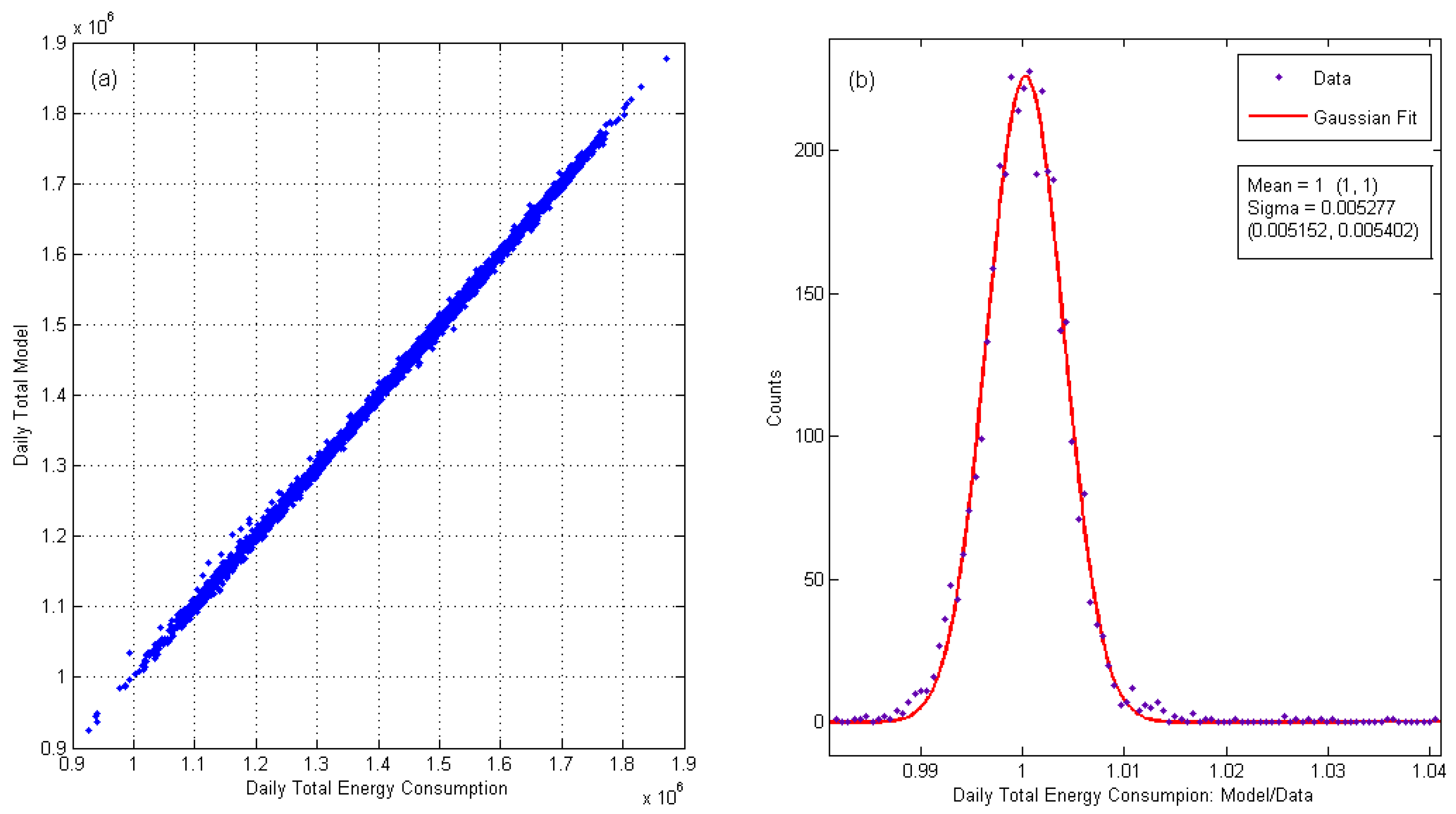
• The distribution of the model’s errors follows a Gaussian distribution with high accuracy.
• The anomalous days, with regard to energy consumption profiles, were accurately defined as these with high errors and falling into the range where the distribution deviates from Gaussian.
• Days with untypical profiles were mainly New Year and New Year’s Eve which was quite expected. However, there were a few other days that were considered atypical which were not so obvious. These were Holy Saturday and Good Friday which are connected to Catholic holidays. Also, other anomalous days were identified: National Day of Mourning, day when the Germany–Turkey match took place during the European Championship 2008, Daylight Saving Time end day in 2008, and six other days that are not connected to any type of holiday or special events.
• Anomalies in daily profiles were not observed in the case of other religious holidays as well as major public holidays, even when they fell on long weekends.
• It was observed that the majority of anomalous days were characterized by low energy consumption typical for holiday periods and non-working days.

The analysis presented in this paper can be easily extended to other countries and regions. We believe that anomaly detection is of great interest from a national perspective since unexpected events which impact energy consumption predictions often cause non-optimal energy production and create instability in the system.

As far as future research is considered, a focus on the distinction between low- and high-consumption anomalous days might be a promising direction from a system management and market balancing perspective. Specifically, the research question would be whether separate LPMR models are needed to detect low- and high-consumption anomalous days. Also, fitting the model in case of stationarity or in case there is a lack of stationarity observed in the data might potentially deliver conclusions for specific model use.

References

1. Sulich, A.; Sołoducho-Pelc, L. Changes in Energy Sector Strategies: A Literature Review. Energies 2022, 15, 7068. [Google Scholar] [CrossRef]
2. Marinakis, V.; Koutsellis, T.; Nikas, A.; Doukas, H. AI and Data Democratisation for Intelligent Energy Management. Energies 2021, 14, 4341. [Google Scholar] [CrossRef]
3. Chicco, G.; Mazza, A. Load profiling revisited: Prosumer profiling for local energy markets. In Local Electricity Markets; Pinto, T., Vale, Z., Winder-grean, S., Eds.; Academic Press: Cambridge, MA, USA, 2021; pp. 215–242. [Google Scholar]
4. Karpio, K.; Łukasiewicz, P.; Nafkha, R. Regression Technique for Electricity Load Modeling and Outlined Data Points Explanation. In Advances in Soft and Hard Computing; Peja’s, J., El Fray, I., Hyla, T., Kacprzyk, J., Eds.; Advances in Intelligent Systems and Computing; Springer: Cham, Switzerland, 2019; Volume 889, pp. 56–67. [Google Scholar]
5. Hong, T.; Fan, S. Probabilistic electric load forecasting: A tutorial review. Int. J. Forecast. 2016, 32, 914–938. [Google Scholar] [CrossRef]
6. Berrisch, J.; Narajewski, M.; Ziel, F. High-resolution peak demand estimation using generalized additive models and deep neural networks. Energy AI 2023, 13, 100236. [Google Scholar] [CrossRef]
7. Parhizkar, T.; Rafieipour, E.; Parhizkar, A. Evaluation and improvement of energy consumption prediction models using principal component analysis based feature reduction. J. Clean. Prod. 2020, 279, 123866. [Google Scholar] [CrossRef]
8. Niu, D.; Wang, Y.; Wu, D.D. Power load forecasting using support vector machine and ant colony optimization. Expert Syst. Appl. 2010, 37, 2531–2539. [Google Scholar] [CrossRef]
9. Massaoudi, M.; Refaat, S.S.; Chihi, I.; Trabelsi, M.; Oueslati, F.S.; Abu-Rub, H. A novel stacked generalization ensemble-based hybrid LGBM-XGB-MLP model for Short-Term Load Forecasting. Energy 2020, 214, 118874. [Google Scholar] [CrossRef]
10. Zhang, N.; Sun, Q.; Yang, L.; Li, Y. Event-Triggered Distributed Hybrid Control Scheme for the Integrated Energy System. IEEE Trans. Ind. Inform. 2021, 18, 835–846. [Google Scholar] [CrossRef]
11. Yang, L.; Li, X.; Sun, M.; Sun, C. Hybrid Policy-Based Reinforcement Learning of Adaptive Energy Management for the Energy Transmission-Constrained Island Group. IEEE Trans. Ind. Inform. 2023, 19, 10751–10762. [Google Scholar] [CrossRef]
12. Khan, Z.A.; Khan, S.A.; Hussain, T.; Baik, S.W. DSPM: Dual sequence prediction model for efficient energy management in micro-grid. Appl. Energy 2024, 356, 122339. [Google Scholar] [CrossRef]
13. Abu, F.; Yunus, A.R.; Majid, I.A.; Jabar, J.; Aris, A.; Sakidin, H.; Ahmad, A. Technology Acceptance Model (TAM): Empowering smart customer to participate in electricity supply system. J. Technol. Manag. Techno-Preneurship (JTMT) 2014, 2, 85–94. [Google Scholar]
14. Gajowniczek, K.; Nafkha, R.; Ząbkowski, T. Electricity peak demand classification with artificial neural networks. In Proceedings of the 2017 Federated Conference on Computer Science and Information Systems (FedCSIS), Prague, Czech Republic, 3–6 September 2017; pp. 307–315. [Google Scholar]
15. Berthold, M.R.; Borgelt, C.; Höppner, F.; Klawonn, F.; Silipo, R. Guide to Intelligent Data Science: How to Intelligently Make Use of Real Data; Springer: Cham, Switzerland, 2020. [Google Scholar]
16. Madabhushi, S.; Dewri, R. A survey of anomaly detection methods for power grids. Int. J. Inf. Secur. 2023, 22, 1799–1832. [Google Scholar] [CrossRef]
17. Zhang, J.; Zhang, H.; Ding, S.; Zhang, X. Power Consumption Predicting and Anomaly Detection Based on Transformer and K-Means. Front. Energy Res. 2021, 9, 779587. [Google Scholar] [CrossRef]
18. Fu, T.; Zhou, H.; Ma, X.; Hou, Z.J.; Wu, D. Predicting peak day and peak hour of electricity demand with ensemble machine learning. Front. Energy Res. 2022, 10, 944804. [Google Scholar] [CrossRef]
19. Zhang, W.; Dong, X.; Li, H.; Xu, J.; Wang, D. Unsupervised Detection of Abnormal Electricity Consumption Behavior Based on Feature Engineering. IEEE Access 2020, 8, 55483–55500. [Google Scholar] [CrossRef]
20. Karpio, K.; Łukasiewicz, P.; Nafkha, R. New Method of Modeling Daily Energy Consumption. Energies 2023, 16, 2095. [Google Scholar] [CrossRef]
21. Dai, S.; Meng, F.; Dai, H.; Wang, Q.; Chen, X. Electrical peak demand forecasting-A review. arXiv 2021, arXiv:2108.01393. [Google Scholar] [CrossRef]
22. ENTSO-E. European Network of Transmission System Operators for Electricity. Brussels, Belgium. Available online: https://www.entsoe.eu/publications/data/power-stats//Monthly-hourly-load-values_2006-2015.xlsx (accessed on 2 February 2024).
23. Clark, T.E.; West, K.D. Approximately normal tests for equal predictive accuracy in nested models. J. Econ. 2007, 138, 291–311. [Google Scholar] [CrossRef]
24. Thomakos, D.D.; Guerard, J.B. Naïve, ARIMA, nonparametric, transfer function and VAR models: A comparison of forecasting performance. Int. J. Forecast. 2004, 20, 53–67. [Google Scholar] [CrossRef]
25. Karpio, K.; Łukasiewicz, P. Detection of Anomalous Days in Energy Demand Using Leading Point Multi-regression Model. In Computational Science—ICCS 2023; Mikyška, J., de Mulatier, C., Paszynski, M., Krzhizhanovskaya, V.V., Dongarra, J.J., Sloot, P.M., Eds.; ICCS 2023, Lecture Notes in Computer Science; Springer: Cham, Swizterland, 2023; Volume 10475. [Google Scholar] [CrossRef]
Figure 1. Three periodicities of data: (a) daily periodicity in two weeks (between 1 January 2006 and 14 January 2006); (b) weekly periodicities in seven weeks (between 1 January 2006 and 18 February 2006); (c) yearly periodicities in six years (between 1 January 2006 and 31 December 2011). On the vertical axes, the energy consumption is denoted in MWh.
Energies 17 02531 g001
Figure 2. (a) Values of MRSD error for the first step of algorithm, hour 16 has been selected. (b) MRSD error values for all the steps. At the 6th step, the error value falls below 2%.
Energies 17 02531 g002
Figure 3. (a) Total daily energy consumption predicted by the model as a function of the empirical total daily energy consumption. (b) Gaussian distribution of the quotients of model predictions and empirical values.
Energies 17 02531 g003
Figure 4. Sections (ac): empirical (red dots) and theoretical (blue lines) time series for six randomly selected days: (a) 8 December 2009 (top), 22 May 2009 (bottom); (b) 28 October 2011 (top), 17 December 2011 (bottom); (c) 28 March 2014 (top), 21 November 2015 (bottom). Green dots are used for independent variables (hours) of the model. Section (d) shows aggregated empirical (red dots) and theoretical (blue lines) time series for the whole data set (2006–2015 data).
Energies 17 02531 g004
Figure 5. Day by day errors of the model for the whole data set (N = 3642 days). (a) Absolute error SD, (b) relative error RSD. The mean values of the errors are 760.42 MWh and 0.0121, respectively.
Energies 17 02531 g005
Figure 6. The compatibility of the error and normal distributions. The right and left plots are for absolute (SD) and relative errors (RSD), respectively. The plots (a,b) contain the distributions of log-errors (black dots) together with the normal curve (red line) on a logarithmic vertical scale. The estimators of the normal distribution parameters are included in Table 4. The plots (c,d) present empirical values of the quantiles as a function of the quantiles of the standard normal distribution (blue crosses). Red lines represent an ideal agreement with the normal distribution. The arrows present threshold values of relative errors (RSD).
Energies 17 02531 g006
Figure 7. Daily energy consumption in relation to daily RSD values.
Energies 17 02531 g007
Figure 8. Empirical (red dots) and theoretical (blue lines) profiles for six anomalous days from Table 4: (a) 1 January 2013, (b) 1 January 2006, (c) 1 January 2009, (d) 1 January 2007, (e) 2 April 2010 (Good Friday), (f) 14 November 2010 (National Day of Mourning).
Energies 17 02531 g008aEnergies 17 02531 g008b