Fault Diagnosis of Hydropower Units Based on Gramian Angular Summation Field and Parallel CNN

Abstract

To enhance the operational efficiency and fault detection accuracy of hydroelectric units, this paper proposes a parallel convolutional neural network model that integrates the Gramian angular summation field (GASF) with an Improved coati optimization algorithm–parallel convolutional neural network (ICOA-PCNN). Additionally, to further improve the model’s accuracy in fault identification, a multi-head self-attention mechanism (MSA) and support vector machine (SVM) are introduced for a secondary optimization of the model. Initially, the GASF technique converts one-dimensional time series signals into two-dimensional images, and a COA-CNN dual-branch model is established for feature extraction. To address the issues of uneven population distribution and susceptibility to local optima in the COA algorithm, various optimization strategies are implemented to improve its global search capability. Experimental results indicate that the accuracy of this model reaches 100%, significantly surpassing other nonoptimized models. This research provides a valuable addition to fault diagnosis technology for modern hydroelectric units.

1. Introduction

With the optimization of the global energy structure and the vigorous development of clean energy, hydropower units are becoming increasingly prominent as efficient and clean renewable energy generation [1,2,3]. Especially in recent years, the development and utilization of hydropower resources in China has entered a new climax, and the installed capacity and power generation of hydropower units have maintained a rapid growth trend. However, hydropower units inevitably suffer from various faults during long periods of high-load operation, which not only affects the power generation efficiency of the units but also may pose a threat to the operational safety of the units. Therefore, it is of great practical significance and application value to research the fault diagnosis of hydropower units to realize the accurate identification and timely warning of faults in order to safeguard the stable operation of hydropower units, improve the power generation efficiency, and prolong the life of the units [4,5,6].

The traditional fault diagnosis method often relies on manual inspection and empirical judgment, which could be more efficient and susceptible to the influence of human factors, resulting in the accuracy and timeliness of fault diagnosis not being guaranteed. Therefore, the research and development of intelligent fault diagnosis technology for hydropower units has become an important issue that needs to be solved in the field of hydropower. As a complex electromechanical system, the fault diagnosis of hydropower units is designed to the knowledge and technology of multiple disciplines. Currently, fault diagnosis technology mainly develops in the direction of intelligence and automation [7,8,9]. Fault diagnosis mainly comprises three parts: signal processing, feature extraction, and classification recognition. Signal processing methods mainly include Variational Mode Decomposition (VMD), Empirical Mode Decomposition (EMD), and variants. Zheng Yuan [10] and others have achieved good results in noise reduction of hidden touch-wear signals of hydraulic turbine units using EMD-ICA. Hu Xiao et al. [11] performed VMD decomposition of the vibration signal of the hydroelectric unit and reconstructed the obtained components to construct the timing diagram. Fu Qixin [12] and others designed a model based on EEMD and LSTM for the prediction of the degradation degree of hydropower units, and the degradation degree time series, which was initially non-smooth, was decomposed into several smooth component sequences by EEMD to improve the prediction accuracy. All these signal-processing approaches are to decompose the original signal and then select the components through the decomposition. However, no matter what approach is utilized, the decomposition will cause the loss of valuable signals in the signal. Based on this, Chen Fei [13,14] and others proposed a method that does not decompose but uses the values of time-shifted multiscale attentional entropy and improved symbolic dynamic entropy as the eigenvalues, and it has good application in the field of hydropower unit fault diagnosis. This method can reduce signal loss to a great extent. However, this method depends more on parameters such as scale value, embedding dimension, number of categories, and time delay. The primary role played by hydroelectric power in the grid is peak shifting and frequency regulation, and its working conditions change frequently, which has high requirements on the parameter setting of entropy. The literature [15] uses a Markov variation field to convert a one-dimensional time series signal into a two-dimensional feature image, and this method can reach a more than 98% correct diagnosis rate for all kinds of gear faults. However, the vibration signals of hydropower units are often unstable and nonlinear, and the Markov shift field focuses on describing the transfer probability between states in the Markov chain, which is more suitable for mining the features in the stable type signals. Gramian angular summation field (GASF) is a visualization method based on time series data, which can extract the structural features and dynamic behaviors hidden in the data by analyzing the angle information between data points. In recent years, the application of Gram’s angle field in mechanical fault diagnosis has gradually attracted attention. Its advantage is that it can intuitively display the operating state of mechanical systems, reveal the fault occurrence and development process, and provide adequate visualization support for fault diagnosis. Combined with machine learning algorithms, the Gram angle field can play a more significant role in feature extraction and classification identification of fault data, thus improving the accuracy and efficiency of fault diagnosis [16,17,18].

Convolutional neural network (CNN) is a deep learning algorithm especially suitable for processing data with grid structures such as images and videos. In hydropower unit fault diagnosis, the convolutional neural network can realize automatic fault identification and classification by learning the deep features of fault data [19]. Support vector machine (SVM), on the other hand, is a classifier based on statistical learning theory, which can find the optimal classification hyperplane in high-dimensional space, thus realizing the accurate classification of fault data [20]. The combination of convolutional neural networks and support vector machines can give full play to feature learning and classification recognition advantages to further improve the accuracy and robustness of fault diagnosis of hydropower units. In order to improve the parameters such as learning rate and convolutional kernel size, which are difficult to determine in the CNN, the long-nosed raccoon optimization algorithm (COA) is introduced to find the optimization of the parameters, which makes the structure of the model more reasonable and improves fault recognition accuracy. At the same time, to improve the optimization ability of COA, multiple optimization strategies are introduced to solve the problems of uneven population distribution, making it easy to fall into the local optimum of COA and improving the algorithm’s global search ability. Finally, the multi-headed self-attention (MSA) mechanism adopted in the literature [21] focuses on the features to strengthen them and improve the accuracy of fault recognition.

This study investigates a new method for rotor fault diagnosis of hydroelectric units combining GASF, ICOA-optimized parallel CNN (PCNN), and MSA-SVM. The effectiveness and accuracy of the method are evaluated by visualizing the data and extracting the features through GASF, employing the optimized two-branch CNN structure and MSA to strengthen the features, and utilizing support vector machines (SVMs) for efficient classification to provide an innovative solution strategy for the diagnosis of hydroelectric unit faults.

The paper is organized as follows: Section 2 focuses on how the optimization algorithm is varied and the essential theoretical background. In Section 3, a sediment abrasion experiment is designed, which mainly simulates the effect of sediment on the overflow components encountered during the actual operation of the unit. The simulation experiments are shown in Section 4, using four working conditions to simulate typical failures of hydropower units, and Section 5 concludes the whole paper.

2. Materials and Methods

2.1. GASF Algorithm

Gramian angular field (GAF) is a coding method that combines co-ordinate transformations and Gramian matrices to transform a time series into an image. Gramian matrix is the inner product of two vectors, which preserves the temporal dependence of the time series but does not effectively differentiate between value information and Gaussian noise. Therefore, the time series needs to be spatially transformed before the Gramian matrix transformation is performed, and a common method is to convert the Cartesian co-ordinate system into a polar co-ordinate system (radius, angle). The time series is defined as $X=\left\{x_1,x_2,\cdots x_i,\cdots x_n\right\}$, where N is the total number of time points; $i$ is a time point, $i\in [1,n]$. The GAF transformation process to transform $X$ is shown below [22]:

I.

The original time series is normalized:

$${\tilde{x}}_i=\frac{\left(x_i-\max \left(X\right)+x_i-\min \left(X\right)\right)}{\max \left(X\right)-\min \left(X\right)}$$

(1)

II.

The data obtained in the first step are transformed into a polar co-ordinate system to obtain the radius and angle corresponding to each data point:

$$G=X^{T}X=\left[\begin{array}{ccc}\langle x_1,x_1\rangle & \cdots & \langle x_1,x_n\rangle \\ \langle x_2,x_1\rangle & \cdots & \langle x_2,x_n\rangle \\ ⋮& \cdots & ⋮\\ \langle x_n,x_1\rangle & \cdots & \langle x_n,x_n\rangle \end{array}\right]$$

(2)

where $G$ is the Gram matrix; $⟨·⟩$ is the inner product operation.

Time-series vibration data are converted into vectors.

$$\{\begin{array}{l}\theta =\arccos \left({\tilde{x}}_i,-1\le {\tilde{x}}_i\le 1,{\tilde{x}}_i\in \tilde{X}\right)\\ e=\frac{t_i}{N},t_i\in N\end{array}$$

(3)

where $e$ is the radius in polar co-ordinates and $\theta$ is the angle.

III.

Using the Gram matrix, a two-dimensional image of the time series is obtained:

$$\begin{array}{l}\mathrm{GASF}=\{\begin{array}{ccccc}\mathrm{Cos}\left({\theta }_1+{\theta }_1\right)& \cdots & \mathrm{Cos}\left({\theta }_1+{\theta }_i\right)& \cdots & \mathrm{Cos}\left({\theta }_1+{\theta }_m\right)\\ ⋮& ⋮& ⋮& ⋮& ⋮\\ \mathrm{Cos}\left({\theta }_i+{\theta }_1\right)& \cdots & \mathrm{Cos}\left({\theta }_i+{\theta }_i\right)& \cdots & \mathrm{Cos}\left({\theta }_i+{\theta }_m\right)\\ ⋮& ⋮& ⋮& ⋮& ⋮\\ \mathrm{Cos}\left({\theta }_m+{\theta }_1\right)& \cdots & \mathrm{Cos}\left({\theta }_m+{\theta }_i\right)& \cdots & \mathrm{Cos}\left({\theta }_m+{\theta }_m\right)\end{array}\\ \mathrm{GADF}=\{\begin{array}{ccccc}\mathrm{Sin}\left({\theta }_1-{\theta }_1\right)& \cdots & \mathrm{Sin}\left({\theta }_1-{\theta }_i\right)& \cdots & \mathrm{Sin}\left({\theta }_1-{\theta }_m\right)\\ ⋮& ⋮& ⋮& ⋮& ⋮\\ \mathrm{Sin}\left({\theta }_i-{\theta }_1\right)& \cdots & \mathrm{Sin}\left({\theta }_i-{\theta }_i\right)& \cdots & \mathrm{Sin}\left({\theta }_i-{\theta }_m\right)\\ ⋮& ⋮& ⋮& ⋮& ⋮\\ \mathrm{Sin}\left({\theta }_m-{\theta }_1\right)& \cdots & \mathrm{Sin}\left({\theta }_m-{\theta }_i\right)& \cdots & \mathrm{Sin}\left({\theta }_m-{\theta }_m\right)\end{array}\end{array}$$

(4)

where GASF is the Gramian angular summation field and GADF is the Gramian angular difference field.

Because of the many types of fault signals and complex working conditions of hydropower units, GASF can combine a variety of their multiple information for more accurate fault identification, thus reducing the false alarm rate and improving the accuracy of fault diagnosis. Therefore, this paper adopts GASF as the means and method of time sequence signal conversion.

2.2. ICOA Algorithm

The COA algorithm was proposed by Dehghani et al. in 2023, which simulates the behavior of the North American long-nosed raccoon when it co-operatively attacks an iguana (exploration) and when it disperses to escape from a predator (exploitation), and has the advantages of no need to set up the control parameter, high efficiency, and strong balancing ability (exploration/exploitation). The principle is as follows [23].

2.2.1. Exploration—Co-Operative Iguana Hunting

In this phase, half of the long-nosed raccoons climb a tree to approach the iguana for hunting, while the other half of the long-nosed raccoons will gather under the tree and swim around to wait for the iguana to land; when the iguana lands, the long-nosed raccoons will hunt it and the iguana represents the global optimal position, and this solution process demonstrates the COA’s ability to explore the whole world. The mathematical model of tree-climbing long-nosed raccoon behavior is:

$$x_i^{t+1}\left(j\right)=x_i^t\left(j\right)+r\cdot \left(x_{\mathrm{best}}^t\left(j\right)-I\cdot x_i^t\left(j\right)\right),i=1,2,\cdots ,\frac{N}{2}$$

(5)

The iguana lands in a random position and the ground long-nosed raccoon will move randomly accordingly, which is modeled mathematically:

$${\mathrm{Iguana}}_{\mathrm{ground}}^t\left(j\right)=l{b}_j+r\cdot \left(u{b}_j-l{b}_j\right)$$

(6)

$$x_i^{t+1}\left(j\right)=\{\begin{array}{l}{x}_i^t\left(j\right)+r\cdot \left({\mathrm{Iguana}}_{\mathrm{ground}}^t\left(j\right)-I\cdot x_i^t\left(j\right)\right)\\ \mathrm{if} f\left({\mathrm{Iguana}}_{\mathrm{ground}}^t\right)<f\left(x_i^t\right)\\ x_i^t\left(j\right)+r\cdot \left(x_i^t\left(j\right)-{\mathrm{Iguana}}_{\mathrm{ground}}^t\left(j\right)\right),\mathrm{else}\\ i=\frac{N}{2}+1,\frac{N}{2}+2,\cdots ,N\end{array}$$

(7)

where $I$ is a random integer; ${\mathrm{I}\mathrm{g}\mathrm{u}\mathrm{a}\mathrm{n}\mathrm{a}}_{\mathrm{ground} }^t$ is the iguana position; $x_i^{t+1}\left(j\right)$ is the post-update position; $x_{\mathrm{best} }^t\left(j\right)$ is the optimal position before updating$;$ $N$ is the population size; $u{b}_j$ and $l{b}_j$ are the upper and lower boundaries, respectively; $r$ is a random number from 0 to 1; $i$ and $j$ denote the different individuals of different dimensions; and $f\left(\right)$ denotes the fitness value.

2.2.2. Development—Decentralized Escape from Predators

In the event of a predator attack on a long-nosed raccoon, the long-nosed raccoon will flee its original location and seek refuge in a nearby safe location. This reflects the performance of COA in a localized search, which is mathematically modeled as:

$$\begin{array}{l}l{b}_j^{\mathrm{local}}=\frac{l{b}_j}{t},u{b}_j^{\mathrm{local}}=\frac{u{b}_j}{t},t=1,2,\cdots ,T\\ X_i^{t+1}\left(j\right)=X_i^t\left(t\right)+\left(1-2r\right)\left(l{b}_j^{\mathrm{local}}+r\left(u{b}_j^{\mathrm{local}}-l{b}_j^{\mathrm{local}}\right)\right)\end{array}$$

(8)

After each move, the position will be updated using a greedy strategy, i.e.:

$$X_i^{t+1}=\{\begin{array}{l}{X}_i^{t+1},f\left(X_i^{t+1}\right)<f\left(X_i^t\right)\\ X_i^t,f\left(X_i^{t+1}\right)\ge f\left(X_i^t\right)\end{array}$$

(9)

2.2.3. ICOA Algorithm Principle

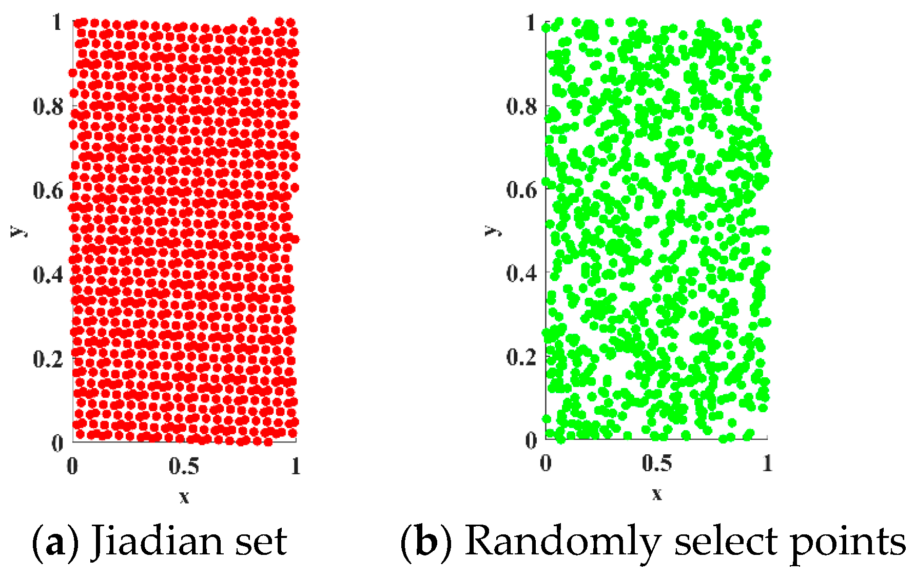
A.

Improvements in initialized populations.

COA by randomly generating the initial population is prone to uneven distribution of the population, which can lead to a reduction in the diversity of the population, poor quality of the population, and affect the convergence speed of the algorithm. Good point set is an effective method of uniform point selection. The theory was proposed by Mr. Hua Luogeng and has been applied in many swarm intelligent optimization algorithms. By the definition of the good point set, let $GD$ be a unit cube in a $D$-dimensional Euclidean space and, if $a\in GD$, the shape is:

$$p_n\left(k\right)=\{\left(\left\{a_1^{\left(n\right)}\times k\right\},\cdots ,\left\{a_i^{\left(n\right)}\times k\right\},1\le k\le n\right)$$

(10)

where $p_n\left(k\right)$ is the set of good points, $a$ is the good points, and $k$ is the number of samples.

Its deviation is satisfied as follows:

$$\varphi \left(n\right)=C\left(r,\epsilon \right)n^{-1+\epsilon }$$

(11)

where $C(a,\epsilon )$ is a constant, related only to $a,\epsilon$.

It has been shown theoretically that a weighted sum composed of $n$ good points has a smaller error than that obtained by employing any other $n$ points and is particularly suitable for approximate computations in high-dimensional spaces. As an example, in a two-dimensional unit search space, the comparison between random point taking and point taking by the good point set method is as follows.

Figure 1a shows the distribution of points in a two-dimensional unit search space ($0\le x\le 1$ and $0\le y\le 1$). The points are uniformly and densely distributed, indicating an optimal sampling method called the good point set, whereas Figure 1b points are randomly scattered and unevenly spaced, leading to a greater potential error in the computation. Therefore, the good point set method is particularly suitable for approximate computations in high dimensional spaces, as it can effectively cover the search space and reduce the potential errors in the computation.

B.

A dynamic reverse learning strategy is introduced to improve the quality of the initial population again:

$$X_d=X^{\ast }+r_1\times \left(r_2\times \left(U_b+L_b-X^{\ast }\right)-X^{\ast }\right)$$

(12)

where $X_{\mathrm{d}}$ is the individual after reverse learning, $X^{*}$ is the current individual, and $r_1$ and $r_2$ are random numbers from 0 to 1.

C.

The golden sine strategy is incorporated in the exploration phase of COA to enhance the global search capability of the algorithm; then, the mathematical model of tree-climbing long-nosed raccoon behavior is:

$$x_i^{t+1}\left(j\right)=x_i^t\left(j\right)\cdot \left|\sin R_1\right|+r_1\sin \left(2\pi r_2\right)\left(x_{\mathrm{best}}^t\left(j\right)-I\cdot x_i^t\left(j\right)\right)$$

(13)

As above, the ground long-nosed raccoon moves randomly according to the iguana’s landing position, which is mathematically modeled as:

$$I_{\mathrm{ground}}^t\left(j\right)=lb+r\cdot \left(ub-lb\right)$$

(14)

$$x_i^{t+1}\left(j\right)=\{\begin{array}{l}{x}_i^t\left(j\right)\cdot \left|\sin R_1\right|+r_1\sin \left(2\pi r_2\right)\left(I_{\mathrm{ground}}^t\left(j\right)-I\cdot x_i^t\left(j\right)\right)\\ \hspace{1em}\hspace{1em}\hspace{1em}\hspace{1em}\hspace{1em}\hspace{1em}\hspace{1em}\hspace{1em}\hspace{1em}\hspace{1em}\hspace{1em}\mathrm{if} f\left(I_{\mathrm{ground}}^t\right)<f\left(x_i^t\right)\\ x_i^t\left(j\right)\cdot \left|\sin R_1\right|+r_1\sin \left(2\pi r_2\right)\left(I\cdot x_i^t\left(j\right)-I_{\mathrm{ground}}^t\left(j\right)\right),\mathrm{else}\end{array}$$

(15)

$$i=\frac{N}{2}+1,\frac{N}{2}+2,\cdots ,N$$

(16)

where $I_{\mathrm{ground} }^t\left(j\right)$ is the iguana position, $r$ is a random number from 0 to 1, and $I$ is a random integer. $f(\ast )$ denotes the fitness value.

D.

In the development stage, four strategies, namely, soft encirclement of Harris Hawk, hard encirclement, soft encirclement of progressive fast dive, and hard encirclement of progressive fast dive, are fused, assuming that $S_p$ is the probability of escape of the prey, $S_p\in \left(\mathrm{0,1}\right)$, and that it can be escaped if $S_p<0.5$, and a random number E is also introduced:

• $S_p\ge 0.5$, $0.5\le E\le 1$; at this time, the soft envelope is implemented, and its position update formula is:

  $$U\left(t+1\right)=\Delta U\left(t\right)-E\left|J{U}_{\mathrm{prey}}\left(t\right)-U\left(t\right)\right|$$

  (17)

  $$\Delta U\left(t\right)=U_{\mathrm{prey}}\left(t\right)-U\left(t\right)$$

  (18)

  where $\mathsf{\Delta }U$ is the difference between the prey position and the individual position, $J~U$(0,2), $U\left(t\right)$ is the original position, and $U(t+1)$ is the updated position.
• $S_p\ge 0.5$ and $E<0.5$, at which point hard bracketing is implemented with the position update formula:

  $$U\left(t+1\right)=U_{\mathrm{prey}}\left(t\right)-E\left|\Delta U\left(t\right)\right|$$

  (19)
• $0.5\le E\le 1$ and $S_p<0.5$, at which time the soft envelopment of progressive fast swooping is implemented with the position update equation:

  $$\begin{array}{l}U\left(t+1\right)=Y=U_{\mathrm{prey}}\left(t\right)-E\left|J{U}_{\mathrm{prey}}\left(t\right)-U\left(t\right)\right|,f\left(Y\right)<f\left(U\left(t\right)\right)\\ U\left(t+1\right)=Z=Y+S\times L{e}^{\prime }vy\left(D\right),f\left(Z\right)<f\left(U\left(t\right)\right)\end{array}$$

  (20)
• $E<0.5$ and $S_p<0.5$; at this point in the hard envelope of real-time progressive fast swooping, the position update equation is:

  $$\begin{array}{l}U\left(t+1\right)=Y=U_{\mathrm{prey}}\left(t\right)-E\left|J{U}_{\mathrm{prey}}\left(t\right)-U_m\left(t\right)\right|,f\left(Y\right)<f\left(U\left(t\right)\right)\\ U\left(t+1\right)=Z=Y+S\times L{e}^{\prime }vy\left(D\right),f\left(Z\right)<f\left(U\left(t\right)\right)\end{array}$$

  (21)

E.

In the late iteration, in order to avoid the algorithm falling into the local optimum dilemma, this paper utilizes the vertical and horizontal crossover strategy to correct the individuals, the horizontal crossover to cross-search the population to reduce the search blind spots, and the vertical crossover to increase the diversity of the population while reducing the probability of the algorithm falling into the local optimum. However, although the vertical and horizontal crossover strategy has excellent search performance, the full-dimensional crossover operation will significantly increase the computational burden. In the face of high-dimensional problems, its computational cost will increase geometrically. Therefore, this paper adopts an unordered dimensional sampling method, which reduces the computational cost and also prevents the reduction in overall sparsity due to the reduction in the number of dimensions of the near-optimal individuals.

• The sampling rate determines the number of dimensions involved in the longitudinal crossover, and the dimensions involved are selected by the sampling rate, which is defined as follows:

$${\mathrm{Rate}}_{\mathrm{sample}}=\mathrm{ceil}\left(\max \left(\frac{t}{t_{\max }},{\epsilon }_1\right)\times D\right)$$

(22)

• Horizontal crossover is the process of selecting two individuals from the same dimension of the population and exchanging individual information at a certain randomized rate:

  $$M_{i,d}^{hc}=r_1\cdot F_{i,d}+\left(1-r_1\right)\cdot F_{j,d}+c_1\cdot \left(F_{i,d}-F_{j,d}\right)$$

  (23)

  $$M_{i,d}^{hc}=r_2\cdot F_{j,d}+\left(1-r_2\right)\cdot F_{i,d}+c_2\cdot \left(F_{j,d}-F_{i,d}\right)$$

  (24)
  where $M_{i,d}^{hc}$ and $M_{j,d}^{hc}$ are the $dth$ dimension of the offspring individuals $i$ and $j$ obtained after crossover, $F_{i,d}$ and $F_{j,d}$ are the dth dimensions of the parent individuals $F_i$ and $F_j$, and $c_1$ and $c_1$ are random numbers between –1 and 1, where the number of crossover dimensions is determined by the sampling rate.

• Longitudinal crossover refers to the exchange of dimensional information between different dimensions of the best individuals in the population according to a certain longitudinal crossover probability, thus generating a new generation of the best individuals to compete with their parents, which is conducive to the learning of different dimensions from each other and avoids the premature convergence of a certain dimension:

  $$M_{\mathrm{best},d_1}^{vc}=r\cdot F_{\mathrm{best},d_1}+\left(1-q\right)\cdot F_{\mathrm{best},d_2}$$

  (25)
  where $M_{\mathrm{best},d_1}^{vc}$ is the child obtained after crossover of the parent; again, the crossover dimension is determined by the sampling rate. $r$ is a random number from 0 to 1.

In order to reflect the practicality of the ICOA optimization algorithm designed in this paper, the test set function of the literature [24] is used for validation and the unoptimized COA is introduced to compare with the more mainstream DBO, GWO, WOA, and PSO optimization algorithms in recent years. The results are shown in Figure 2. From the Figure, it can be seen that the comprehensive performance of ICOA is better than other algorithms on all the test functions. This shows that ICOA is adaptable and superior in handling many optimization problems. Based on this, the parameters of ICOA in this paper are set as follows: the number of initialized populations is 20 and the maximum number of iterations is 10.

2.3. CNN Algorithm

Convolutional neural network (CNN) is a deep learning algorithm that is capable of taking an input image, assigning learnable weights and biases to different parts of the image, and being able to differentiate between them. The core foundation of the CNN is the convolutional layer, which, by applying a series of learnable filters to the input image, creates a feature map that summarizes the presence of the features detected in the input. Its mathematical expression is as follows [25].

Given an input image matrix $X$ and a filter matrix (also called a kernel), $F$, the convolution operation consists of sliding the filter across the input image. At each position, a matrix multiplication is performed, and the sum output of this multiplication forms a new matrix called the feature map $C$. This process can be represented as:

$$C\left(i,j\right)=\left(F\ast X\right)\left(i,j\right)={\displaystyle {\sum }_m{\displaystyle {\sum }_{n}F\left(m,n\right)\cdot X\left(i+m,j+m\right)}}$$

(26)

where $C\left(i,j\right)$ is the value of the feature map at position $\left(i,j\right)$; $\left(F\ast X\right)$ denotes the convolution of $F$ with $X$; and $F\left(m,n\right)$ represents the filter matrix with dimensions $m\times n$, which denotes the size of the filter. $X(i+m,j+n)$ represents the portion of the input image matrix currently covered by the filter.

Convolutional layers are usually followed by connecting pooling layers, which reduce computational complexity and overfitting by reducing the dimensionality of the feature map. After several convolutional kernel pooling layers, the probability distributions of different classes in the classification task are then obtained by passing through the fully connected layer kernel Softmax function. In this paper, the original Softmax layer is improved to SVM; Softmax, as a probabilistic method, is affected by outliers, whereas SVM uses the edges of the sample distribution to classify faulty samples within a certain distance and is more robust to outliers.

2.4. MSA Algorithm

MSA plays a central role in the Transformer model. It improves the model’s ability to process information about different locations by parallelizing the attention mechanism. The basic idea of MSA is to process the three matrices of query $\left(Q\right)$, key $\left(K\right)$, and value $\left(V\right)$ not only in a single attention space but separately in multiple parallel subspaces. Specifically, for each steal, there will be a different set of linear transformations of $Q$, $K$, and $V$. This can be realized by the weight matrices $W_h^Q$, $W_h^K$, and $W_h^V$, where $h$ denotes the index of the header. The output of the MSA is a splice of the results of these different processings, which are then subjected to a linear transformation. Mathematically, the MSA can be represented as [26]:

$$MultiHead\left(Q,K,V\right)=Concat\left(hea{d}_1,hea{d}_2,\cdots ,hea{d}_h\right)W^o$$

(27)

where the formula for each head, $hea{d}_h$, is:

$$hea{d}_h=Attention\left(Q{W}_h^Q,K{W}_h^K,V{W}_h^V\right)$$

(28)

And the computation of a single attention head can be expressed as:

$$Attention\left(Q,K,V\right)=soft\max \left(\frac{Q{K}^T}{\sqrt{d_K}}\right)V$$

(29)

where $d_K$ is the dimension of the key vector; this division operation is performed in order to scale the size of the dot product to prevent the gradient vanishing problem. $W_h^Q$, $W_h^K$, $W_h^V$, and $W^o$ are learnable parameter matrices used to transform the inputs to the appropriate space.

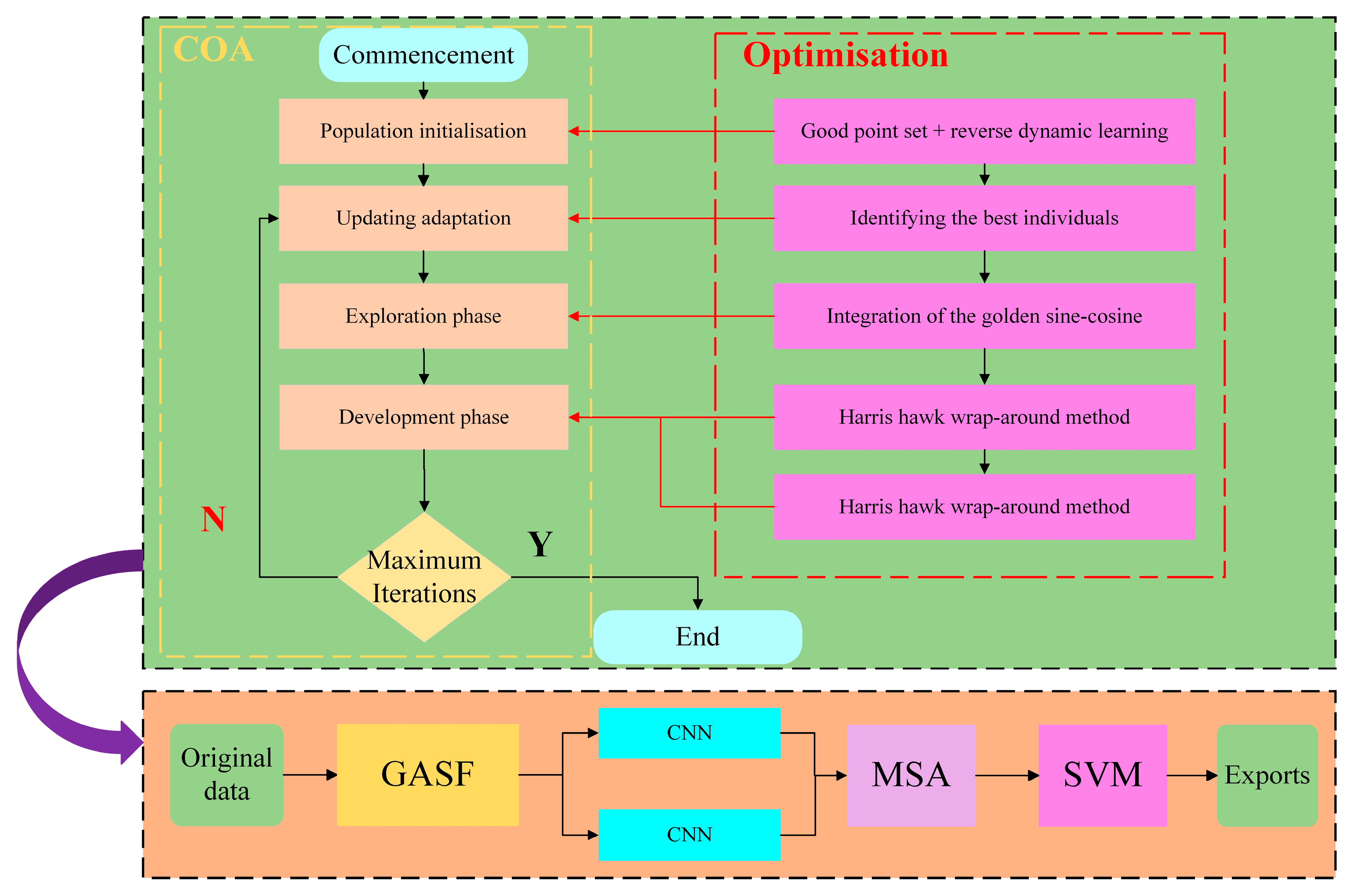
2.5. Rotor Fault Diagnosis Model Based on GASF and ICOA-PCNN-MSA-SVM

In this paper, GASF and ICOA-PCNN-MSA-SVM models are applied to the fault diagnosis of vibration signals of hydropower units. The original one-dimensional time series signal is converted into a two-dimensional image, and the image is input to the two-branch model at the same time, and the hyperparameters in the model are optimized by COA. In order to solve the problems of slow convergence and easily falling into the local optimal solution of COA, various strategies are used to optimize COA. Finally, the identification and classification of fault data are realized, and the flow chart of the model is shown in Figure 3.

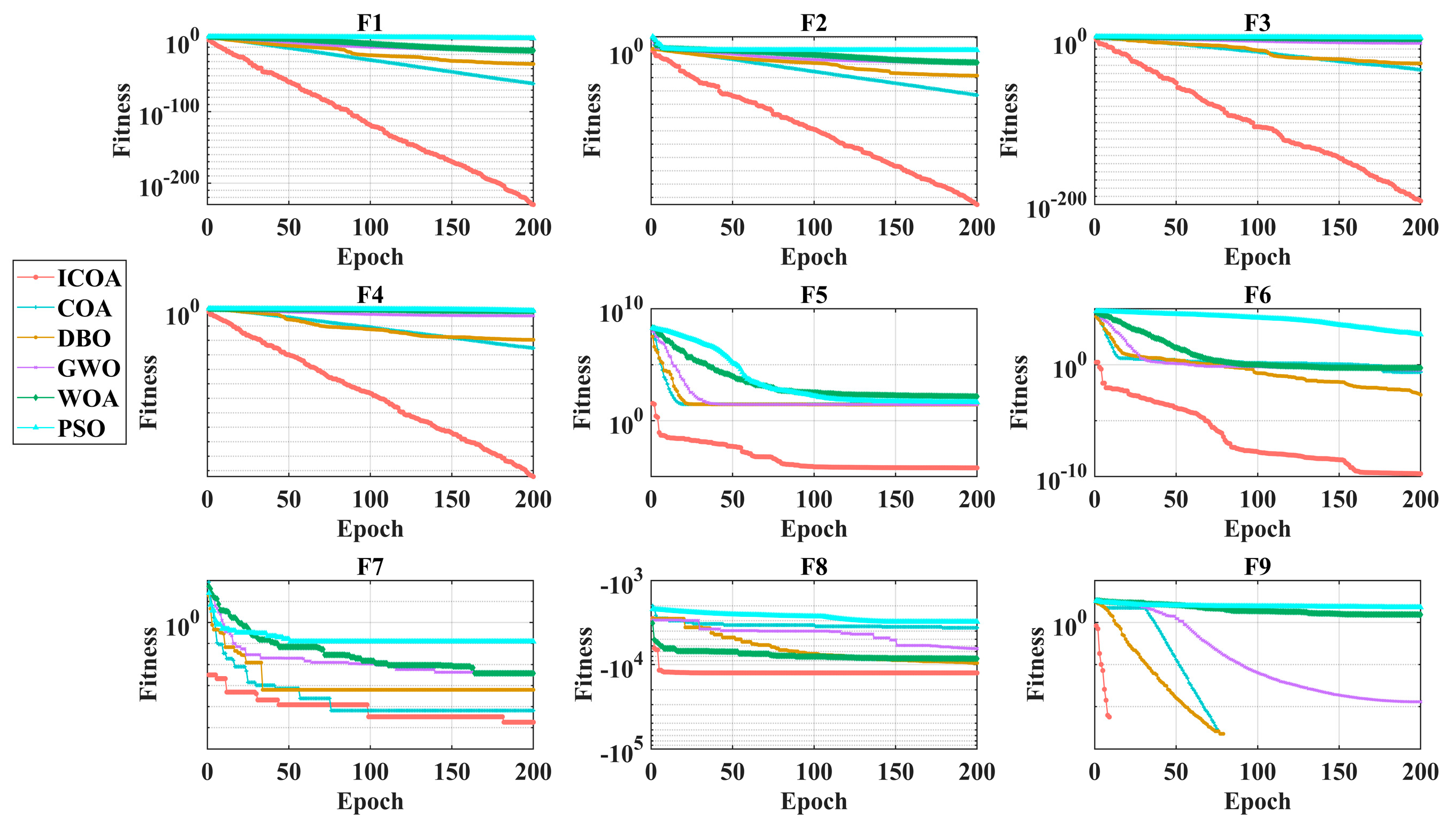
3. Simulation Verification 1

In this study, a hydraulic turbine failure analysis test platform was developed and constructed. As demonstrated in Figure 4, the platform consists of four key components: a water storage system, a water supply system, a test cell, and a water return system. The water storage system utilizes a tank to store water. The water supply system provides water through a pressure pump and several pipes. The test cell consists of a hydroelectric generator set.

On the other hand, the return system consists of a submersible pump and its pipes. The experiment aims to measure the acoustic vibration signals generated by the flow of sandy water through the turbine generator. The pre-experiment steps include filling the water tank and trough with water. When the experiment is started, the pressure pump and the submersible pump are activated simultaneously and the pressure pump pushes the water in the tank to flow through the pipes and impact the rotor blades inside the turbine. After the water flows through the turbine, it will flow back to the tank. Then, the submersible pump is responsible for pumping the water back into the water tank to ensure the continuity of the water cycle. Sediment is added to the tank to simulate conditions in the natural environment during the experiment. When the equipment was operated for a predetermined period, it was observed that the amplitude of the real-time signal collected by the sensors stabilized within a specific range and did not show any further increase. This phenomenon indicates that the sediment and water in the tank have reached an utterly homogeneous mixing state, allowing the collection and recording of signal data to begin.

The hydraulic turbine fault diagnosis experimental bench constructed in this paper is displayed in Figure 5, and the specific parameters of the hydraulic turbine generator set used are detailed in reference [27]. Meanwhile, this paper uses a noise sensor (model CRY2301) for signal acquisition, which is a miniaturized industrial-grade real-time spectrum analyzer equipped with an advanced digital signal processing (DSP) processor. It integrates a microphone, preamplifier, and data acquisition card to ensure accurate and efficient data processing while maintaining a compact design. Specific parameters regarding the noise sensor are detailed in

Table 1. Parameters of noise sensor CRY2301.

Parameter Name	Specifications	Unit
sampling rate	48	kHz
measurement frequency range	10–20,000	Hz
standard measurement range	25–130	dBA
measure dynamic range	≥110	dBA
communication interface	USB Audio + USB HID
size	25 × 115	mm

.

A total of 100 samples were measured in this experiment, which was divided into two kinds of working conditions, the healthy and sediment states, and the length of each sample was 2048. The specific waveforms are shown in Figure 6. The spectrum in Figure 6 shows that the eigenvalues of the two working conditions have apparent differences; the healthy state has low-frequency primary signals, while the sediment state has high-frequency primary signals. The original waveform is subjected to GASF transformation, and the result is shown in Figure 7.

The 2D feature map of the sediment condition presented in Figure 7b is obvious and the features are well recognizable compared to the healthy condition in Figure 7a. Among 100 sets of samples, they are divided into test sets and training sets according to the ratio of 2:8, 10 sets of samples for each condition in the test set and 40 sets of samples for each condition in the training set. The GSAF images are fed into each branch, and CNN performs feature extraction, and the extracted feature maps are demonstrated in Figure 8. The structure of the CNN network and the configuration of the parameters are described in detail in the reference [28].

The above figure shows the result of feature extraction using two-channel CNN. Only the four feature maps before and after each branch are shown for space reasons. Each subgraph presents a 2D heat map of different sample features, with the change in color representing the numerical strength of the features. Colors tending to red areas indicate higher feature intensity, while blue indicates lower feature intensity. The feature maps present the advantages of visualizing data features.

Accuracy is a measure of the number of samples predicted correctly by the model as a proportion of the total number of samples. It is a commonly used performance metric in classification tasks and is defined as follows:

$$\mathrm{Accuracy}=\frac{\mathrm{Number} \mathrm{of} \mathrm{correctly} \mathrm{predicted} \mathrm{samples}}{\mathrm{Total} \mathrm{number} \mathrm{of} \mathrm{samples}}$$

(30)

Loss value is a performance metric of a model during training or testing that measures the difference between the model prediction and the true value. Common loss functions are mean square error (MSE), cross entropy loss, etc. The smaller the loss value, the more accurate the model prediction. In this paper, MSE is used as the loss value, which is set as follows:

$$\mathrm{MSE}=\frac{1}{s}\sum _{i=1}^s{\left(y_i-{\widehat{y}}_i\right)}^2$$

(31)

where $y_i$ is the true value of the $ith$ sample, ${\widehat{y}}_i$ is the predicted value of the $ith$ sample, and $s$ is the total number of samples.

Figure 9 shows the iteration curves of the training set; with the increase in the number of iterations, the accuracy shows an overall increasing trend, indicating that the performance of the model is improving. The loss value, on the other hand, shows a de-creasing trend, which indicates that the model’s fit to the data is improving during the training process. Although the highest accuracy rate is about 90% after 240 iterations, the accuracy rate is further improved by the introduction of SVM, which can be the dataset to realize self-comparison and validation. In order to reflect the effectiveness and efficiency of the constructed model, two sets of models, ICOA-PCNN-SVM and ICOA-PCNN, are introduced for comparison. Their classification and identification are shown in Figure 10, where 1 and 2 in the vertical co-ordinates represent normal and sediment condition categories, respectively. Among them, the accuracy of the model designed in this paper reaches 100%, while the accuracy of ICOA-PCNN-SVM is 90% and that of ICOA-PCNN is 70%. Obviously, feature enhancement of MSA and self-validation of SVM play an important role in improving the accuracy.

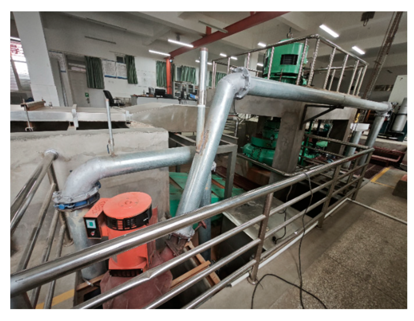
4. Simulation Verification 2

The literature [14] used a specially designed rotor failure test device to simulate and generate vibration data of a hydroelectric generating unit under four typical operating conditions: normal operation, wear and tear, rotor unbalance, and axial misalignment. To ensure the high quality and resolution of the data, the sampling rate of the vibration signals was set to 2048 Hz. A total of 360 samples of vibration signals under different conditions were recorded through this test facility. The waveforms are shown in Figure 11.

The original waveform is subjected to GASF transformation and the results are shown in Figure 12. Figure 12a shows the normal (NOR) waveform; Figure 12b shows the wear friction (FRI); Figure 12c shows the imbalance (IMB); and Figure 12d shows the misalignment (MSI). Comparing the four figures, it can be seen that the characteristic 2D images of different working conditions are all significantly different.

The 180 sets of samples are divided into test set and training set according to 2:8, where the test set samples are 9 sets for each working condition and the training set samples are 36 sets for each working condition. Separately, the GASF images are fed into each branch for CNN feature extraction, and the extracted feature maps are shown in Figure 13.

As seen from the above figure, there is a clear distinction between the colors of the CNN feature maps of different branches. Each feature map represents an activation feature at a different level of the input image renetwork, and the color of each map indicates a different activation intensity. Taking Figure 13a, for example, feature maps 1 and 2 have a similar visual style, consisting of large blocks of cool colors like blue and green, indicating that these converging features are less activated. Feature map 3 has more vibrant colors like pink and red, indicating that these regions are more significantly activated in the network. The colors here are more dispersed than the previous two feature maps, indicating more fine grain in the captured image features. Feature map 4 is quite different from the previous three maps in terms of color, dominated by yellow, orange, and green, with a much smoother color overlay and no distinct boundaries as in the previous ones. This indicates that the features captured by the CNN at this layer belong to different types. MSA further enhances the feature images, and the feature values of the two branches are merged and input into SVM for classification. The training curve is shown in Figure 14.

As seen from the above graph, the accuracy rate rises rapidly from a low point at the beginning, then reaches its first peak at about 10 iterations, gradually stabilizing and remaining at a high level. After about the first 10 iterations, there is a significant drop in accuracy, but it rebounds and stabilizes. The fluctuations in accuracy indicate that the model undergoes some adjustments during the early training phase. However, as learning progresses, the model stabilizes and reaches equilibrium at high accuracy. The loss value drops sharply in the early training period, showing that the model learns quickly in the first few iterations. Then, after about 10 iterations, the loss values level off and remain low, indicating that the model has a relatively small error after this point and that the training process is more stable. The remaining nine samples from the four operating conditions are put into the trained model as a test set for validation, and the results are shown in Figure 15.

In comparing model performance, the ICOA-PCNN-MSA-SVM model proposed in this paper performs consistently with the model in Simulation 1. The identification results of state classification are displayed in Figure 15. 1, 2, 3, and 4 are labeled in the horizontal co-ordinates of Figure 15, each representing one category of working conditions: NOR, FRI, IMB, and MSI. The accuracy rate of the ICOA-PCNN-MSA-SVM model under these four types of working conditions reaches the standard of 100%. In comparison, the accuracy of the compared models is 94.44% and 88.89% for these four conditions, respectively. This experimental result highlights the advantages of the two-branch design, which has a broader application potential and demonstrates higher performance. Especially when processing and analyzing complex data, this model design can capture the complexity and diversity of the data more effectively, thus enhancing the generalization of the model and data processing capability.

5. Conclusions

This paper proposes a hydroelectric unit fault diagnosis method based on the Gram summation field and ICOA-PCNN-MSA-SVM. Using the real machine test bed, the sound pattern data of runner wear and rotor fault platform data are obtained by dumping sediment for verification. The one-dimensional data are firstly converted into two-dimensional images using a Gram summation field. Then, the images are imported into a two-branch CNN network and, after merging, the feature images are classified using MSA and SVM. The experimental results show that the accuracy of the model faults designed in this paper is 100%. Through the above methods, the following conclusions are obtained:

(1)

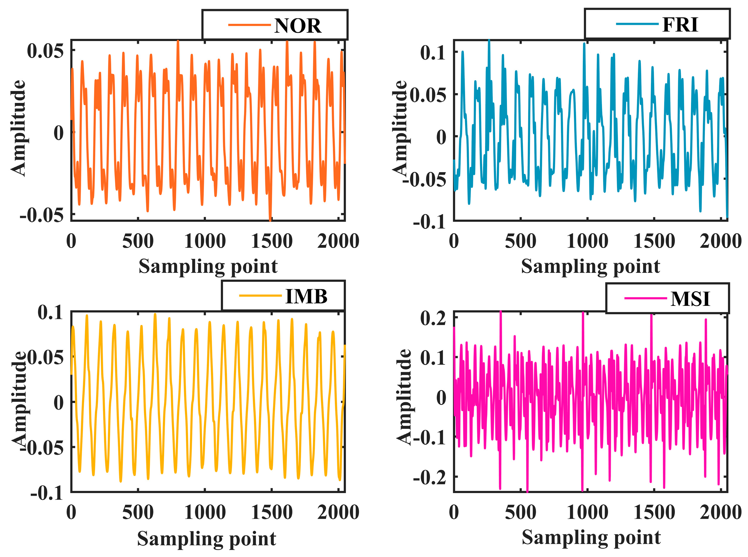
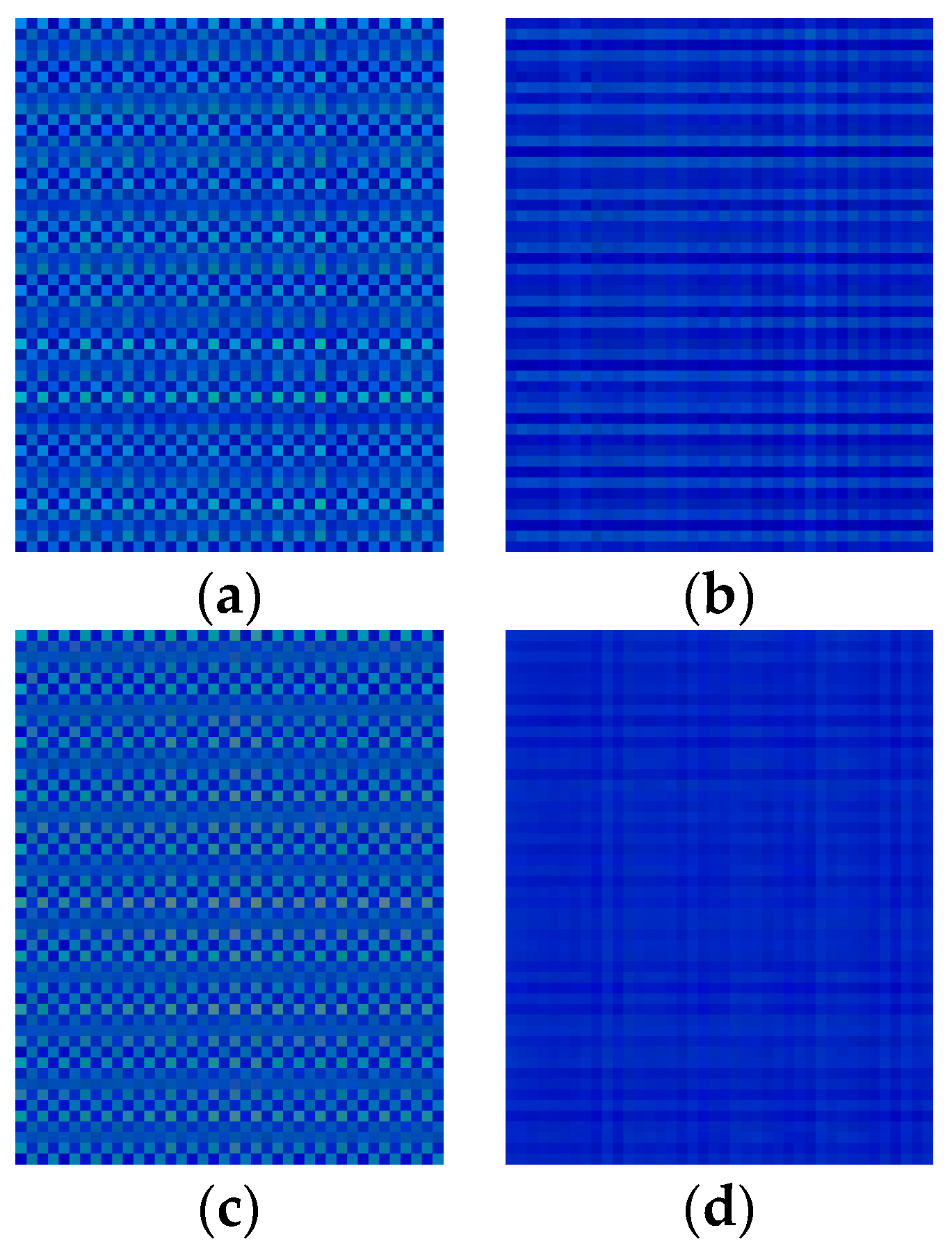
Converting one-dimensional time series signals into two-dimensional images helps extract richer and more distinguishable features.

(2)

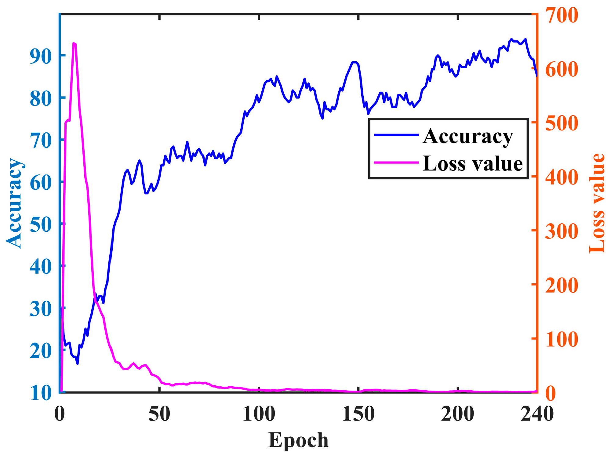
ICOA can optimize the learning rate, convolution kernel size, and other parameters in the model, which makes the model more reasonable and effectively improves the fault recognition accuracy.

(3)

A double-branching design can make the CNN learn different weight values. The two branching high-dimensional features complement each other, which significantly enhances the deep spatial features. Replacing the SVM with the Softmax layer in the CNN and introducing the MSA to focus on feature reinforcement makes the model more robust to outliers and improves the accuracy of fault recognition.

The method proposed in this paper performs well regarding diagnostic efficiency and robustness. It can serve as a valuable supplement to the hydropower unit’s fault detection techniques. This study provides critical technical support for the fault diagnosis of hydropower units and demonstrates its high value in engineering applications.

References

1. Villeneuve, Y.; Séguin, S.; Chehri, A. AI-Based Scheduling Models, Optimization, and Prediction for Hydropower Generation: Opportunities, Issues, and Future Directions. Energies 2023, 16, 3335. [Google Scholar] [CrossRef]
2. Piwowar, A.; Dzikuć, M. Water energy in Poland in the context of sustainable development. Energies 2022, 15, 7840. [Google Scholar] [CrossRef]
3. Morcillo, J.D.; Angulo, F.; Franco, C.J. Analyzing the hydroelectricity variability on power markets from a system dynamics and dynamic systems perspective: Seasonality and ENSO phenomenon. Energies 2020, 13, 2381. [Google Scholar] [CrossRef]
4. Kulpa, J.; Kopacz, M.; Stecuła, K.; Olczak, P. Pumped Storage Hydropower as a Part of Energy Storage Systems in Poland—Młoty Case Study. Energies 2024, 17, 1830. [Google Scholar] [CrossRef]
5. Palma, L. Hybrid Approach for Detection and Diagnosis of Short-Circuit Faults in Power Transmission Lines. Energies 2024, 17, 2169. [Google Scholar] [CrossRef]
6. Li, X.; Zeng, Y.; Qian, J.; Xiao, B.; Fei, N.; Dao, F.; Zou, Y. Modeling new nature of extraction and state identification of vibration shock signals from hydroelectric generating units using LCGSA optimized RBF combined with CEEMDAN sample entropy. IEEE Access 2024. [Google Scholar] [CrossRef]
7. Wang, Y.; Zou, Y.; Hu, W.; Chen, J.; Xiao, Z. Intelligent fault diagnosis of hydroelectric units based on radar maps and improved GoogleNet by depthwise separate convolution. Meas. Sci. Technol. 2023, 35, 025103. [Google Scholar] [CrossRef]
8. Dao, F.; Zeng, Y.; Zou, Y.; Li, X.; Qian, J. Acoustic vibration approach for detecting faults in hydroelectric units: A review. Energies 2021, 14, 7840. [Google Scholar] [CrossRef]
9. Xu, B.; Li, H.; Pang, W.; Chen, D.; Tian, Y.; Lei, X.; Gao, X.; Wu, C.; Patelli, E. Bayesian network approach to fault diagnosis of a hydroelectric generation system. Energy Sci. Eng. 2019, 7, 1669–1677. [Google Scholar] [CrossRef]
10. Zheng, Y.; Pan, T.; Wang, H.; Ge, X.; Zhang, Y. Application Study of Improved EMD-ICA Denoising in Hidden Rubbing Diagnosis of Hydraulic Turbine Units. J. Vib. Shock 2017, 36, 235–240. [Google Scholar]
11. Hu, X.; Xiao, Z.; Liu, D.; Jiang, W.; Liu, D. Fault Diagnosis of Hydroelectric Units Based on VMD-CNN. Hydropower Energy Sci. 2020, 38, 137–141. [Google Scholar]
12. Fu, Z.; Yin, G.; Zhu, J.; Yuan, Y. Study on Degradation Prediction Method for Hydroelectric Units Based on EEMD and LSTM. J. Sol. Energy 2022, 43, 75–81. [Google Scholar]
13. Chen, F.; Wang, B.; Zhou, D.; Zhao, Z.; Ding, C. Fault Diagnosis Method for Hydroelectric Unit Shaft System Integrating Improved Symbolic Dynamic Entropy and Random Configuration Network. J. Hydraul. Eng. 2022, 53, 1127–1139. [Google Scholar]
14. Chen, F.; Wang, B.; Liu, T.; Zhang, W.; Gao, Y. Fault Diagnosis of Hydroelectric Units Based on Time-Shifted Multi-scale Attention Entropy and Random Forest. J. Hydraul. Eng. 2022, 53, 358–368+378. [Google Scholar]
15. Hu, M.; Yang, X.; Huang, J.; Hu, J.; Wang, C. Fault Diagnosis Method Based on MTF-ResDSCNN Two-Dimensional Images. Mech. Transm. 2024, 48, 170–176. [Google Scholar]
16. Li, G.; Ao, J.; Hu, J.; Liu, Y.; Huang, Z. Dual-source gramian angular field method and its application on fault diagnosis of drilling pump fluid end. Expert Syst. Appl. 2024, 237, 121521. [Google Scholar] [CrossRef]
17. Cui, J.; Zhong, Q.; Zheng, S.; Peng, L.; Wen, J. A lightweight model for bearing fault diagnosis based on gramian angular field and coordinate attention. Machines 2022, 10, 282. [Google Scholar] [CrossRef]
18. Ding, C.; Wang, Z.; Ding, Q.; Yuan, Z. Convolutional neural network based on fast Fourier transform and gramian angle field for fault identification of HVDC transmission line. Sustain. Energy Grids Netw. 2022, 32, 100888. [Google Scholar] [CrossRef]
19. Amiri, A.F.; Kichou, S.; Oudira, H.; Silvestre, S. Fault detection and diagnosis of a photovoltaic system based on deep learning using the combination of a convolutional neural network (cnn) and bidirectional gated recurrent unit (Bi-GRU). Sustainability 2024, 16, 1012. [Google Scholar] [CrossRef]
20. Hadroug, N.; Iratni, A.; Hafaifa, A.; Alili, B. Implementation of vibrations faults monitoring and detection on gas turbine system based on the support vector machine approach. J. Vib. Eng. Technol. 2024, 12, 2877–2902. [Google Scholar] [CrossRef]
21. Li, Y.; Liu, W.; Huang, D. Image Denoising Network Model Integrating Multi-Head Attention Mechanism. Comput. Sci. 2023, 50, 326–333. [Google Scholar]
22. Memarian, A.; Damarla, S.K.; Memarian, A.; Huang, B. Detection of poor controller tuning with Gramian Angular Field (GAF) and StackAutoencoder (SAE). Comput. Chem. Eng. 2024, 185, 108652. [Google Scholar] [CrossRef]
23. Dehghani, M.; Montazeri, Z.; Trojovská, E.; Trojovsky, P. Coati Optimization Algorithm: A new bio-inspired metaheuristic algorithm for solving optimization problems. Knowl. -Based Syst. 2022, 259, 110011. [Google Scholar] [CrossRef]
24. Zhu, X.; Wang, T.; Lai, Z. Gold Jackal Optimization Algorithm Improved by Hybrid Strategy. Comput. Eng. Appl. 2024, 60, 99–112. [Google Scholar]
25. Goumiri, S.; Benboudjema, D.; Pieczynski, W. A new hybrid model of convolutional neural networks and hidden Markov chains for image classification. Neural Comput. Appl. 2023, 35, 17987–18002. [Google Scholar] [CrossRef] [PubMed]
26. Ghazimoghadam, S.; Hosseinzadeh, S.A.A. A novel unsupervised deep learning approach for vibration-based damage diagnosis using a multi-head self-attention LSTM autoencoder. Measurement 2024, 229, 114410. [Google Scholar] [CrossRef]
27. Dao, F.; Zeng, Y.; Qian, J. Fault diagnosis of hydro-turbine via the incorporation of bayesian algorithm optimized CNN-LSTM neural network. Energy 2024, 290, 130326. [Google Scholar] [CrossRef]
28. Xiao, B.; Zeng, Y.; Dao, F.; Zou, Y.; Li, X. EEMD-CNN Integrated Hydropower Unit Rubbing Fault Acoustic Fingerprint Recognition Model. J. Hydroelectr. Eng. 2024, 43, 59–69. [Google Scholar]
Figure 1. Comparison of random sampling and optimal sampling method.
Energies 17 03084 g001
Figure 2. Comparative test function set.
Energies 17 03084 g002
Figure 3. Flowchart.
Energies 17 03084 g003
Figure 4. Operational process of the hydro turbine fault test bench.
Energies 17 03084 g004
Figure 5. Hydro turbine fault diagnosis test bench.
Energies 17 03084 g005
Figure 6. Acoustic vibration actual measurement signal and spectrum.
Energies 17 03084 g006
Figure 7. GASF images of acoustic vibration actual measurement signals in healthy and sediment conditions. (a) GASF images in a health condition. (b) GASF images in a sediment condition.
Energies 17 03084 g007
Figure 8. First and last four CNN feature maps of acoustic vibration branches 1 and 2. (a) The first four feature maps of the first branch road. (b) Four feature maps after the first branch road. (c) The first four feature maps of the second branch road. (d) Four feature maps after the second branch road.
Energies 17 03084 g008aEnergies 17 03084 g008b
Figure 9. Training set iteration curve.
Energies 17 03084 g009
Figure 10. Fault classification results of acoustic vibration signals.
Energies 17 03084 g010
Figure 11. Rotor fault waveform diagram.
Energies 17 03084 g011
Figure 12. GASF images of original waveform in healthy, wear, imbalance, and misalignment conditions. (a) GASF image of NOR. (b) GASF image of FRI. (c) GSAF image of IMB. (d) GASF image of MSI.
Energies 17 03084 g012
Figure 13. First and last four CNN feature maps of rotor vibration fault branches 1 and 2. (a) The first four feature maps of the first branch road xxx. (b) Four feature maps after the first branch road. (c) The first four feature maps of the second branch road. (d) Four feature maps after the second branch road.
Energies 17 03084 g013
Figure 14. Training iteration curve.
Energies 17 03084 g014
Figure 15. Rotor vibration fault classification.
Energies 17 03084 g015