Multi-Objective Optimization towards Heat Dissipation Performance of the New Tesla Valve Channels with Partitions in a Liquid-Cooled Plate

Abstract

The utilization of liquid-cooled plates has been increasingly prevalent within the thermal management of batteries for new energy vehicles. Using Tesla valves as internal flow channels of liquid-cooled plates can improve heat dissipation characteristics. However, conventional Tesla valve flow channels frequently experience challenges such as inconsistencies in heat dissipations and unacceptably high levels of pressure loss. In light of this, this paper proposes a new type of Tesla valve with partitions, which is used as internal channel for liquid-cooled plate. Its purpose is to solve the shortcomings of existing flow channels. Under the working conditions of Reynolds number equal to 1000, the neural network prediction-NSGA-II multi-objective optimization method is used to optimize the channel structural parameters. The objective is to identify the optimal structural configuration that exhibits the greatest Nusselt number while simultaneously exhibiting the lowest Fanning friction factor. The variables to consider are the half of partition thickness H, partition length L, and the fillet radius R. The study result revealed that the optimal parameter combination consisted of H = 0.25 mm, R = 1.253 mm, L = 0.768 mm, which demonstrated the best performance. The Fanning friction factor of the optimized flow channel is substantially reduced compared to the reference channel, reducing by approximately 16.4%. However, the Nusselt number is not noticeably increased, increasing by only 0.9%. This indicates that the optimized structure can notably reduce the fluid’s friction resistance and pressure loss and slightly enhance the heat dissipation characteristics.

1. Introduction

In recent decades, the growing consumption of non-renewable energy sources and the intensification of the use of fossil fuels have become widely recognized as pressing and consequential global concerns [1]. One of the primary consumers of fossil fuels is the transport sector [2]. The industry is gradually phasing out conventional internal combustion engines and replacing them with electric vehicles (EVs) and hybrid vehicles (HEVs). Lithium batteries (Li-ion) are a key component in new energy vehicles, and researchers have been drawn to this field. Li-ion batteries possess several advantages, including high specific energy, long life, and stable voltage [3]. However, their performance is highly dependent on the working temperature, with significant deterioration observed under temperatures below or above the optimal range [4]. It is crucial, therefore, to ensure optimal performance from Li-ion batteries by maintaining adequate temperature regulation through the integrated battery thermal management system (BTMS).

BTMS can be categorized into three types according to the cooling medium being utilized: air cooling, phase change material (PCM) cooling, and liquid cooling [5]. Air cooling is the most cost-effective and reliable option, but its heat dissipation efficiency is inferior to other cooling methods. PCM is still in its infancy and requires further research in the field of materials to enhance its reliability. Liquid cooling is currently the dominant area of research due to its efficient cooling performance [6,7,8].

The primary cooling method for the battery system is the circulation of a coolant within the liquid-cooled plate. This coolant is responsible for cooling the battery [9]. The shape and design of the liquid-cooled plate’s channel is critical to achieving optimal cooling performance [10]. The most commonly utilized liquid-cooled plate channel structure encompasses a variety of configurations, including serpentine channels [11,12], micro-channels [13], leaf-shaped channels [14], and so forth. Given the great potential for further increasing the thermal performance of these channel structures, there has been an ongoing focus on the refinement and improvement of the optimal design of these structures.

A range of factors contribute to the thermal performance of liquid-cooled panels. The multi-objective optimization method can be employed to significantly enhance the thermal performance of liquid-cooled plate. Widely used multi-objective optimization algorithms include genetic algorithm [15], topology optimization algorithm [16], the orthogonal test method [17], etc. These multi-objective optimization algorithms have achieved good results for different channel structures. Fan et al. [18] proposed a double-layer dendritic channel for liquid-cooled panels with multi-objective optimization using a genetic algorithm, which resulted in a significant improvement over the traditional serpentine channel. Yuan et al. [19] employed topology optimization, which significantly enhanced the performance of the liquid-cooled plate channel structure and reduced pressure drop. However, the improvement in cooling performance was not statistically significant. Additionally, there was a significant correlation between the cooling performance and the conditions of use. In order to identify the optimal combination of parameters for liquid-cooled plate channels, Shang et al. [20] employed orthogonal experiments. This approach enabled them to achieve lower temperature bounds and cell temperature uniformity, while also reducing pump consumption.

Integrating a surrogate model with the optimization algorithm for optimization is an efficient design strategy [21]. The surrogate model refers to the computational model that predicts unknown experimental results based on existing datasets. Commonly used surrogate models include response surface, linear regression, radial basis function (RBF), Kriging, support vector regression (SVR), and artificial neural network (ANN) [22]. Multilayer perceptron (MLP) is a feedforward ANN [23] and has been shown to have strong predictive ability in some studies. Kim et al. [24], based on high-spatial-resolution optical fiber temperature measurement data [24] from quenching, utilized three models—SVR, MLP, and random forest (RF). The results displayed a significant improvement of the model performance through the application of MLP. This model had the best prediction accuracy, further strengthening the assumption of its effectiveness in predicting quenching phenomena. Mudawar et al. [25] applied the MLP model to flow boiling data collected in microgravity and Earth gravity. The model demonstrated superior prediction accuracy in each subset of the database. The quality of the optimization results highly depends on the selected multi-objective optimization algorithm. Two commonly used algorithms are the non-dominated sorting genetic algorithm II (NSGA-II) and the strength Pareto evolutionary Algorithm 2 (SPEA2) [26]. As early as 2009, the research of Gosselin et al. [27] reviewed the application of the NSGA-II in the field of heat transfer, and since then, the NSGA-II has been widely utilized in optimization problems in the field of heat transfer. Pan et al. [28] employed NSGA-II for the multi-objective optimization of bionic fractal heat transfer structures. The study revealed that the optimized structures exhibited lower power consumption and superior heat transfer performance. Sun et al. [29] used NSGA-II to optimize the multi-objective parameters of the trapezoidal outrigger segmented thermoelectric generator, which provided guidance for the subsequent design. Yildizeli et al. [30] used NSGA-II to optimize the parameters of the microchannel radiator, and the results showed that in most optimal cases, the height of the microchannel is recommended to be in the range of 0.50 to 0.67 mm. The above work proves the superiority of MLP and NSGA-II, and the optimization method combined with these two methods can provide guidance for structural design.

The Tesla valve, a check valve initially designed by N. Tesla in 1920 [31], is an excellent choice for incorporation into microchannel structures as it features no moving parts, reducing the risk of mechanical failure and enabling efficient and reliable operation [32,33]. Vries et al. [34] combined the new Tesla valve with a heat pipe to increase the thermal resistance of a conventional heat pipe and was demonstrated to achieve a 14% reduction in thermal resistance when compared to a traditional heat pipe. The novel multi-stage Tesla Valve liquid-cooled plate structure proposed by Monika et al. [35] that significantly improves the heat transfer performance of the liquid-cooled plate results in an increase in pressure drop. Considering the intricate design of the Tesla valve, it is natural that the pressure drop at the fluid interface would increase, but it remains possible to optimize its structural parameters to achieve an optimal balance between heat transfer performance and pressure drop.

However, the application of Tesla valves to liquid-cooled plate channel structures has been less well studied, and most optimization work has been carried out using empirical or semi-empirical designs to obtain optimization patterns. The advantage of this approach is that it requires less computational effort and fewer samples, but it can lead to the problem of non-uniform samples and incomplete reflection of features. To address this, this paper proposes a partition Tesla valve structure that can be employed for the internal channel of the liquid-cooled plate. A parameter optimization model is constructed using MLP prediction combined with NSGA-II. The input to this model contains half of partition thickness H, partition length L, and fillet radius R. The output contains information about two crucial characteristics of the selected structure: its Nusselt number in comparison with the reference structure and the Fanning friction factor in relation to the reference structure. Our goal is to identify the best possible mix of the three design elements H, Land, and R that yield a superior structural design that efficiently delivers a high Nusselt number and a low Fanning friction factor compared to the existing benchmark design. The optimization results are then examined for their accuracy, and an analysis is conducted on how sensitive the input parameters are to the output parameters. A comparison is then made between the heat dissipation performance and flow characteristics of the optimal structure and the reference structure.

2. Physical Model and Numerical Methods

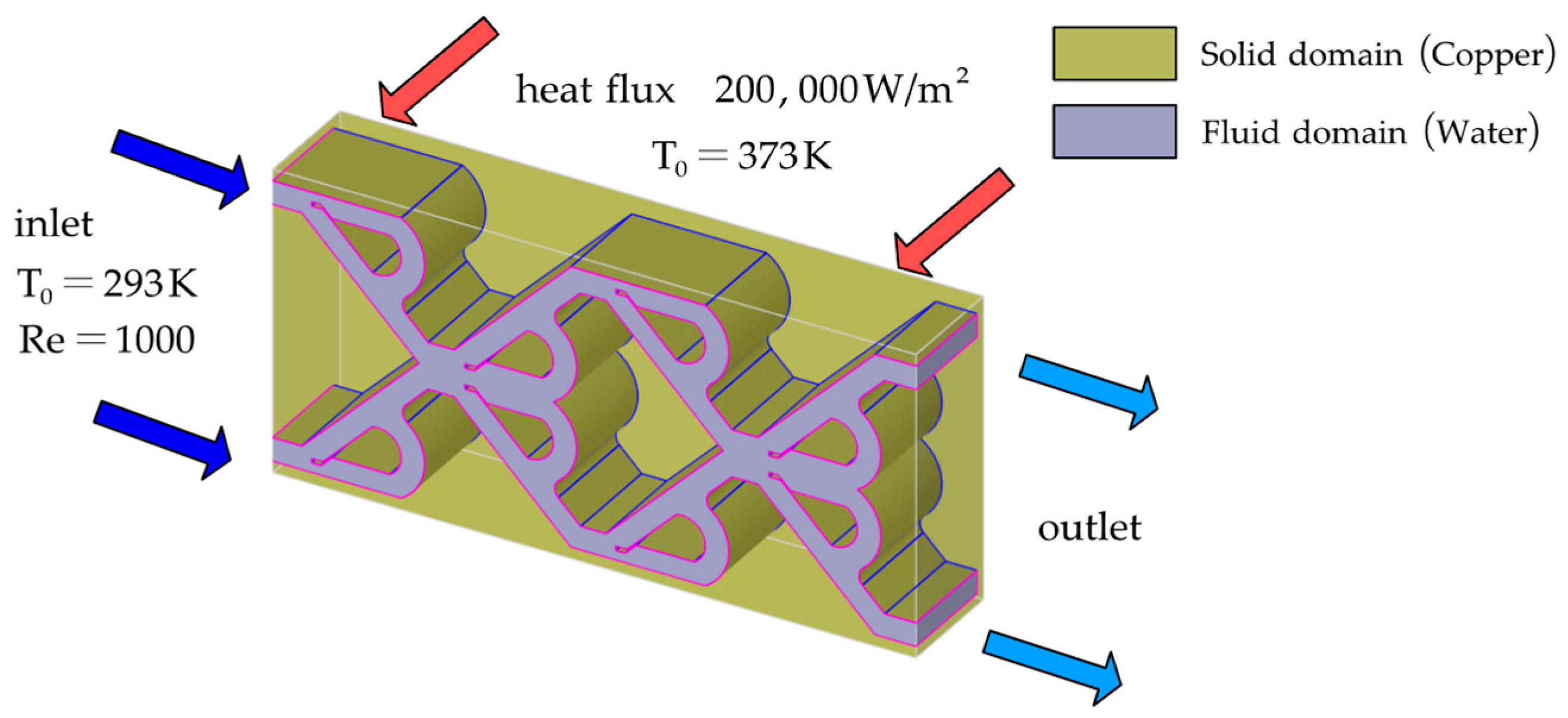
2.1. Physical Model

The primary objective of this research project is to construct an innovative liquid-cooled plate that incorporates a Tesla valve as a crucial internal component. The main purpose of this study is to construct a substitute model that accurately represents the values of the design variables and the fluid dynamic parameters Nu and f, using the acquired numerical simulation data. Subsequently, a multi-objective optimization approach will be utilized using this surrogate model. The goal is to identify a design feature that exhibits a high Nu value and a low f value simultaneously. This study employs a physical model, shown in Figure 1, with four views: (a) an isometric view, (b) a main view, and (c) a schematic view of its internal channels, (d) reference structure. In Figure 1a, the overall dimensions of the liquid-cooled plate are labeled. Figure 1b provides additional details on the specific dimensions of the channel. Notably, the fillets are integral design elements in this study. Due to the use of an array and symmetry, there are eight fillets as design points in the physical model, which are kept equal. Figure 1c then labels the fine dimensions of the internal channels; Figure 1d represents the reference structure for this study. Du et al. [36] have confirmed the effectiveness of a similar design in this study, specifically for liquid-cooled panels, with the exception of the channel without partitions. The purpose of the optimization process is to identify the most effective values for the parameters and structure. The remaining parameters and the structure to be optimized will remain unchanged. The innovative feature is the introduction of a rectangular partition at the front of the Tesla valve. This partition serves as a design parameter, and its length (L) and height (H) define the physical dimensions of the partition. The physical model features eight identical partitions, each with its equally own length and height.

2.2. Numerical Methods and Data Reduction

The incompressible Reynolds time-averaged Navier–Stokes equations in 3D were solved using the FLUENT module of ANSYS 18.0 software. Details on the continuity, momentum, and energy equations can be found in Ref. [37]. It can be seen from Ref. [35] that laminar flow is present in Tesla valve microchannel structures only at Re ≤ 300. In this study, the Re value is equal to 1000, so the turbulence model was used for the calculations. Ref. [38] demonstrates that the renormalization group turbulence model $RNG k-\epsilon$ performs well in simulating the fluid flow and heat transfer characteristics in turbulent channels. Therefore, the $RNG k-\epsilon$ turbulence model is chosen for numerical simulation in this calculation. The solver was chosen to be the semi-implicit SIMPLEC algorithm in FLUENT for the pressure-dependent equations, the momentum equation was established, and the discrete format of the energy equation was adjusted to the second-order windward format. The results are considered converged when the residuals of energy, velocity, continuity, k parameter, and $\epsilon$ parameter converge to ${10}^{-6}$. Continuity, momentum, and energy of fluid flow are all expressed as follows:

$$\frac{\partial }{\partial x_i}(\rho u_i)=0$$

(1)

$$\frac{\partial }{\partial x_i}(\rho u_i{u}_k)=\frac{\partial }{\partial x_i}(\eta \frac{\partial u_k}{\partial x_i})-\frac{\partial p}{\partial x_k}$$

(2)

$$\frac{\partial }{\partial x_i}(\rho u_{i}T)=\frac{\partial }{\partial x_i}(\frac{\lambda }{c_p}\frac{\partial T}{\partial x_i})$$

(3)

where $\rho$ is the density of fluid; $u_i$ is the velocity of vector; $\eta$ is the viscosity; $p$ is the pressure; $T$ is the temperature; $\lambda$ is the thermal conductivity of the fluid; $c_p$ is the specific heat capacity at constant pressure; $k$ is the turbulent kinetic energy equation; and $\partial$ is the diffusion equation. Additionally, the diffusion equation is used to represent the phenomenon of heat transfer. The equation of energy conservation of solid is as follows:

$$k_s{\nabla }^2{T}_s=0$$

(4)

where $k_s$ represents the thermal conductivity of the solid and $T_s$ represents the temperature of the solid.

Lastly, the turbulence model used in this simulation is as follows:

$$\frac{\partial }{\partial t}(\rho k)+\frac{\partial }{\partial x_i}\left(\rho k{u}_i\right)=\frac{\partial }{\partial x_j}\left({\alpha }_k{\mu }_{eff}\frac{\partial k}{\partial x_j}\right)+G_k+G_b-\rho \epsilon -Y_M$$

(5)

$$\frac{\partial }{\partial t}(\rho \epsilon )+\frac{\partial }{\partial x_i}\left(\rho \epsilon u_i\right)=\frac{\partial }{\partial x_j}\left({\alpha }_{\epsilon }{\mu }_{eff}\frac{\partial \epsilon }{\partial x_j}\right)+C_{1\epsilon }\frac{\epsilon }{k}\left(G_k+C_{3\epsilon }{G}_b\right)-C_{2\epsilon }\rho \frac{{\epsilon }^2}{k}-R_{\epsilon }$$

(6)

where $G_k$ denotes the turbulent kinetic energy attributed to the laminar velocity gradient, $G_b$ is the source of the turbulent kinetic energy is the buoyancy effect, $Y_m$ is the transition in compressible turbulence experiences fluctuations attributed to diffusion, and ${\alpha }_k$ and ${\alpha }_{\epsilon }$ are turbulence reaction Prandtl numbers for the k and $\epsilon$ equations, respectively.

The Reynolds number can be calculated by applying the following equation:

$$\mathrm{Re}=\frac{{\rho }_1{v}_1{D}_H}{{\mu }_1}$$

(7)

where ${\rho }_1$ is the density of fluid; $v_1$ is the fluid flow rate of inlet; ${\mu }_1$ is the fluid viscosity; and $D_H$ is the hydraulic diameter, which can be obtained through the equation below as well:

$$D_H=\frac{4A_{in}}{C_{in}}$$

(8)

where $A_{in}$ is the area of the entrance to the rectangular section and $C_{in}$ is the perimeter of the entrance to the rectangular section.

The effective heat flux can be calculated by the following formula:

$$q_{eff}=\frac{q_{heat}{A}_{heat}}{A_{\mathrm{int}}}$$

(9)

where q_heat is the constant heat flux from the heat source, A_heat is the area of the heat source surface, and A_int is the surface area of the boundary between a solid and a liquid.

The average heat transfer coefficient is estimated using the following formula:

$$h_{ave}=\frac{q_{eff}}{T_{ave}-(T_{\mathrm{int}}-T_{out})/2}$$

(10)

where T_ave is the area-weighted average temperature of the heat source surface, T_int is the inlet area-weighted average temperature, and T_out is the outlet area-weighted average temperature.

The Nusselt number is calculated via the following equation:

$$Nu=\frac{h_{avre}{D}_H}{k_1}$$

(11)

where k₁ is the thermal conductivity of the fluid.

The pressure drop is calculated by the following equation:

$$p_{drop}=p_{\mathrm{int}}-p_{out}$$

(12)

where p_int is the area-averaged pressure at the inlet and p_out is the area-averaged pressure at the outlet.

The Fanning friction factor is calculated by the following equation:

$$f=\frac{p_{drop}{D}_H}{2{\rho }_{1}L{v}_1^2}$$

(13)

where L is the feature length.

2.3. Boundary Conditions and Assumptions

The locations of the inlet, outlet, and heat source are depicted in Figure 2. The inlet, located at the bottom of the model, is designed as a velocity inlet, while the outlet, situated at the top, is designated as a pressure outlet. In this study, Re was set to 1000 to analyze channel structure performance. The Reynolds number was used to determine the entrance flow velocity, which was found to be 0.31 m/s. The inlet temperature was set at 293 K, while the initial state of the heat source was fixed at 373 K, with a heat flux of 200,000 W/m² [39]. Figure 2 illustrates the computational domain of the employed physical model for this research. The solid domain material was set to copper, the fluid was set to water, and the material property parameters are listed in

Table 1. Material properties.

Material	$\mathit{\rho } (\mathbf{k}\mathbf{g}/{\mathbf{m}}^3)$	Cp (J/kg·K)	$\mathit{\lambda } (\mathbf{W}/\mathbf{m}·\mathbf{K})$	$\mathit{\mu } (\mathbf{k}\mathbf{g}/\mathbf{m}·\mathbf{s})$
Copper	8978	381	387.6
Water	998.2	4182	0.6	0.001003

.

In order to streamline the computational model and guarantee the precision of the outcomes, the following suppositions were upheld throughout this study:

(a)

Gravity is negligible;

(b)

The working fluids and solids are incompressible;

(c)

Radiant heat transfer is negligible;

(d)

The material is thermophysically stable;

(e)

Heat source surface thickness of 1 mm.

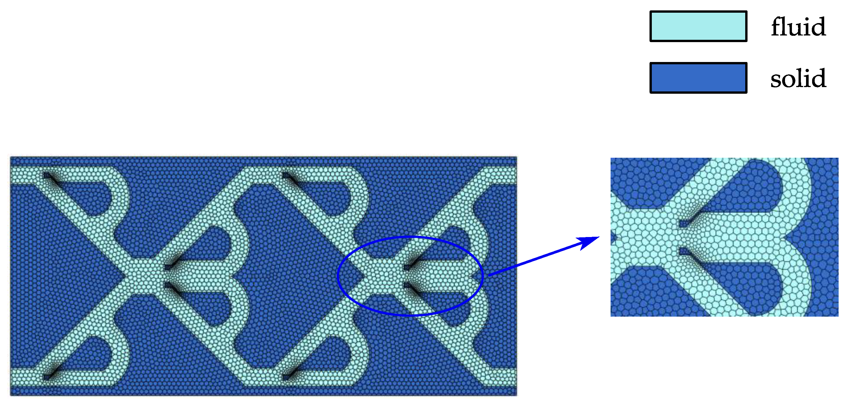
2.4. Grid Independence and Validation of Results

In numerical simulations, the accuracy of the computational results is significantly influenced by the number and quality of meshes. Figure 3 depicts a schematic diagram of the grid division. In this study, the FLUENT MESHING module was employed for the generation of the mesh. This study uses unstructured meshes for meshing, keeping the minimum surface mesh size unchanged at 0.1 mm, and increasing the number of meshes by controlling the maximum surface mesh size to gradually shrink from 0.5 mm. Set 10 layers of boundary layer to capture boundary layer effects, and use enhanced wall function to model wall effects. After calculation, y+ is less than 1, which indicates that the y+ value is appropriate for capturing viscous effects. The quality of the body mesh is assessed according to the orthogonal criterion in order to ensure that the quality of each set of meshing is approximately 0.3.

To check the independence of the grid, five grid numbers were selected. These numbers were 320,113, 449,730, 769,134, 957,736, and 1,117,007. Evaluation parameters consisted of the Nusselt number and pressure drop. Results for the independence verification are illustrated in Figure 4. Upon augmenting the grid count from 769,134 to 957,736, the Nu computation error decreased by 0.45%, and the error in the calculation of the pressure drop was 1.18%. Taking into account the time taken and the accuracy of the calculations, 769,134 was chosen as the final number of grids to be adopted.

For precision, the experiment from Ref. [40] was chosen as reference to validate our numerical simulations. This experiment aims to explore the flow characteristics of the forward flow through the Tesla valve and the reverse flow through the Tesla valve in response to changes in flow rate. One key performance indicator is the Diodicity, which measures the pressure drop ratio between the forward and reverse flows in the Tesla valve. Figure 5 provides a comparative analysis of the results. Numerical results matched experimental values within a maximum error rate of 10%, so the accuracy of the numerical calculations was considered to be guaranteed.

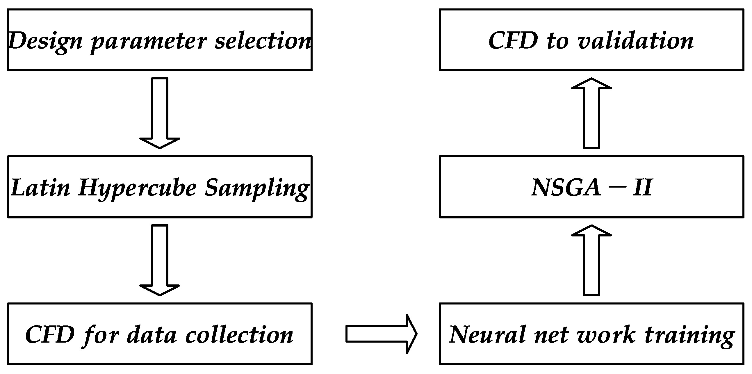
3. Optimization Methods

The overall optimization idea of this study is shown in Figure 6. Firstly, using the structural features of the physical model, we select H, L, and R as our design variables. Subsequently, using the LHS, 50 design points are sampled. The physical model corresponding to the 50 design points is numerically simulated at Re = 1000, and after collecting the numerical simulation data, H, L, and R are used as inputs, and Nu/Nu₀ and f/f₀ are used as outputs to train MLP, where Nu₀ is the Nusselt number of the reference structure and f₀ is the Fanning friction factor of the reference structure. NSGA-II is used to search the design space based on MLP, and after obtaining the Pareto front, the design points with better performance in the Pareto front are selected and reused in the numerical simulation for validation, and the final numerical simulation results are used as the criterion for comparing the performance improvement of the structure.

3.1. Design Parameter Selection and Optimization Problem Formulation

Before completing this optimization process, the input parameters must be identified. In the study by NI et al. [39], it has been verified that the Tesla valve liquid-cooled plate structure without partitions has a superior heat transfer performance and a smaller pressure drop compared to the straight-through channel. The innovative structure proposed in this study is the installation of a partitions at the front end of the Tesla valve to improve the heat transfer and pressure drop performance. This study focuses on the optimization of the geometrical parameters of the partitions. Similarly, the addition of fillet at the fluid convergence may be an important reason for the increase in pressure drop. Therefore, the addition of fillet may also help to improve the pressure drop performance. Accordingly, H, L, and R are selected as the design parameters in this study. The performance differences between different structures at 1000 Reynolds number operating conditions are then investigated.

After determining the design variables and the design variable space, the optimization problem is shown in the following equation:

$$\begin{array}{l}\min (f/f_0)\&\max (Nu/N{u}_0)\\ \left[\begin{array}{c}f/f_0\\ Nu/N{u}_0\end{array}\right]=F(H,R,L)\\ \begin{array}{c}s.t.H\in [0.1,0.4]\\ R\in [0.5,2]\\ L\in [0.5,2]\end{array}\end{array}$$

(14)

where Nu₀ is the Nusselt number of the reference structure and f₀ is the Fanning friction factor of the reference structure. F is an implicit relation constructed by MLP.

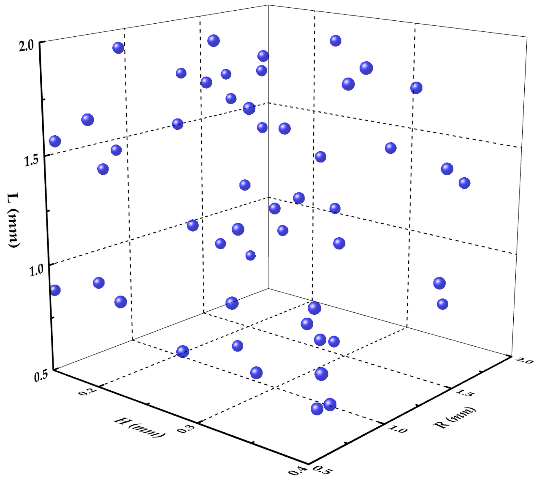
3.2. Design of Experiments

An experimental design approach that minimizes experimental costs by selecting a relatively small number of sample points and maximizes access to information about the experimental design space is an experimental design approach that is worthy of consideration. Classical and modern experimental design methods are both vital and effective strategies for designing experiments. Classical experimental design methods are primarily used for instrumental experiments, whereas modern experimental design methods are utilized for computer experiments. To accurately determine the three design parameters, modern experimental design methods should be used. Latin hypercube sampling (LHS), a modern experimental design method, offers several advantages, including a uniform distribution of sample points, low correlation between dimensions, and ease of implementation. Therefore, the LHS method is the most suitable method for sampling the design parameters in this study.

The basic idea of LHS is to ensure an even distribution of sample points in each dimension, while ensuring that the correlation between sample points between different dimensions is as minimal as possible. Firstly, for each dimension, an equal number of sampling intervals is taken to obtain the same number of small intervals. For example, if you need to sample the interval [a, b] and obain c sample points, you need to divide the interval [a, b] equally into c sub-intervals. Secondly, for each dimension, the sub-intervals need to be rearranged to ensure that each sub-interval contains only one sample point, which ensures that the sampling points in each dimension are evenly distributed. After that, a random position is selected as a sample point in the sub-interval of each dimension, and the above operation is repeated, which ensures that the sample points are evenly distributed and the correlation between the sample points of different dimensions is minimized as much as possible. In this study, MATLAB 2023b was used to implement the LHS.

In light of the structural characteristics and computational complexity of the physical model, this study established the following ranges for the half thickness of the partition H, the length of the partition L, and the radius of the fillet: H is [0.1, 0.4], L is [0.5, 2], and the radius of the fillet is [0.5, 2]. Furthermore, 50 distinct design points were requested to be acquired by LHS within the design space. The results of the sampling are presented in Figure 7. It can be demonstrated that the design points are distributed evenly throughout the design space. This signifies that the selected design points are strategically positioned to illustrate the defining characteristics of the design space in its truest form.

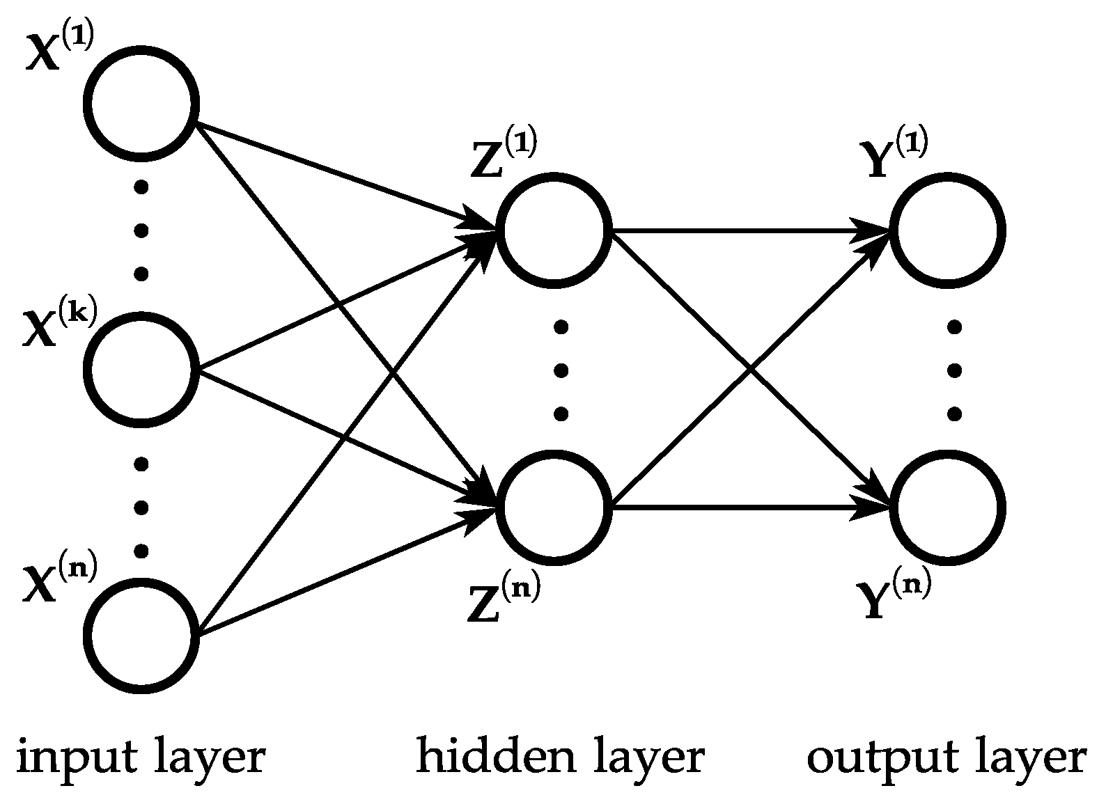
3.3. Neural Network Fitting Model

Neural networks have been widely used for classification tasks or prediction tasks. For the prediction task, it is implemented by fitting an implicit relational equation be-tween input and output using neural networks. MLP refers to a network structure with two layers of neural networks, which is shown in Figure 8. The input layer is responsible for receiving raw data, with each input node corresponding to a feature of the data. For example, if the input data have n features, then the input layer has n nodes. A concealed layer refers to one or more layers in a neural network between the input and output layers. Each concealed layer comprises of multiple neurons (nodes) that connect the concealed layer to the input and output layers through a weight function. Each neuron receives all inputs from the previous layer and outputs a weighted and activation function-processed value. The output layer is responsible for generating the ultimate output of the network, and its number of nodes is generally contingent upon the nature of the problem. For instance, in a prediction problem, the output layer typically has only one node, whereas in a classification problem, the number of nodes in the output layer aligns with the number of possible classes. Equation (14) shows an example computation from the input layer to the concealed layer and Equation (15) shows an example computation from the concealed layer to the output layer:

$$Z^{(1)}=f(W^{(1)}\times X)$$

(15)

$$Y=g(W^{(2)}\times Z^{(1)})$$

(16)

where X is the input data, W⁽¹⁾ is the weight matrix of the concealed layer, and f is the activation function of the concealed layer. W⁽²⁾ is the weight matrix of the output layer, g is the activation function of the output layer. Z⁽¹⁾ is the output of the concealed layer, and Y is the output data.

Prior to neural network training, the LHS has been employed to obtain design points containing as much information as possible within the design space. Consequently, the training results of the neural networks are typically able to perform the prediction task more effectively. Nevertheless, the neural network may still be susceptible to overfitting, necessitating the selection of a training function that minimizes this phenomenon. One such technique is Bayesian regularization backpropagation, a widely employed method for preventing overfitting. Despite an increase in computational complexity, this approach offers several advantages, including a high level of generalization and high prediction accuracy. In this study, MATLAB 2023b is utilized for neural network training. The neural network structure comprises a two-layered feedforward network, with 10 nodes in the concealed layer. The proportion of the training dataset to the validation dataset is 8:2. The training method employs Bayesian regularization backpropagation to minimize the occurrence of overfitting. The number of training rounds is set to 1000.

3.4. Multi-Objective Genetic Algorithm

NSGA-II has been extensively used in the field of parameter optimization. In this study, NSGA-II is employed to identify design points within the design space that exhibit both a low f and a high Nu. Objective variables corresponding to each design point in the design space are obtained from a trained neural network. The search principle of the multi-objective genetic algorithm mimics the inheritance and variation of a population, where a set of vectors used for decision making are analogous to individuals in a population. Each individual represents a possible solution to the problem. A fitness function (objective function) is used to evaluate the degree of excellence of each individual for each objective by constructing a fitness function. In a multi-objective optimization problem, a possible solution is called a Pareto optimal solution, which is the solution that cannot be improved upon and has the best performance on all objectives, and the set of solutions of all Pareto optimal solutions constitutes the Pareto frontier. In this study, we select the design points that may have the best performance based on the Pareto frontier for numerical simulation verification, and determine whether the selected design points have performance improvement through numerical simulation results.

NSGA-II require the initialization of a population with a number of randomly generated individuals in the modified population. In the subsequent process, the first selection is made to retain the individuals that perform better based on Pareto rank or fitness function values, and the selected individuals are used as the next generation of the population. There are two cases in generating the next generation of individuals: (1) crossover is an operation in which the information of two parents is crossed and used to generate new individuals, and (2) mutation is a random change in the genes of an individual that is used to augment the diversity of the population. The above two operations are used to yield new individuals in a continuous cycle to find the Pareto optimal solution. During the iteration process, a non-dominated sorting technique is introduced to maintain the solutions already present in the Pareto front, and the search stops when the iteration reaches the maximum number of iterations or when the convergence of the solutions reaches a predefined condition. In this study, NSGA-II was implemented based on MATLAB R2023b, the Pareto fraction was set to 0.3, the population size was set to 200, the number of generations was set to 300, the number of stopping iterations was set to 1000, and the deviation of the fitness function was set to 1 × 10⁻¹⁰.

4. Results and Analysis

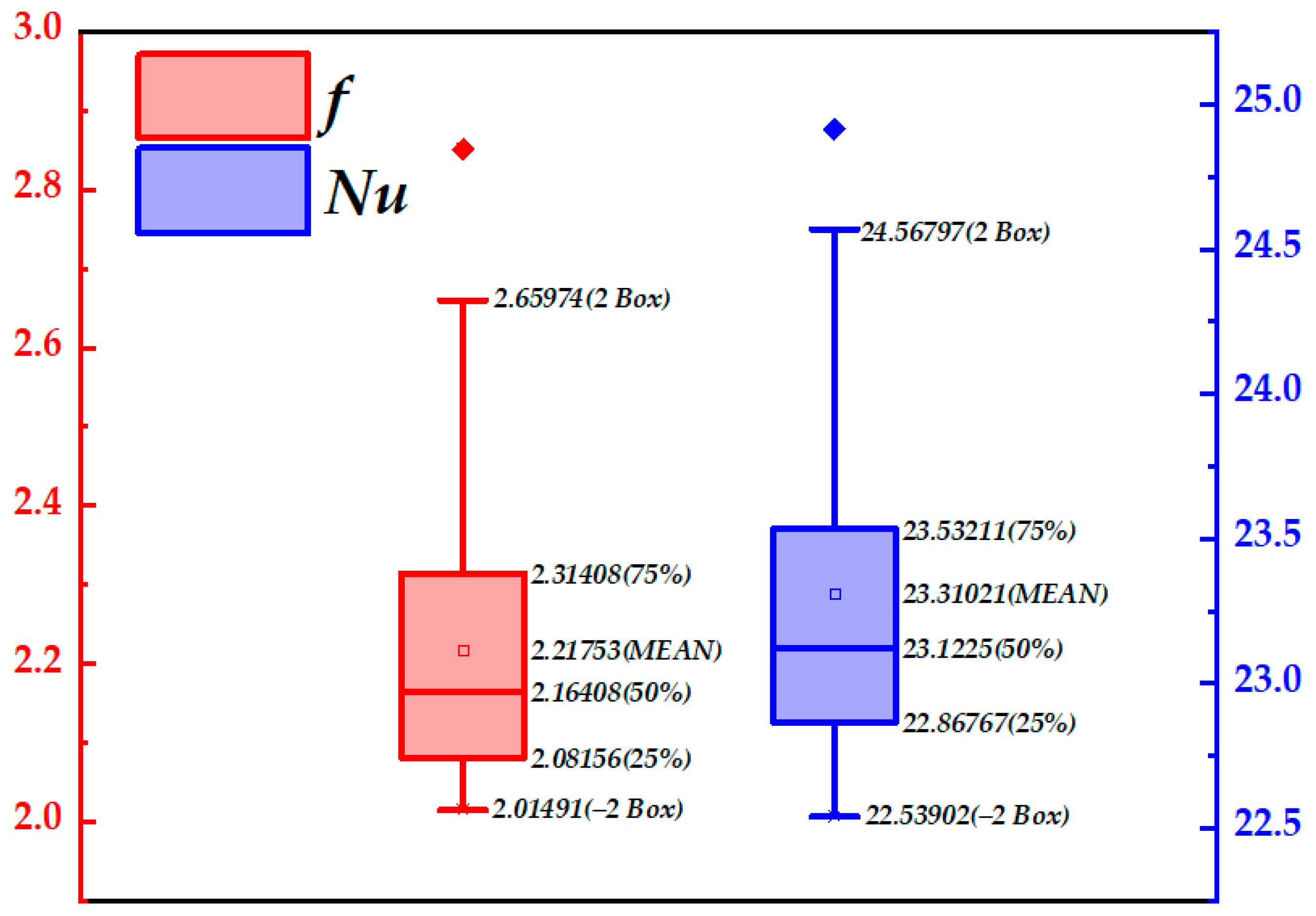
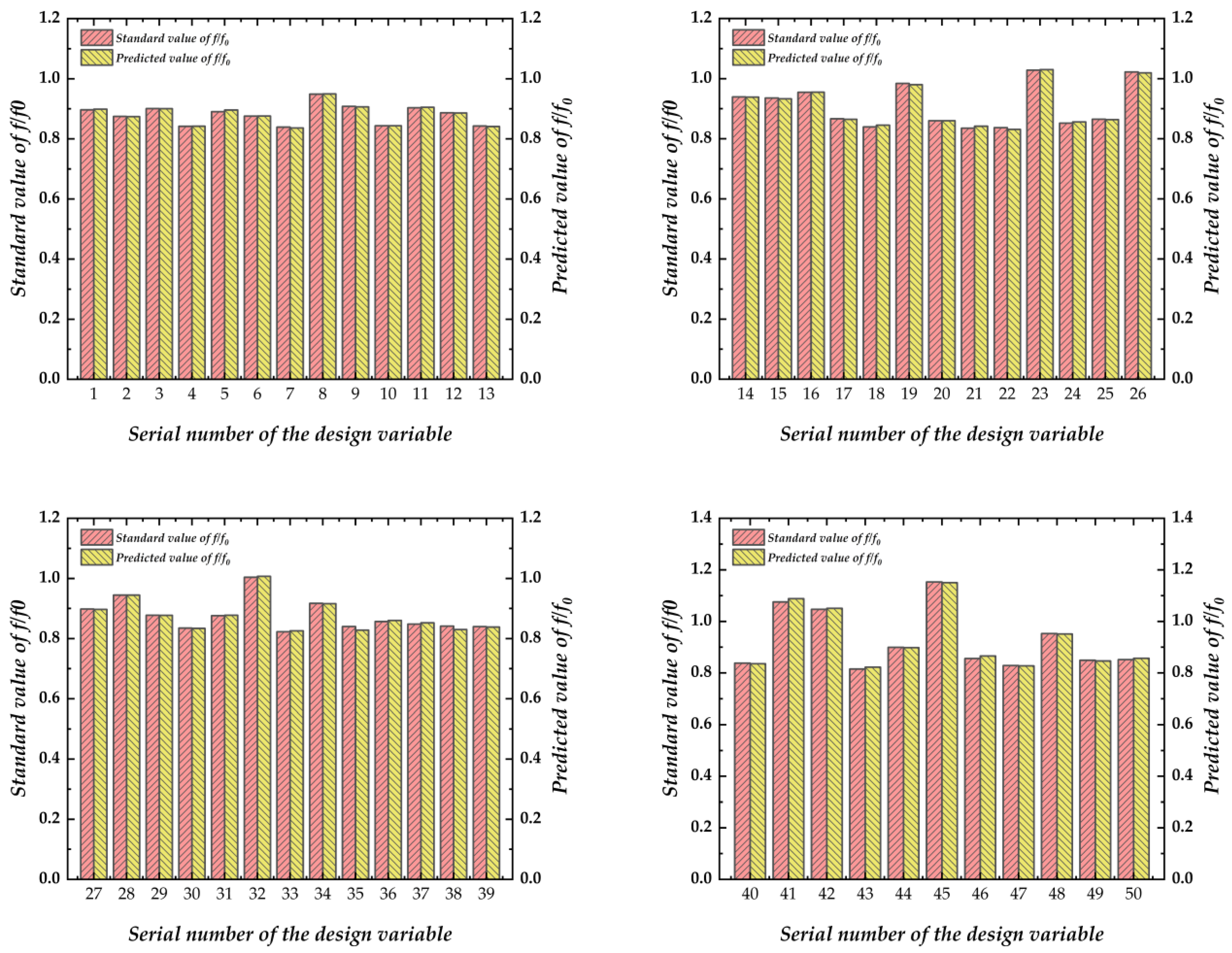
4.1. Dataset Quality Analysis

The quality of the dataset directly affects the veracity of the neural network training results. If the distribution of the target variables in the dataset is not balanced with a greater number of outliers, the neural network may not be able to comprehensively learn the distribution of the corresponding target variables in the design space. This may result in the output of extreme prediction points, which in turn will prevent the subsequent optimization process from being carried out. A high-quality dataset should be free of outliers and exhibit a balanced distribution of target variables.

Outlier detection can be accomplished by plotting a box plot of the target variable. A box plot is a common mathematical and statistical method that employs the minimum, upper quartile, median, lower quartile, and maximum values to describe a statistical graph of data. Box plots permit the visualization of outliers in the data, the dispersion of the data distribution, and the symmetry of the data. The Nu and f, as obtained from numerical simulation, are presented in box plots for the purpose of outlier detection, with the results displayed in Figure 9. For data points exceeding 2 box and falling below −2 box, it can be observed that these are considered outliers. As illustrated in the figure, there is only one outlier for f and only one outlier for Nu. This indicates that the data for the target variables are well distributed and do not appear to deviate significantly from the overall distribution. Once outliers have been identified, a neural network can be trained to establish the implicit relationship between the design and target variables.

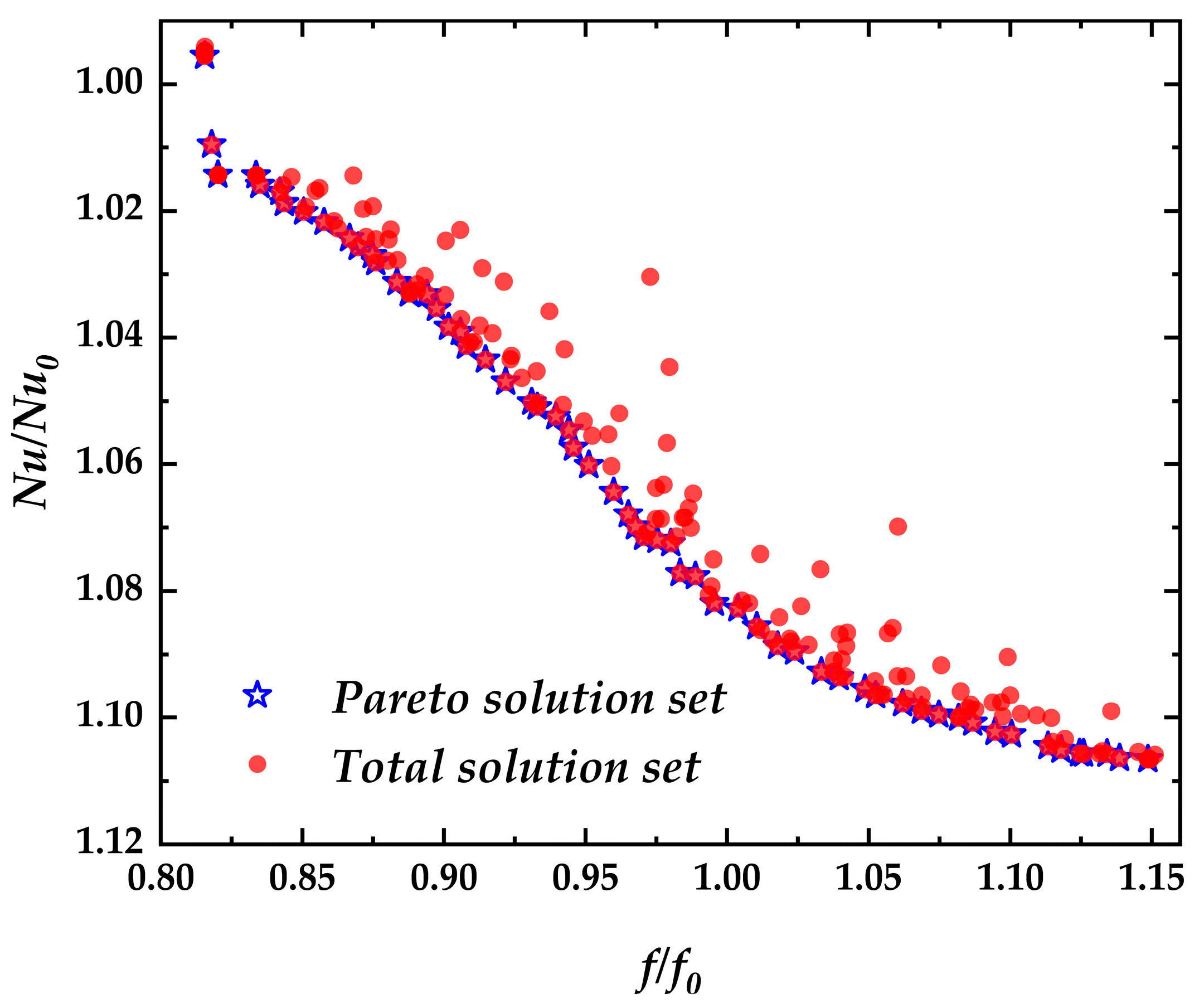
4.2. Optimization Results Analysis

The accuracy of the training results of MLP has a direct impact on the subsequent search accuracy of the NSGA-II. Therefore, it is essential to assess the superiority of the training results of the neural network. In this investigation, MLP is employed to establish the relationship between the input variables and the target variables. The performance of the neural network can be evaluated by utilizing the coefficient of determination, R². R² is an analytical parameter that is employed to assess the predictive ability of a model. The value of R² is constrained between 0 and 1, with a closer proximity to 1 indicating a greater predictive efficacy of the model. The R² can be computed by the following equation:

$$R^2=1-\frac{{{\displaystyle \sum _{i=1}^n(y_i-{\widehat{y}}_i)}}^2}{{{\displaystyle \sum _{i=1}^n(y_i-\overline{y})}}^2}$$

(17)

where the symbol y represents the standard value, the symbol $\widehat{y}$ represents the predicted value, and the symbol $\overline{y}$ represents the mean value.

The predicted and true values of the three design variables were plotted relative to Nu/Nu₀ and f/f₀ for each of the 50 groups. The results are shown in Figure 10 and Figure 11. It can be observed that the discrepancy between the standard value and the true value is minimal, regardless of whether it is Nu/Nu₀ or f/f₀. Furthermore, the maximum error of both variables is maintained below 1%. Furthermore, the R² value for Nu/Nu₀ is equal to 0.9971, while the R² value for f/f₀ is equal to 0.9966. This indicates that the neural network constructed in this study has a high degree of predictive accuracy and is capable of accurately establishing the implicit relationship between the design variables and the two target variables.

Once it has been established that the neural network prediction performance is sufficient for the prediction task, the neural network outputs are employed as inputs to the multi-objective genetic algorithm. The first objective of this algorithm is to maximize Nu/Nu₀, while the second objective is to minimize f/f₀. Once the NSGA-II has conducted its search in the design space, the Pareto frontier is obtained. Figure 12 illustrates the relationship between all solutions and Pareto solutions throughout the design space search. All Pareto solutions collectively constitute the Pareto front, which represents the set of optimal solutions for the two objectives within the design space. The solution with the smallest f/f₀ is considered first, and the solution with the largest Nu/Nu₀ is found on this basis, according to the Pareto front. Based on the aforementioned ideas, the ten sets of solutions that performed the best were identified. To verify the precision of the search, numerical simulations were employed, and the results are presented in

Table 2. Validation of optimization results.

H	R	L	Predicted f/f0	Predicted Nu/Nu0	Standard f/f0	Standard Nu/Nu0	Error f/f0	Error Nu/Nu0
0.250	1.253	0.768	0.836	1.016	0.836	1.009	0.00%	0.69%
0.228	1.285	0.934	0.842	1.017	0.838	1.013	0.48%	0.39%
0.215	1.244	0.995	0.846	1.019	0.843	1.015	0.36%	0.39%
0.222	1.517	1.717	0.957	1.061	0.963	1.061	0.62%	0.00%
0.229	1.619	1.740	0.966	1.064	0.971	1.063	0.51%	0.09%
0.229	1.723	1.760	0.970	1.065	0.975	1.065	0.51%	0.00%
0.236	1.725	1.611	0.940	1.054	0.945	1.052	0.53%	0.19%
0.232	1.492	1.675	0.952	1.059	0.959	1.059	0.73%	0.00%
0.232	1.447	1.631	0.942	1.055	0.949	1.054	0.74%	0.09%
0.234	1.773	1.572	0.930	1.050	0.933	1.048	0.32%	0.19%

. The results of the validated set of 10 design points indicate that there has been a significant improvement in f with respect to the reference structure, with a reduction in the range of 7% to 16%. Additionally, Nu has exhibited a small increase with respect to the reference structure, located in the range of 1% to 6%. The aim of this investigation was to identify a design that minimizes f while maintaining or improving Nu to the greatest extent possible. Consequently, the initial set of design points is deemed the optimal structure for this study. The values of H, R, and L were found to be 0.250, 1.253, and 0.768, respectively. Furthermore, it can be observed that the errors against both target variables are maintained below 1%, which suggests that the accuracy of both the neural network model construction and the multi-objective genetic algorithm search is at a high level. Additionally, the 10 sets of design variables selected are not present in the original dataset. Nevertheless, the prediction outcomes remain highly accurate, indicating that the neural network model effectively minimizes the overfitting phenomenon.

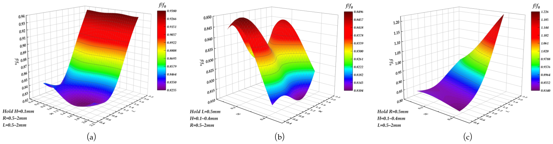
4.3. Parameter Sensitivity Analysis

Once the neural network prediction accuracy and the multi-objective genetic algorithm search accuracy had been verified, it was necessary to ascertain the impact of changes in the three design variables on the target variable. To this end, a parameter sensitivity analysis was performed. The methodology employed in this analysis is based on the control variable method, whereby a single design variable is held constant while the remaining variables are varied in increments of 0.05 mm. All the design variables within a set are inputted into the neural network to obtain the corresponding outputs, thereby exploring the extent to which the varied variables affect the target variables. Figure 13 illustrates the sensitivity analysis outcomes for Nu/Nu₀ and Figure 14 illustrates the sensitivity analysis outcomes for f/f₀. Figure 13a illustrates that Nu/Nu₀ is more responsive to alterations in L when H is maintained constant. Furthermore, Nu/Nu₀ exhibits a notable increase when L is elevated from 1.3 to 2. As L varies across different levels, the impact of the change in R is not uniform. However, the general trend is to increase and then decrease. An observation of Figure 13b reveals that Nu/Nu₀ increases and then decreases as H increases, and Nu/Nu₀ reaches a peak at all levels of R when H is near 0.25. It is when H is located around 0.4 that the change in R exhibits a large effect on Nu/Nu₀. An observation of Figure 13c reveals that the change in L has a significant effect on Nu/Nu₀, showing an increase in Nu/Nu₀ with increasing L at all H levels. Comparison of the three subplots of Figure 13 reveals that the effect of L on Nu/Nu₀ is the most significant, followed by H and finally by R. Figure 14a illustrates that f/f₀ is more responsive to changes in L when H is held constant. As L decreases, f/f₀ tends to remain relatively stable. However, when R is increased, the change in f/f₀ demonstrates an initial increase followed by a decline. At approximately R = 1.3, f/f₀ exhibits a consistent decrease across all levels of L. Figure 14b demonstrates that f/f₀ exhibits an overall increase and subsequent decline as H increases. However, the trend of f/f0 also exhibits a different trend for different levels of R. When R is located near 1.3, f/f₀ is guaranteed to be minimum for all levels of H. This observation is supported by Figure 14c, which reveals that f/f₀ increases significantly with the increase in L, which holds true for H at all levels, indicating that the effect of L on f/f₀ is more significant. A comparison of the subplots of Figure 14 reveals that the largest effect on f/f₀ is exerted by L, followed by H, and finally R. However, it is noteworthy that R at a level of approximately 1.3 significantly reduces f/f₀ for both H and L.

4.4. Comparative Performance Analysis of the Optimal and Reference Structures

To investigate the underlying cause of the performance disparity between the optimal structure and the referenced one, a performance comparison analysis was executed. As shown in Figure 15a, the temperature distribution of the XY plane at a Z value of 5.5 mm is depicted. Figure 15b further demonstrates key pressure distribution features of two structures located at the same position. Figure 15c shows the streamline and velocity distribution of the two structures at the same position. An analysis of Figure 15a shows that due to the addition of partitions, the heat transfer area is increased and the fluid flow capacity is enhanced. The temperature distribution in the first two-thirds of the optimal structured fluid flow area is significantly lower than that of the reference structure. The temperature of the solid part nearest the fluid inlet fluctuates substantially. The lowest temperature observed for the optimal design is 308 K, while the highest is 310 K. In comparison, the same parameters for the reference design are 310 K and 313 K, respectively. The average temperature of the first two-thirds of the solid part also varies. The average temperature of the optimal design is 309.4 K, while the reference design has an average temperature of 311.2 K, resulting in a difference of 1.8 K. In the last third of the fluid flow area, partitions can only affect the flow of a small part of the fluid. Therefore, the temperature distribution of the two structures at the last third is basically the same, which shows that partitions play a role in enhancing heat transfer. However, since Nu represents the cooling capacity after the area is averaged, the Nu of the two structures is not much different. Combined with the analysis of Figure 15b,c, compared to the reference structure, the optimal structure significantly reduces the pressure drop and the vortex phenomenon in the flow field. The difference between the two structures is 160 Pa, with the optimal structure experiencing a 300 Pa pressure drop at the inlet and outlet, while the reference structure experiences a 460 Pa pressure drop. Due to the existence of partitions, the fluid shunt is stable, and the partitions guide the fluid to flow in different directions, greatly reducing the pressure loss caused by the relative movement of the fluid. In the rounded transition section, the fluid near the wall smoothly converges with the fluid in other directions, thereby reducing the occurrence of vortex phenomenon.

The structure shows that the optimized structure significantly reduces the resistance of fluid flow, which is manifested as a smaller pressure drop and a smaller f. Although compared with the reference structure, Nu has little difference on the branches, but the optimized structure has a lower temperature distribution, which shows that the heat dissipation characteristics have also been improved.

5. Conclusions

A multi-objective parameter optimization of liquid-cooled plates with Tesla valves as internal flow paths is conducted using design variables H, R, and L. The objective of the optimization is to maximize Nu and minimize f. Firstly, the Latin oversampling method is employed to oversample the design space. This is then followed by the construction of a neural network prediction model utilizing the simulation data. A multi-objective genetic algorithm is integrated to identify the optimal solution within the design space. Lastly, the optimal structure is selected from the Pareto frontier and verified through simulation. The key findings are as follows:

(1)

The accuracy of the prediction model constructed using the neural network is demonstrably high, with R-squared values of 0.9971 and 0.9966 when the target variable is Nu/Nu₀ and f/f₀, respectively.

(2)

The initial 10 optimal solutions identified by the NSGA-II were found to be highly accurate following simulation validation, with a maximum error of no more than 1% for both objective variables.

(3)

After sensitivity analysis, it is found that L is significant for both target variables, followed by H and finally R. For the design of this structure, smaller values of L and H are recommended, and for R, a value near 1.3 is recommended.

(4)

Compared with the reference structure, the average temperature of the first two-thirds of the solid domain is reduced by 1.8 K, but the temperature of the last one-third of the solid domain is not much different. The inlet and outlet pressure drop of the optimal structure is only 300 Pa, which is reduced by 160 Pa compared with the reference structure.

The introduction of partitions has a minimal impact on Nu, yet it can markedly reduce f. The results of the optimization indicate that the optimal structure exhibits an increase in the Nu of 1% and a reduction in the f of 16% in comparison to the reference structure. Considering the existence of numerical errors, Nu has increased by 1% and f has decreased by 16%, which proves that the designed structure maintains the excellent heat dissipation characteristics inherent in the Tesla valve while significantly reducing the friction resistance and pressure loss of the fluid. This demonstrates the efficacy of the optimization results.

References

1. Akbarzadeh, M.; Jaguemont, J.; Kalogiannis, T.; Karimi, D.; He, J.C.; Jin, L.; Xie, P.; Van Mierlo, J.; Berecibar, M. A novel liquid cooling plate concept for thermal management of lithium-ion batteries in electric vehicles. Energ. Convers. Manag. 2021, 231, 113862. [Google Scholar] [CrossRef]
2. Zhang, X.H.; Li, Z.; Luo, L.A.; Fan, Y.L.; Du, Z.Y. A review on thermal management of lithium-ion batteries for electric vehicles. Energy 2022, 238, 121652. [Google Scholar] [CrossRef]
3. Sheng, L.; Su, L.; Zhang, H.; Li, K.; Fang, Y.D.; Ye, W.; Fang, Y. Numerical investigation on a lithium ion battery thermal management utilizing a serpentine-channel liquid cooling plate exchanger. Int. J. Heat. Mass. Transf. 2019, 141, 658–668. [Google Scholar] [CrossRef]
4. Wu, W.X.; Wang, S.F.; Wu, W.; Chen, K.; Hong, S.H.; Lai, Y.X. A critical review of battery thermal performance and liquid based battery thermal management. Energ. Convers. Manag. 2019, 182, 262–281. [Google Scholar] [CrossRef]
5. Fayaz, H.; Afzal, A.; Samee, A.D.M.; Soudagar, M.E.M.; Akram, N.; Mujtaba, M.A.; Jilte, R.D.; Islam, M.T.; Agbulut, Ü.; Saleel, C.A. Optimization of Thermal and Structural Design in Lithium-Ion Batteries to Obtain Energy Efficient Battery Thermal Management System (BTMS): A Critical Review. Arch. Comput. Methods Eng. 2022, 29, 129–194. [Google Scholar] [CrossRef] [PubMed]
6. Akbarzadeh, M.; Kalogiannis, T.; Jaguemont, J.; Jin, L.; Behi, H.; Karimi, D.; Beheshti, H.; Van Mierlo, J.; Berecibar, M. A comparative study between air cooling and liquid cooling thermal management systems for a high-energy lithium-ion battery module. Appl. Therm. Eng. 2021, 198, 117503. [Google Scholar] [CrossRef]
7. Saechan, P.; Dhuchakallaya, I. Numerical study on the air-cooled thermal management of Lithium-ion battery pack for electrical vehicles. Energy Rep. 2022, 8, 1264–1270. [Google Scholar] [CrossRef]
8. Luo, J.; Zou, D.Q.; Wang, Y.S.; Wang, S.; Huang, L. Battery thermal management systems (BTMs) based on phase change material (PCM): A comprehensive review. Chem. Eng. J. 2022, 430, 132741. [Google Scholar] [CrossRef]
9. Tang, X.W.; Guo, Q.; Li, M.; Wei, C.H.; Pan, Z.Y.; Wang, Y.Q. Performance analysis on liquid-cooled battery thermal management for electric vehicles based on machine learning. J. Power Sources 2021, 494, 229727. [Google Scholar] [CrossRef]
10. Farhan, M.; Amjad, M.; Tahir, Z.U.; Anwar, Z.; Arslan, M.; Mujtaba, A.; Riaz, F.; Imran, S.; Razzaq, L.; Ali, M.; et al. Design and Analysis of Liquid Cooling Plates for Different Flow Channel Configurations. Therm. Sci. 2022, 26, 1463–1475. [Google Scholar] [CrossRef]
11. Jarrett, A.; Kim, I.Y. Design optimization of electric vehicle battery cooling plates for thermal performance. J. Power Sources 2011, 196, 10359–10368. [Google Scholar] [CrossRef]
12. Jarrett, A.; Kim, I.Y. Influence of operating conditions on the optimum design of electric vehicle battery cooling plates. J. Power Sources 2014, 245, 644–655. [Google Scholar] [CrossRef]
13. Jin, L.W.; Lee, P.S.; Kong, X.X.; Fan, Y.; Chou, S.K. Ultra-thin minichannel LCP for EV battery thermal management. Appl. Energ. 2014, 113, 1786–1794. [Google Scholar] [CrossRef]
14. Guo, R.; Li, L. Heat dissipation analysis and optimization of lithium-ion batteries with a novel parallel-spiral serpentine channel liquid cooling plate. Int. J. Heat. Mass. Transf. 2022, 189, 122706. [Google Scholar] [CrossRef]
15. Chen, S.Q.; Peng, X.B.; Bao, N.S.; Garg, A. A comprehensive analysis and optimization process for an integrated liquid cooling plate for a prismatic lithium-ion battery module. Appl. Therm. Eng. 2019, 156, 324–339. [Google Scholar] [CrossRef]
16. Mo, X.B.; Zhi, H.; Xiao, Y.Z.; Hua, H.Y.; He, L. Topology optimization of cooling plates for battery thermal management. Int. J. Heat. Mass. Transf. 2021, 178, 121612. [Google Scholar] [CrossRef]
17. E, J.Q.; Han, D.D.; Qiu, A.; Zhu, H.; Deng, Y.W.; Chen, J.W.; Zhao, X.H.; Zuo, W.; Wang, H.C.; Chen, J.M.; et al. Orthogonal experimental design of liquid-cooling structure on the cooling effect of a liquid-cooled battery thermal management system. Appl. Therm. Eng. 2018, 132, 508–520. [Google Scholar] [CrossRef]
18. Fan, Y.W.; Wang, Z.H.; Fu, T. Multi-objective optimization design of lithium-ion battery liquid cooling plate with double-layered dendritic channels. Appl. Therm. Eng. 2021, 199, 117541. [Google Scholar] [CrossRef]
19. Yuan, J.; Gu, Z.; Bao, J.; Yang, T.; Li, H.; Wang, Y.; Pei, L.; Jiang, H.; Chen, L.; Yuan, C. Structure optimization design and performance analysis of liquid cooling plate for power battery. J. Energy Storage 2024, 87, 111517. [Google Scholar] [CrossRef]
20. Shang, Z.Z.; Qi, H.Z.; Liu, X.T.; Ouyang, C.Z.; Wang, Y.S. Structural optimization of lithium-ion battery for improving thermal performance based on a liquid cooling system. Int. J. Heat. Mass. Transf. 2019, 130, 33–41. [Google Scholar] [CrossRef]
21. Deng, T.; Ran, Y.; Yin, Y.L.; Chen, X.; Liu, P. Multi-objective optimization design of double-layered reverting cooling plate for lithium-ion batteries. Int. J. Heat. Mass. Transf. 2019, 143, 118580. [Google Scholar] [CrossRef]
22. Kudela, J.; Matousek, R. Recent advances and applications of surrogate models for finite element method computations: A review. Soft Comput. 2022, 26, 13709–13733. [Google Scholar] [CrossRef]
23. Gardner, M.W.; Dorling, S.R. Artificial neural networks (the multilayer perceptron)—A review of applications in the atmospheric sciences. Atmos. Environ. 1998, 32, 2627–2636. [Google Scholar] [CrossRef]
24. Kim, K.M.; Hurley, P.; Duarte, J.P. High-resolution prediction of quenching behavior using machine learning based on optical fiber temperature measurement. Int. J. Heat. Mass. Transf. 2022, 184, 122338. [Google Scholar] [CrossRef]
25. Mudawar, I.; Darges, S.J.; Devahdhanush, V.S. Prediction technique for flow boiling heat transfer and critical heat flux in both microgravity and Earth gravity via artificial neural networks (ANNs). Int. J. Heat. Mass. Transf. 2024, 220, 124998. [Google Scholar] [CrossRef]
26. Mann, G.W.; Eckels, S. Multi-objective heat transfer optimization of 2D helical micro-fins using NSGA-II. Int. J. Heat. Mass. Transf. 2019, 132, 1250–1261. [Google Scholar] [CrossRef]
27. Gosselin, L.; Tye-Gingras, M.; Mathieu-Potvin, F. Review of utilization of genetic algorithms in heat transfer problems. Int. J. Heat. Mass. Transf. 2009, 52, 2169–2188. [Google Scholar] [CrossRef]
28. Pan, L.S.; Yao, Z.K.; Yao, W.; Wei, X.L. Multi-objective optimization on bionic fractal structure for heat exchanging of two fluids by genetic algorithm. Int. J. Heat. Mass. Transf. 2023, 212, 124298. [Google Scholar] [CrossRef]
29. Sun, W.; Wen, P.F.; Zhu, S.J.; Zhai, P.C. Geometrical Optimization of Segmented Thermoelectric Generators (TEGs) Based on Neural Network and Multi-Objective Genetic Algorithm. Energies 2024, 17, 2094. [Google Scholar] [CrossRef]
30. Yildizeli, A.; Cadirci, S. Multi objective optimization of a micro-channel heat sink through genetic algorithm. Int. J. Heat. Mass. Transf. 2020, 14, 1188476. [Google Scholar] [CrossRef]
31. Nikola, T. Valvular Conduit. U.S. Patent No. 1,329,559, 3 February 1920. [Google Scholar]
32. Porwal, P.R.; Thompson, S.M.; Walters, D.K.; Jamal, T. Heat transfer and fluid flow characteristics in multistaged Tesla valves. Numer. Heat. Transf. Part. A Appl. 2018, 73, 347–365. [Google Scholar] [CrossRef]
33. Li, K.; Wang, S.; Zong, C.; Liu, Y.; Song, X. Diodicity Optimization of Tesla-Type Check Valve Based on Surrogate Modeling Techniques. In Advances in Mechanical Design; Mechanisms and Machine Science; Springer: Singapore, 2022; pp. 1225–1243. [Google Scholar]
34. de Vries, S.F.; Florea, D.; Homburg, F.G.A.; Frijns, A.J.H. Design and operation of a Tesla-type valve for pulsating heat pipes. Int. J. Heat. Mass. Transf. 2017, 105, 1–11. [Google Scholar] [CrossRef]
35. Monika, K.; Chakraborty, C.; Roy, S.; Sujith, R.; Datta, S.P. A numerical analysis on multi-stage Tesla valve based cold plate for cooling of pouch type Li-ion batteries. Int. J. Heat. Mass. Transf. 2021, 177, 121560. [Google Scholar] [CrossRef]
36. Du, G.; Alsenani, T.R.; Kumar, J.; Alkhalaf, S.; Alkhalifah, T.; Alturise, F.; Almujibah, H.; Znaidia, S.; Deifalla, A. Improving thermal and hydraulic performances through artificial neural networks: An optimization approach for Tesla valve geometrical parameters. Case Stud. Therm. Eng. 2023, 52, 103670. [Google Scholar] [CrossRef]
37. Zhao, Z.; Xu, L.; Gao, J.; Xi, L.; Ruan, Q.; Li, Y. Multi-Objective Optimization of Parameters of Channels with Staggered Frustum of a Cone Based on Response Surface Methodology. Energies 2022, 15, 1240. [Google Scholar] [CrossRef]
38. Zeng, M.; Zhang, G.P.; Li, Y.; Niu, Y.Z.; Ma, Y.; Wang, Q.W. Geometrical Parametric Analysis of Flow and Heat Transfer in the Shell Side of a Spiral-Wound Heat Exchanger. Heat. Transf. Eng. 2015, 36, 790–805. [Google Scholar] [CrossRef]
39. Ni, T.; Si, J.; Li, F.; Pan, C.; Li, D.; Pan, M.; Guan, W. Performance analysis on the liquid cooling plate with the new Tesla valve capillary channel based on the fluid solid coupling simulation. Appl. Therm. Eng. 2023, 232, 120977. [Google Scholar] [CrossRef]
40. Truong, T.Q.; Nguyen, N.T. Simulation and optimization of Tesla valves. Nanotech 2003, 1, 178–181. [Google Scholar]
Figure 1. Physical model of a new liquid-cooled plate with a Tesla valve as an internal channel: (a) an isometric view of physical model; (b) a main view of physical model; (c) a schematic view of physical model; (d) a main view of reference structure.
Energies 17 03106 g001
Figure 2. Isometric view of computational domain.
Energies 17 03106 g002
Figure 3. Main view of computational domain grid partitioning.
Energies 17 03106 g003
Figure 4. Testing grid independence with Nu and pdrop.
Energies 17 03106 g004
Figure 5. Comparison of numerical simulation results and experimental results.
Energies 17 03106 g005
Figure 6. Flow chart of complete multi-objective optimization process.
Energies 17 03106 g006
Figure 7. Sampling distribution of L-H-R parameters using LHS.
Energies 17 03106 g007
Figure 8. Schematic diagram of a typical MLP network structure.
Energies 17 03106 g008
Figure 9. Detecting the outliers of Nu and f in dataset using box plot.
Energies 17 03106 g009
Figure 10. Comparison of differences between predicted value and standard value of Nu/Nu0.
Energies 17 03106 g010
Figure 11. Comparison of differences between predicted value and standard value of f/f0.
Energies 17 03106 g011
Figure 12. Pareto frontiers on Nu/Nu0 and f/f0 obtained by NSGA-II.
Energies 17 03106 g012
Figure 13. Sensitivity analysis of Nu/Nu0 based on MLP: (a) hold H = 0.1 mm, R = 0.5~2 mm, L = 0.5~2 mm; (b) hold L = 0.5 mm, H = 0.1~0.4 mm, R = 0.5~2 mm; (c) hold R = 0.5 mm, H = 0.1~0.4 mm, L = 0.5~2 mm.
Energies 17 03106 g013
Figure 14. Sensitivity analysis of f/f0 based on MLP: (a) hold H = 0.1 mm, R = 0.5~2 mm, L = 0.5~2 mm; (b) hold L = 0.5 mm, H = 0.1~0.4 mm, R = 0.5~2 mm; (c) hold R = 0.5 mm, H = 0.1~0.4 mm, L = 0.5~2 mm.
Energies 17 03106 g014
Figure 15. Performance comparison between optimal structure and reference structure: (a) temperature distribution; (b) pressure distribution; (c) streamline and velocity distribution.
Energies 17 03106 g015