
Application of CFD Simulation to the Design of an Innovative Drying Chamber


Abstract
1. Introduction
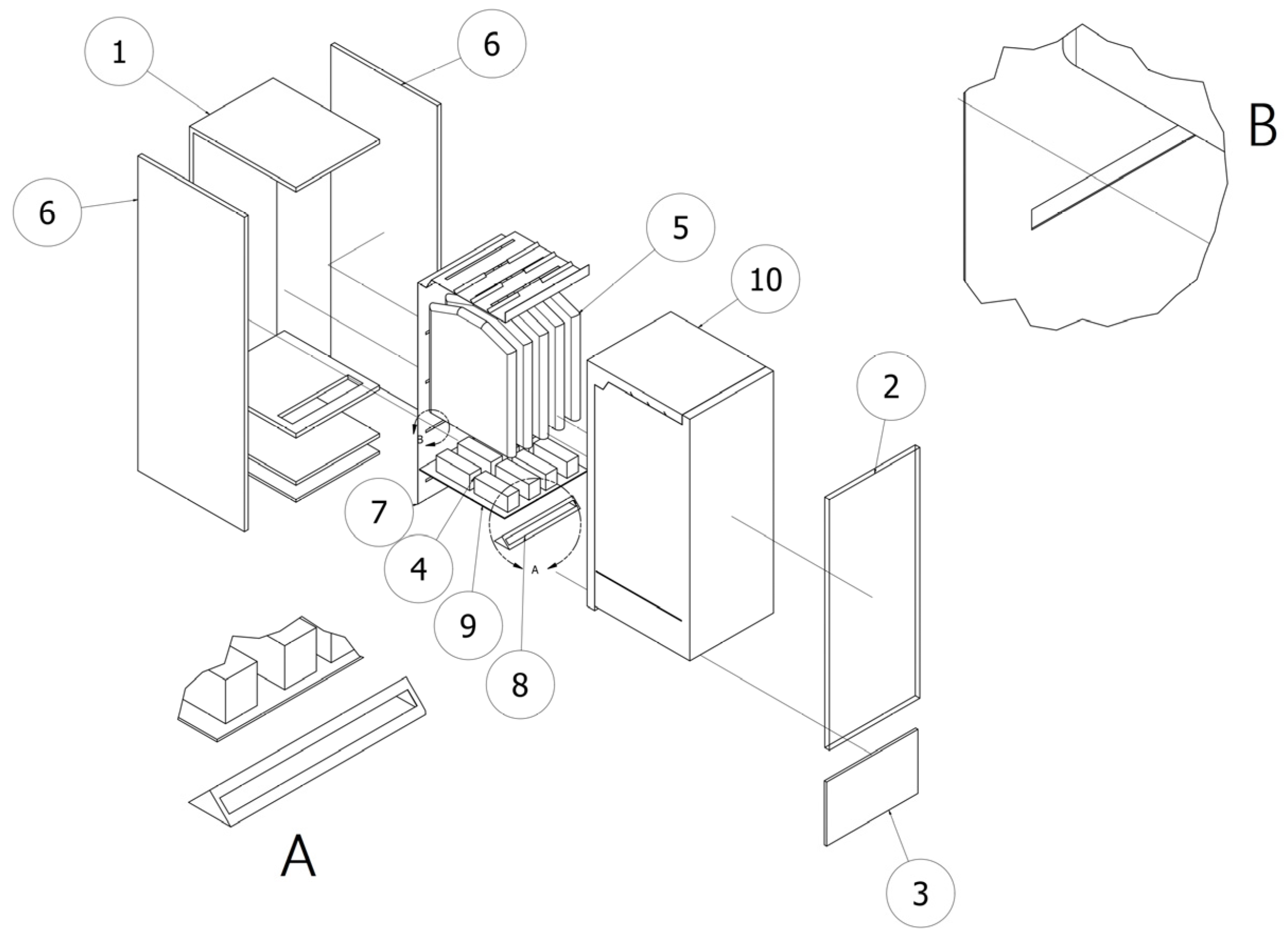
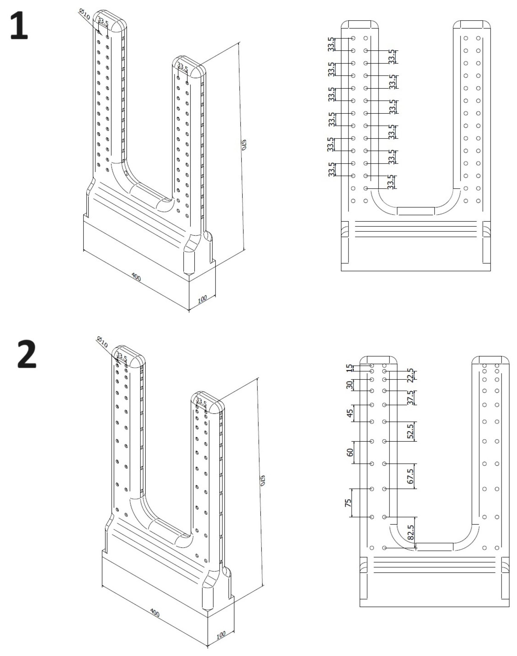
2. Research Subject
3. Simulation Model
- Resolution of the mesh and method of creating cells: linear without mid-side nodes, and quadratic with mid-side nodes. The number of iterations remained constant at 100.
- Gas models: ideal gas, incompressible gas, constant density.
- Iterations of the simulation: 100/500/1000
- Combined simulations: combining simulations with the minimum and maximum number of iterations with the simulation having the highest resolution and the maximum number of mesh elements.
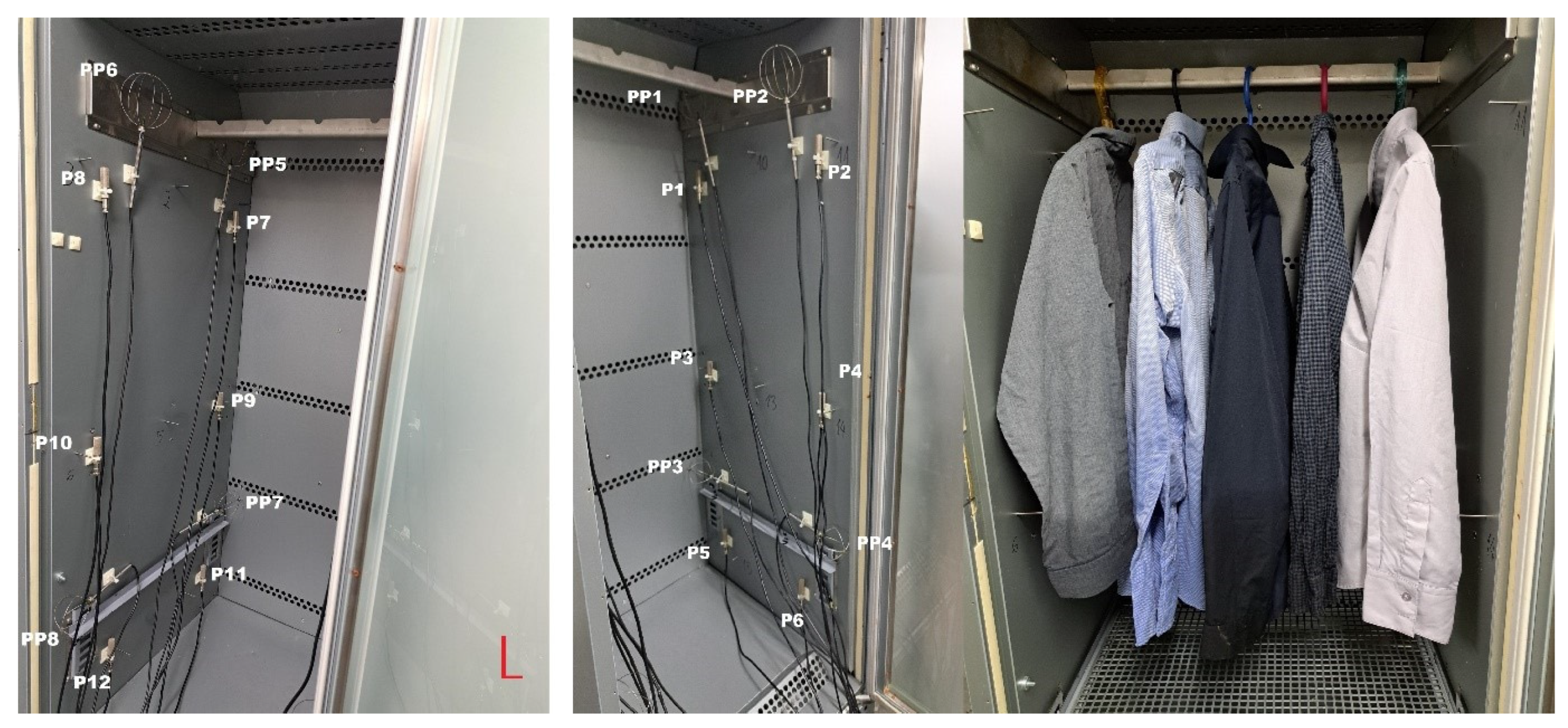
4. Experimental Investigations of the Drying and Sanitising Cabinet
- Air temperature: 25 °C;
- Relative humidity: 60%.
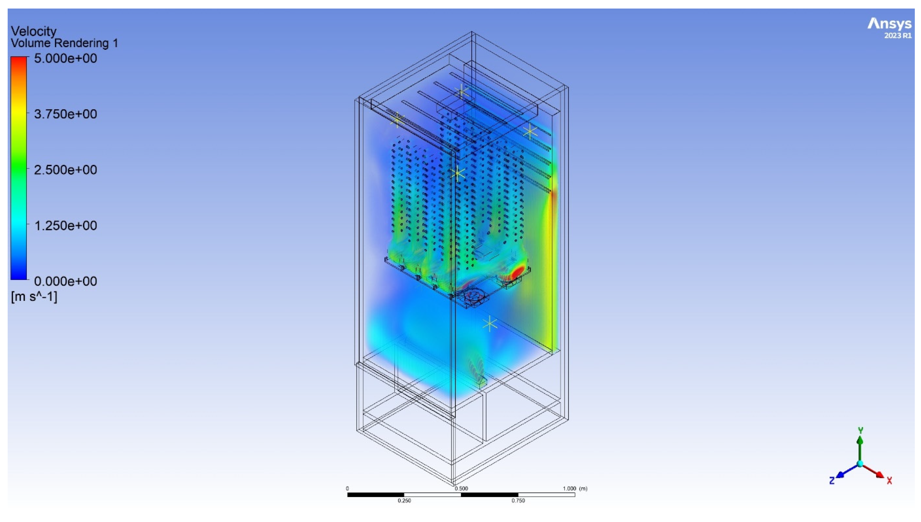
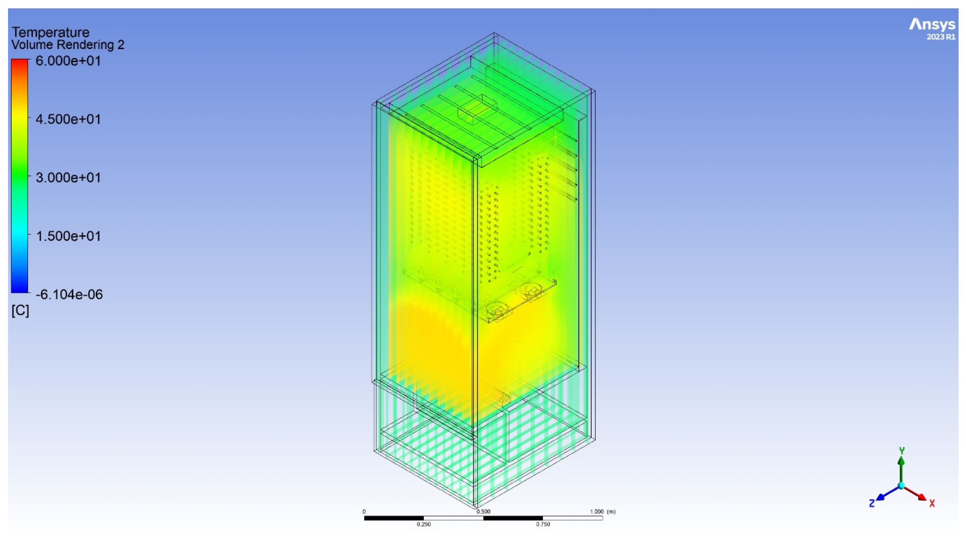
5. Discussion of the Results of the Simulation Model
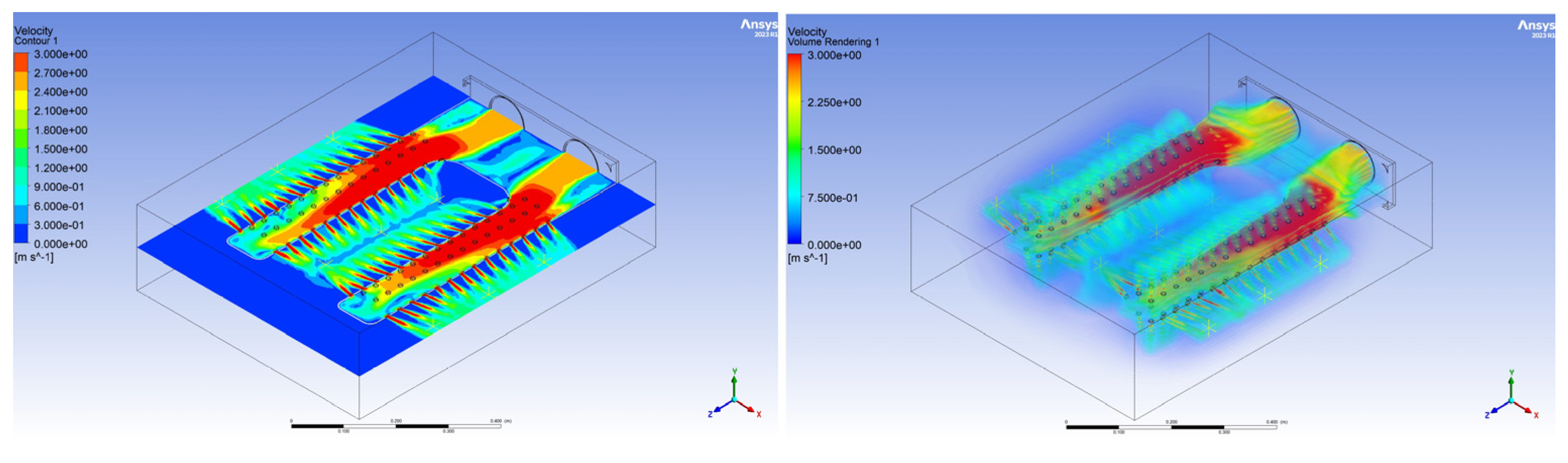
6. The Shape of the Innovative Chamber and Its CFD Optimisation
7. Conclusions
Author Contributions
Funding
Institutional Review Board Statement
Informed Consent Statement
Data Availability Statement
Acknowledgments
Conflicts of Interest
References
- Janusz, S.; Szudarek, M.; Rudniak, L.; Borcuch, M. Analiza parametrów cieplno-przepływowych lamelowego wymiennika ciepła z wykorzystaniem pełnowymiarowego modelu CFD i jego weryfikacji eksperymentalnej. Instal 2022, 6, 29–34. [Google Scholar] [CrossRef]
- Stribling, D. Investigation into the Design and Optimisation of Multideck Refrigerated Display Cases. Ph.D. Thesis, Department of Mechanical Engineering, Brunel University, Uxbridge, UK, 1997. Available online: https://api.semanticscholar.org/CorpusID:107707490 (accessed on 13 November 2023).
- Mołczan, T.; Cyklis, P. Impact of the Evaporation Temperature on the Air-Drying Rate for a Finned Heat Exchanger. Energies 2023, 16, 2132. [Google Scholar] [CrossRef]
- Ryu, J.-B.; Jung, C.-Y.; Yi, S.-C. Three-dimensional simulation of the humid-air dryer using computational fluid dynamics. J. Ind. Eng. Chem. 2013, 19, 1092–1098. [Google Scholar] [CrossRef]
- Al-Kayiem, H.H.; Gitan, A.A. Flow uniformity assessment in a multi-chamber cabinet of a hybrid solar dryer. Sol. Energy 2021, 224, 823–832. [Google Scholar] [CrossRef]
- Dasore, A.; Konijeti, R. Numerical Simulation of air Temperature and airflow Distribution in a Cabinet tray Dryer. Int. J. Innov. Technol. Explor. Eng. 2019, 8, 1836–1840. [Google Scholar] [CrossRef]
- Pintanaa, P.; Thanompongchart, P.; Phimphilai, K.; Tippayawong, N. Improvement of Airflow Distribution in a Glutinous Rice Cracker Drying Cabinet. Energy Procedia 2017, 138, 325–330. [Google Scholar] [CrossRef]
- Sun, J.; Tsamos, K.M.; Tassou, S.A. CFD comparisons of open-type refrigerated display cabinets with/without air guiding strips. Energy Procedia 2017, 123, 54–61. [Google Scholar] [CrossRef]
- Titariya, V.K.; Tiwari, A.C. Parametric Investigation of the Air Curtain for Open Refrigerated Display Cabinets. Int. J. Soft Comput. Eng. 2012, 2, 121–126. [Google Scholar]
- Ambarita, H.; Nasution, A.H.; Siahaan, N.M.; Kawai, H. Performance of a clothes drying cabinet by utilizing waste heat from a split-type residential air conditioner. Case Stud. Therm. Eng. 2016, 8, 105–114. [Google Scholar] [CrossRef]
- Zhao, H.-B.; Wu, K.; Zhang, J.-F. Simulation Study on Active Air Flow Distribution Characteristics of Closed Heat Pump Drying System with Waste Heat Recovery. Energies 2021, 14, 6358. [Google Scholar] [CrossRef]
- Wang, D.; Tan, L.; Yuan, Y.; Lu, Y. CFD simulation and optimization on airflow uniformity of material drying room used in steam blanching and hot-air vacuum drying equipment. J. Mech. Sci. Technol. 2023, 37, 5463–5474. [Google Scholar] [CrossRef]
- K-Epsilon Turbulence Models. Available online: https://www.simscale.com/docs/simulation-setup/global-settings/k-epsilon/ (accessed on 13 November 2023).
- Reid, K.E. Numerical Simulation Using Transition SST Model to Analyze Effects of Expanding. Manifold Angle and Jet Spacing for Submerged Liquid Jet Impingement. Ph.D. Thesis, Auburn University, Auburn, AL, USA, 2018. Available online: http://hdl.handle.net/10415/6330 (accessed on 13 November 2023).


| Drying method | R290 heat pump |
| Disinfection method | Ozonation (400 mg/h) |
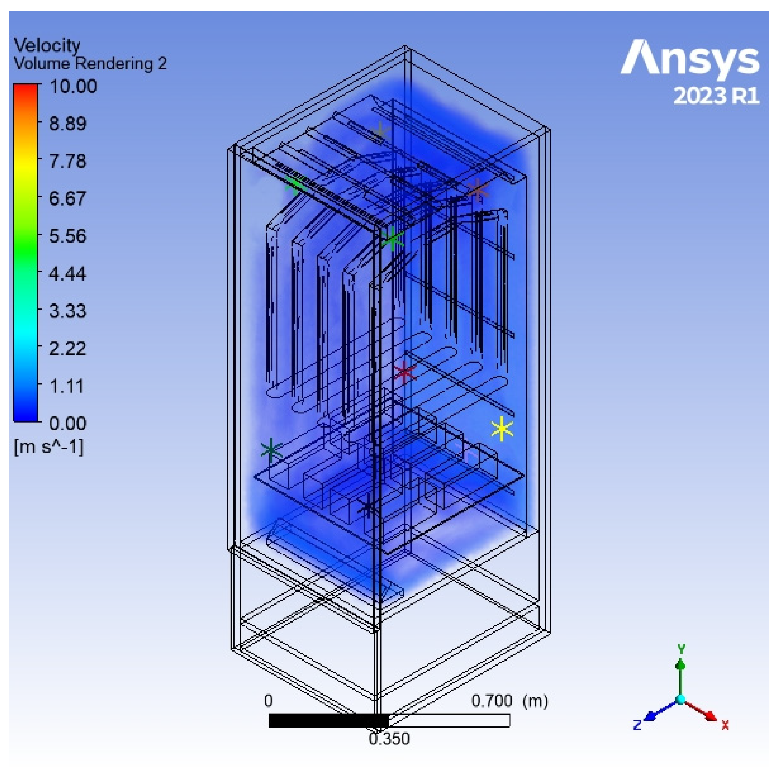
| External dimensions: width/depth/height | 600/735/2000 mm |
| Internal volume | 0.8 m3 |
| Temperature range | 35 to 45 °C |
| Electric power | 700 W |
| Rated current | 5.0 A |
| The velocity of airflow at the inlet of the perforation channel, considering the heat pump | 1.1 m/s |
| Static relative pressure at the inlet of the perforation channel, considering the heat pump. | 0 Pa |
| Intensity of turbulence | 5% |
| Velocity coefficient of turbulence | 10 |
| Inlet air temperature | 40 °C |
| Heat transfer coefficient for insulated walls of thedevice | 0.88 |
| Heat transfer coefficient for the glass doors of the device | 5.7 |
| Heat transfer coefficient of heat transfer for the sheet metal panels | 21.25 |
| Airflow Probe HD103T | |
|---|---|
| Measurement range of airflow | 0.1–5 (m/s) |
| Accuracy of airflow velocity measurements | ±0.1 m/s in the range 0–0.99 m/s, ±0.4 m/s in the range 1.00–5.00 m/s (at 50% RH and 1013 hPa) |
| Type J thermocouple temperature sensor, Class 2 | |
| Measurement range of temperature | +20–+750 °C |
| Accuracy of temperature measurements | ±2.5 °C, Class 2 |
| Humidity sensor (SHT030) | |
| Measurement range of humidity | 0 to 100% RH |
| Accuracy of humidity measurements | 0.2% RH |
| Datalogger (Comet MS6D) | |
| Operating temperature | 0 to +50 °C |
| Channels | 1 to 16 inputs—software configurable |
| Memory | 2 MB (up to 480,000 values) |
| Memory type | Internal SRAM, backed up by a lithium battery |
| Recording interval | Adjustable individually for all input channels from 1 s to 24 h |
| Recording interval | Noncyclic (data-logging stops after filling the memory), Cyclic (after filling the memory, oldest data are overwritten by new) |
| Resolution of the AD converter (analogue channels) | 16 bits; duration of conversion, approximately 60 ms/channel |
| Communication speed | 9600/19,200/57,600/115,200 Bd/ 230,400 * Bd |
| Communication protocol | www, XML, SNMP, SOAP, Modbus TCP |
| Power | 24 Vdc |
| Analog signal converter (MaxMod Ax) | |
| Number of analogue channels | 16 |
| Measurement ranges | Selectable in the ordering stage (−10 to 10 V, 0–10 V, 0–20 mA, or 4–20 mA) |
| Resolution | 16-bit (for a −10 to 10 V signal), 15-bit (for 0–10 V, 0–20 mA, or 4–20 mA signals) |
| Maximum measurement frequency | Up to 1 kHz (simultaneously on 15 measurement channels, for 16 measurement channels, the maximum frequency was 500 Hz) |
| Interface | USB, RS-485 (Modbus RTU) |
| Power supply | 8–33 V DC |
| Arduino Mega 2560 Rev3—A000067 | |
| Number of analogue channels | 16 |
| Number of digital channels | 56 |
| Power | 7 to 12 Vdc |
| Memory | 256 kB |
| Interface | USB |
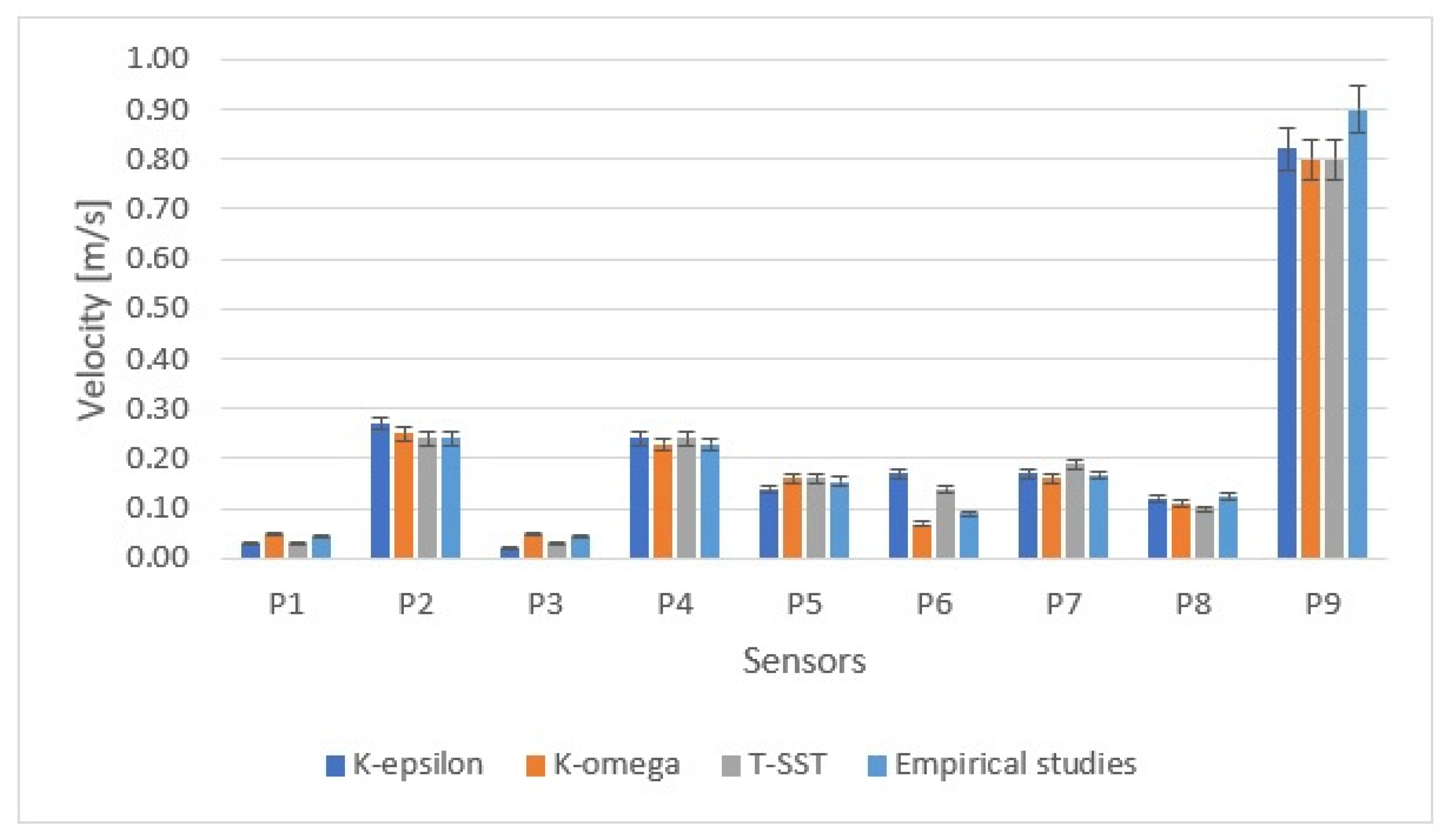
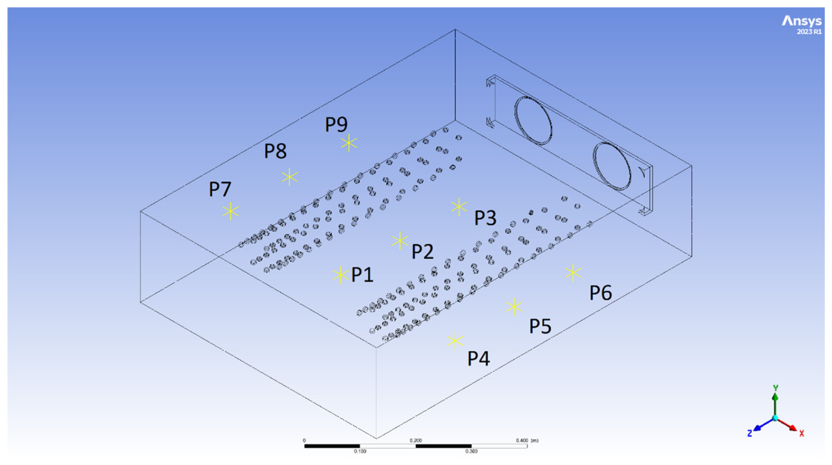
| Measurement Point | Point 1 (PP3) | Point 2 (PP4) | Point 3 (PP7) | Point 4 (PP8) | Point 5 (PP1) | Point 6 (PP2) | Point 7 (PP5) | Point 8 (PP6) | Point 9 (PP9) |
|---|---|---|---|---|---|---|---|---|---|
| Average velocity (m/s) | 0.044 | 0.24 | 0.043 | 0.23 | 0.155 | 0.09 | 0.167 | 0.124 | 0.9 |
| Turbulence Model | ||||||||||
|---|---|---|---|---|---|---|---|---|---|---|
| K-Epsilon | K-Omega | T-SST | K-Epsilon | K-Omega | T-SST | K-Epsilon | K-Omega | T-SST | ||
| Number of iterations | 100 | 100 | 100 | 500 | 500 | 500 | 1000 | 1000 | 1000 | |
| Air velocity (m/s) | P1 | 16.00 | 0.09 | 0.67 | 57.17 | 9.94 | - | 42.97 | 47.05 | - |
| P2 | 9.76 | 0.13 | 0.77 | 42.93 | 12.47 | - | 97.34 | 37.66 | - | |
| P3 | 36.04 | 0.15 | 0.39 | 37.37 | 7.79 | - | 88.84 | 52.50 | - | |
| P4 | 11.01 | 0.24 | 1.08 | 23.55 | 12.56 | - | 64.53 | 77.67 | - | |
| P5 | 346.97 | 0.10 | 0.63 | 98.16 | 3.22 | - | 90.14 | 38.89 | - | |
| P6 | 336.76 | 0.13 | 0.60 | 60.34 | 4.97 | - | 89.29 | 35.80 | - | |
| P7 | 158.50 | 0.19 | 0.39 | 53.16 | 4.12 | - | 81.07 | 15.56 | - | |
| P8 | 202.53 | 0.04 | 0.22 | 100.31 | 3.36 | - | 77.87 | 22.60 | - | |
| P9 | 34.60 | 0.70 | 1.07 | 76.12 | 12.53 | - | 114.34 | 122.34 | - | |
| Test time (hh:mm:ss) | 00:01:42 | 00:02:10 | 00:02:25 | 00:06:09 | 00:07:40 | - | 00:12:14 | 00:14:29 | - | |
| Turbulence Model | ||||||||||
|---|---|---|---|---|---|---|---|---|---|---|
| K-Epsilon | K-Omega | T-SST | K-Epsilon | K-Omega | T-SST | K-Epsilon | K-Omega | T-SST | ||
| Number of iterations | 100 | 100 | 100 | 100 | 100 | 100 | 100 | 100 | 100 | |
| Air velocity (m/s) | P1 | 16.00 | 0.09 | 0.67 | 8.30 | 0.10 | 0.08 | 0.03 | 0.05 | 0.03 |
| P2 | 9.76 | 0.13 | 0.77 | 10.80 | 0.28 | 0.24 | 0.27 | 0.25 | 0.24 | |
| P3 | 36.04 | 0.15 | 0.39 | 23.18 | 0.09 | 0.08 | 0.02 | 0.05 | 0.03 | |
| P4 | 11.01 | 0.24 | 1.08 | 10.91 | 0.31 | 0.26 | 0.24 | 0.23 | 0.24 | |
| P5 | 346.97 | 0.10 | 0.63 | 8.82 | 0.16 | 0.16 | 0.14 | 0.16 | 0.16 | |
| P6 | 336.76 | 0.13 | 0.60 | 4.04 | 0.12 | 0.08 | 0.17 | 0.07 | 0.14 | |
| P7 | 158.50 | 0.19 | 0.39 | 12.11 | 0.11 | 0.12 | 0.17 | 0.16 | 0.19 | |
| P8 | 202.53 | 0.04 | 0.22 | 8.86 | 0.07 | 0.04 | 0.12 | 0.11 | 0.10 | |
| P9 | 34.60 | 0.70 | 1.07 | 2.30 | 0.61 | 0.64 | 0.82 | 0.80 | 0.80 | |
| Test time (hh:mm:ss) | 00:01:42 | 00:02:10 | 00:02:25 | 9 min, 11 s | 7 min, 58 s | 10 min, 30 s | 33 min, 59 s | 37 min, 7 s | 47 min, 58 s | |
| Mesh | Order of elements | Linear | Linear | Linear | Linear | Linear | Linear | Linear | Linear | Linear |
| Resolution | 2 | 2 | 2 | 4 | 4 | 4 | 7 | 7 | 7 | |
| Nodes | 21,524 | 21,524 | 21,524 | 126,034 | 126,034 | 126,034 | 350,622 | 350,622 | 350,622 | |
| Elements | 76,298 | 76,298 | 76,298 | 439,193 | 439,193 | 439,193 | 1,583,065 | 1,583,065 | 1,583,065 | |
| Turbulence model | ||||||||||
| K-epsilon | K-omega | T-SST | K-epsilon | K-omega | T-SST | |||||
| Number of iterations | 100 | 100 | 100 | 100 | 100 | 100 | ||||
| Air velocity (m/s) | P1 | 0.05 | 0.03 | 0.03 | 0.02 | 0.04 | 0.03 | |||
| P2 | 0.26 | 0.27 | 0.26 | 0.25 | 0.24 | 0.25 | ||||
| P3 | 0.04 | 0.04 | 0.03 | 0.03 | 0.04 | 0.01 | ||||
| P4 | 0.27 | 0.26 | 0.25 | 0.25 | 0.23 | 0.23 | ||||
| P5 | 0.14 | 0.17 | 0.17 | 0.16 | 0.18 | 0.18 | ||||
| P6 | 0.2 | 0.17 | 0.14 | 0.1 | 0.16 | 0.17 | ||||
| P7 | 0.15 | 0.14 | 0.15 | 0.16 | 0.12 | 0.15 | ||||
| P8 | 0.09 | 0.1 | 0.1 | 0.12 | 0.21 | 0.2 | ||||
| P9 | 0.78 | 0.78 | 0.78 | 0.8 | 0.79 | 0.79 | ||||
| Test time (hh:mm:ss) | 00:12:41 | 00:13:26 | 00:17:15 | 00:28:26 | 00:32:23 | 00:38:09 | ||||
| Mesh | Order of elements | Quadratic | Quadratic | Quadratic | Quadratic | Quadratic | Quadratic | |||
| Resolution | 5 | 5 | 5 | 6 | 6 | 6 | ||||
| Nodes | 984,686 | 984,686 | 984,686 | 3,227,113 | 3,227,113 | 3,227,113 | ||||
| Elements | 633,908 | 633,908 | 633,908 | 1,737,174 | 1,737,174 | 1,737,174 | ||||
| Turbulence Model | |||||||
|---|---|---|---|---|---|---|---|
| K-Epsilon | K-Omega | T-SST | K-Epsilon | K-Omega | T-SST | ||
| Number of iterations | 100 | 100 | 100 | 1000 | 1000 | 1000 | |
| Air velocity (m/s) | P1 | 0.03 | 0.05 | 0.03 | 0.03 | 0.03 | 0.03 |
| P2 | 0.27 | 0.25 | 0.24 | 0.27 | 0.24 | 0.24 | |
| P3 | 0.02 | 0.05 | 0.03 | 0.03 | 0.04 | 0.05 | |
| P4 | 0.24 | 0.23 | 0.24 | 0.24 | 0.24 | 0.24 | |
| P5 | 0.14 | 0.16 | 0.16 | 0.15 | 0.15 | 0.16 | |
| P6 | 0.17 | 0.07 | 0.14 | 0.18 | 0.06 | 0.17 | |
| P7 | 0.17 | 0.16 | 0.19 | 0.18 | 0.17 | 0.19 | |
| P8 | 0.12 | 0.11 | 0.10 | 0.14 | 0.16 | 0.09 | |
| P9 | 0.82 | 0.80 | 0.80 | 0.82 | 0.81 | 0.80 | |
| Test time (hh:mm:ss) | 00:33:59 | 00:37:07 | 00:47:58 | 05:11:56 | 06:11:12 | 07:18:46 | |
| Mesh | Order of elements | 7 | 7 | 7 | 7 | 7 | 7 |
| Nodes | 350,622 | 350,622 | 350,622 | 350,622 | 350,622 | 350,622 | |
| Elements | 1,583,065 | 1,583,065 | 1,583,065 | 1,583,065 | 1,583,065 | 1,583,065 | |
| Turbulence Model | |||||||
|---|---|---|---|---|---|---|---|
| K-Epsilon | K-Omega | T-SST | K-Epsilon | K-Omega | T-SST | ||
| Number of iterations | 100 | 100 | 100 | 100 | 100 | 100 | |
| Air velocity (m/s) | P1 | 0.02 | 0.04 | 0.03 | 0.02 | 0.04 | 0.02 |
| P2 | 0.25 | 0.24 | 0.25 | 0.25 | 0.24 | 0.25 | |
| P3 | 0.03 | 0.04 | 0.01 | 0.03 | 0.03 | 0.01 | |
| P4 | 0.25 | 0.23 | 0.23 | 0.25 | 0.23 | 0.22 | |
| P5 | 0.16 | 0.18 | 0.18 | 0.16 | 0.18 | 0.18 | |
| P6 | 0.1 | 0.16 | 0.17 | 0.10 | 0.17 | 0.19 | |
| P7 | 0.16 | 0.12 | 0.15 | 0.16 | 0.14 | 0.14 | |
| P8 | 0.12 | 0.21 | 0.2 | 0.13 | 0.22 | 0.22 | |
| P9 | 0.8 | 0.79 | 0.79 | 0.80 | 0.79 | 0.79 | |
| Test time (hh:mm:ss) | 00:28:26 | 00:32:23 | 00:38:09 | 00:27:45 | 00:31:49 | 00:37:39 | |
| Mesh | Order of elements | Quadratic | Quadratic | Quadratic | Quadratic | Quadratic | Quadratic |
| Resolution | 6 | 6 | 6 | 6 | 6 | 6 | |
| Nodes | 3,227,113 | 3,227,113 | 3,227,113 | 3,227,113 | 3,227,113 | 3,227,113 | |
| Elements | 1,737,174 | 1,737,174 | 1,737,174 | 1,737,174 | 1,737,174 | 1,737,174 | |
| Fluid model | Constant density | Constant density | Constant density | Ideal gas | Ideal gas | Ideal gas | |
| Turbulence Model | |||||||
|---|---|---|---|---|---|---|---|
| K-Epsilon | K-Omega | T-SST | K-Epsilon | K-Omega | T-SST | ||
| Number of iterations | 100 | 100 | 100 | 100 | 100 | 100 | |
| Air velocity (m/s) | P1 | 0.02 | 0.04 | 0.02 | 0.02 | 0.04 | 0.02 |
| P2 | 0.25 | 0.24 | 0.25 | 0.25 | 0.24 | 0.25 | |
| P3 | 0.03 | 0.03 | 0.01 | 0.03 | 0.03 | 0.01 | |
| P4 | 0.25 | 0.23 | 0.22 | 0.25 | 0.22 | 0.22 | |
| P5 | 0.16 | 0.18 | 0.18 | 0.16 | 0.18 | 0.18 | |
| P6 | 0.10 | 0.17 | 0.19 | 0.10 | 0.16 | 0.18 | |
| P7 | 0.16 | 0.14 | 0.14 | 0.16 | 0.13 | 0.14 | |
| P8 | 0.13 | 0.22 | 0.22 | 0.13 | 0.22 | 0.22 | |
| P9 | 0.80 | 0.79 | 0.79 | 0.80 | 0.79 | 0.79 | |
| Test time (hh:mm:ss) | 00:27:45 | 00:31:49 | 00:37:39 | 00:26:22 | 00:28:44 | 00:34:58 | |
| Mesh | Order of elements | Quadratic | Quadratic | Quadratic | Quadratic | Quadratic | Quadratic |
| Resolution | 6 | 6 | 6 | 6 | 6 | 6 | |
| Nodes | 3,227,113 | 3,227,113 | 3,227,113 | 3,227,113 | 3,227,113 | 3,227,113 | |
| Elements | 1,737,174 | 1,737,174 | 1,737,174 | 1,737,174 | 1,737,174 | 1,737,174 | |
| Fluid model | Ideal gas | Ideal gas | Ideal gas | Ideal gas + incompressible | Ideal gas + incompressible | Ideal gas + incompressible | |
| Turbulence model | K-omega |
| Simulation method | Coupled |
| Number of iterations | 100 |
| Resolution level | 7 |
| Cell creation | Linear |
| Gas model | Constant density |
| Air velocity at the inlet of the duct inlet at the fan’s location | 2.6 m/s |
| Relative pressure at the inlet of the perforation channel at the heat pump | 0 Pa |
| Intensity of turbulence | 5% |
| Turbulence–velocity ratio | 10 |
| Turbulence model | K-omega SST |
| Simulation method | Coupled |
| Number of iterations | 100 |
| Version 1 | Version 2 | ||
|---|---|---|---|
| Air velocity (m/s) | P1 | 0.55 | 0.37 |
| P2 | 0.50 | 0.46 | |
| P3 | 0.67 | 0.6 | |
| P4 | 0.74 | 1.45 | |
| P5 | 0.62 | 0.22 | |
| P6 | 0.66 | 0.56 | |
| P7 | 0.69 | 1.56 | |
| P8 | 0.65 | 0.28 | |
| P9 | 0.64 | 0.67 | |
| Order of elements | Linear | Linear | |
| Resolution | 7 | 7 | |
| Nodes | 477,174 | 429,215 | |
| Elements | 2,568,181 | 2,306,066 |
| Measurement Point | P1 | P2 | P3 | P4 | P5 | P6 | P7 | P8 |
|---|---|---|---|---|---|---|---|---|
| Average velocity (m/s), simulation | 0.68 | 4.45 | 0.73 | 4.46 | 0.25 | 0.12 | 0.24 | 0.11 |
| Average velocity (m/s), experimental measurement | 0.69 | 4.49 | 0.70 | 4.44 | 0.22 | 0.11 | 0.22 | 0.10 |
| Measurement error % | 1.5 | 0.9 | 4.2 | 0.4 | 12.8 | 8.7 | 8.7 | 9.5 |
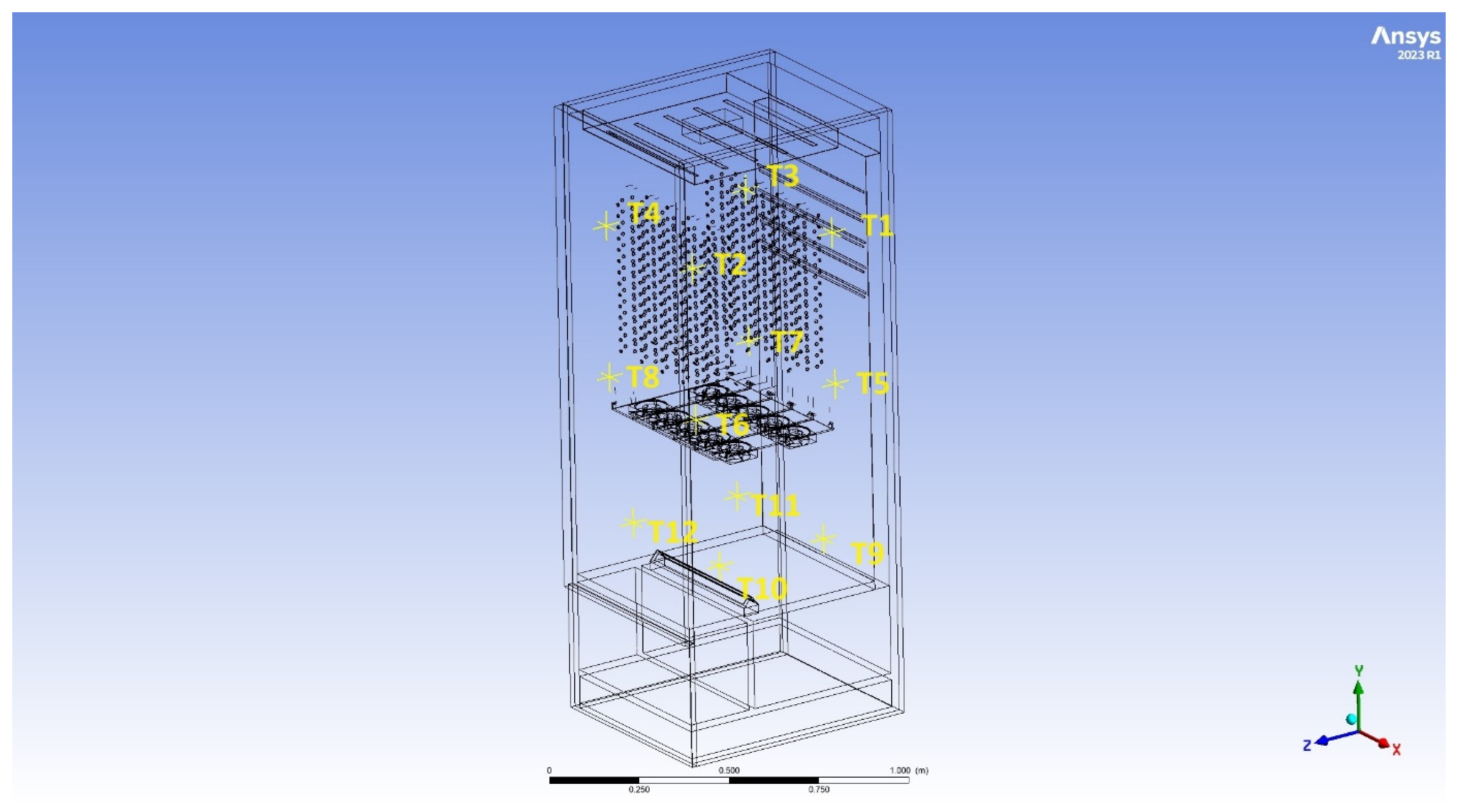
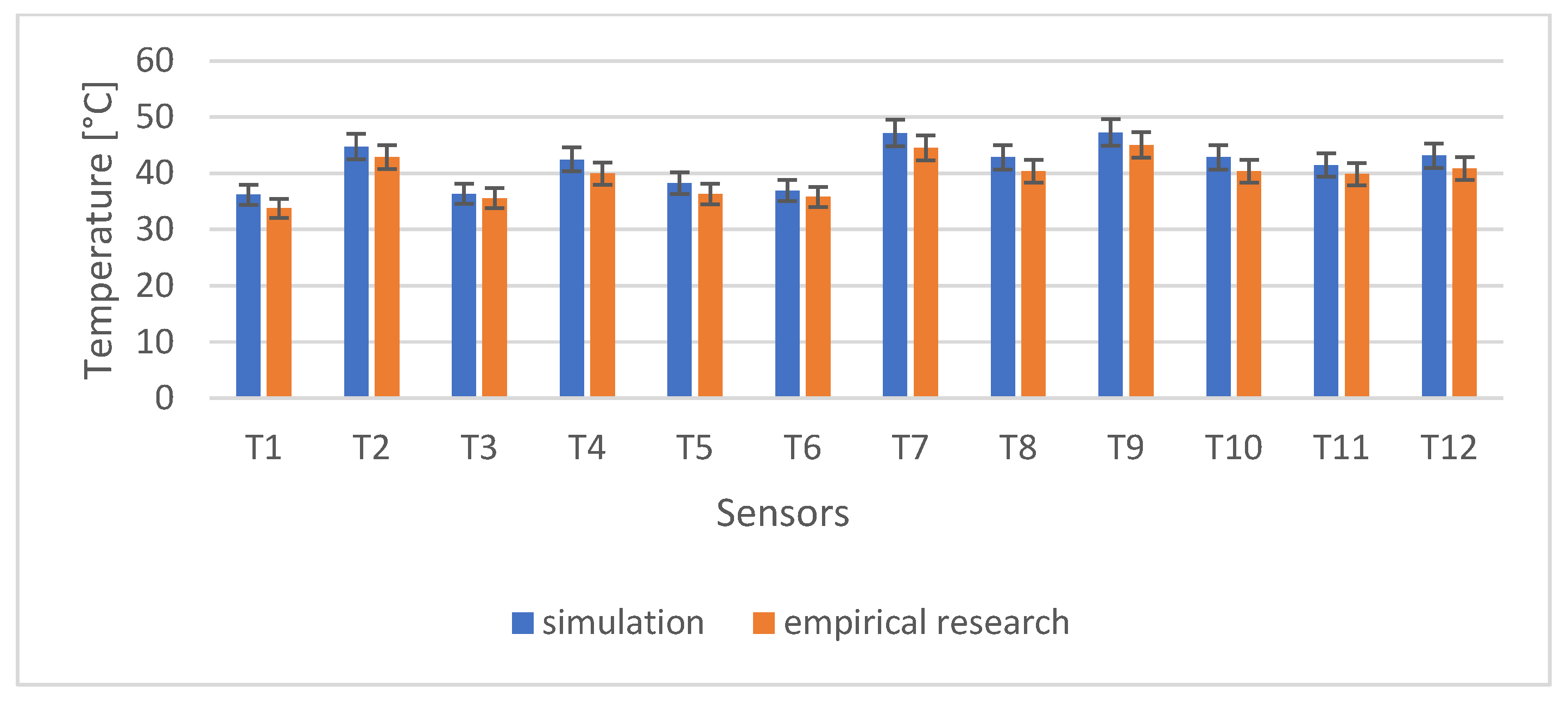
| Measurement Point | T1 | T2 | T3 | T4 | T5 | T6 | T7 | T8 | T9 | T10 | T11 | T12 |
|---|---|---|---|---|---|---|---|---|---|---|---|---|
| Average temperature (°C), simulation | 36.2 | 44.8 | 36.4 | 42.5 | 38.3 | 37.0 | 47.2 | 42.9 | 47.3 | 42.9 | 41.5 | 43.2 |
| Average temperature (°C), experiment | 33.8 | 42.9 | 35.6 | 40.0 | 36.3 | 35.8 | 44.5 | 40.4 | 45.0 | 40.3 | 39.9 | 40.9 |
| Relative difference % | 6.8 | 4.3 | 2.1 | 6.0 | 5.2 | 3.2 | 5.7 | 6.0 | 4.8 | 6.0 | 3.9 | 5.5 |
Disclaimer/Publisher’s Note: The statements, opinions and data contained in all publications are solely those of the individual author(s) and contributor(s) and not of MDPI and/or the editor(s). MDPI and/or the editor(s) disclaim responsibility for any injury to people or property resulting from any ideas, methods, instructions or products referred to in the content. |
© 2024 by the authors. Licensee MDPI, Basel, Switzerland. This article is an open access article distributed under the terms and conditions of the Creative Commons Attribution (CC BY) license (https://creativecommons.org/licenses/by/4.0/).
Share and Cite
Cebulski, D.; Cyklis, P. Application of CFD Simulation to the Design of an Innovative Drying Chamber. Energies 2024, 17, 3338. https://doi.org/10.3390/en17133338
Cebulski D, Cyklis P. Application of CFD Simulation to the Design of an Innovative Drying Chamber. Energies. 2024; 17(13):3338. https://doi.org/10.3390/en17133338
Chicago/Turabian StyleCebulski, Damian, and Piotr Cyklis. 2024. "Application of CFD Simulation to the Design of an Innovative Drying Chamber" Energies 17, no. 13: 3338. https://doi.org/10.3390/en17133338
APA StyleCebulski, D., & Cyklis, P. (2024). Application of CFD Simulation to the Design of an Innovative Drying Chamber. Energies, 17(13), 3338. https://doi.org/10.3390/en17133338