Optimization of the Performance of PCM Thermal Storage Systems

Abstract

In this article, we present some optimised geometries for a thermal storage system previously proposed exploiting Phase-changing materials (PCMs). The optimization has been carried out by using a genetic algorithm. We demonstrate that a simple single-parental, mutation-based, single-objective genetic algorithm can be conveniently employed to optimize the geometry of the proposed PCM thermal energy storage system. Optimization I was the one with the least restrictive conditions and, therefore, with the greatest possibility of variation in the channel geometry. While the one with the worst results is Optimization II because of the most restrictive conditions, primarily constant solid/liquid volume. A metal frame increases the surface area by 6.

1. Introduction

Phase-change materials (PCM) have been demonstrated to be particularly useful in thermal energy storage systems [1]. The main worth they offer comes from their capability of accumulating a large amount of heat by slightly varying their temperature. In general, this allows PCM to exchange constant and high heat fluxes with constant temperature systems during the charge and discharge of thermal energy. On the other side, PCM can contribute to keeping constant and lowering the temperature of a system, improving its performance. This is the case of PCM, which directly removes and stores the heat generated by the solar radiation in a photo-voltaic layer, whose conversion efficiency decreases with the temperature. In the last decade, thermal energy storage systems have been utilized to accumulate the heat provided by solar panels and other sources of renewable energy. In the system exploiting PCM, the body providing the thermal energy usually transfers it to the accumulator directly or through a vector fluid. The heat transfer efficiency plays a key role in thermal storage since it influences the exchanged thermal power and charge and discharge time of the accumulator [2,3,4,5,6,7,8,9,10,11,12,13,14,15,16]. Particularly, Cabeza et al. [4] show three methods to enhance the heat transfer in a cold storage working with water/ice as PCM: addition of stainless-steel pieces, copper pieces (both have been proposed before) and a new PCM–graphite composite material are compared. The PCM–graphite composite material showed an increase in heat flux bigger than with any of the other techniques. Stritih [11] and Erek [14] have studied the heat-transfer characteristics of a latent-heat storage unit with a finned surface in terms of the solidification and melting processes comparing different heat storage geometries. Genetic algorithms were first proposed by Bagley [17] in 1967 as an optimization method inspired by the evolution of biological species. They were then developed in the course of the 1970s as adaptive systems [18]. The optimization method was further improved in the 1980s [19]. In the mid-1990s, genetic algorithms began to be used for the solution of optimization problems in the heat transfer and fluid flow sector [20,21]. In the course of time, they have been applied to the design of heat sinks [22] and their components, of air conditioning systems [23,24] and of thermal plants of power generation [25,26]. Various kinds of genetic algorithms have been proposed and applied to thermal sciences [27], having an increasingly complex structure. The most common of them consider populations of parameter combinations reproduced from one or two parents through random mutations, crossing-overs, or both operations of parental parameters. Moreover, they have been applied to the maximization of a single function or several (multi-objective). However, as we demonstrate in the following, a simple single-parental, mutation-based, single-objective genetic algorithm can be conveniently employed to optimize the geometry of the proposed PCM thermal energy storage system. In a previous work [28], we proposed a new thermal storage system composed of several rectangular section channels surrounded by a PCM and crossed by a vector fluid. We also presented a parametric analysis showing that the channel geometry noticeably influences the heat transfer efficiency and the accumulation time. Actually, the channel geometry determines the heat transfer area and influences the convection coefficient in a complex way. In this article, we present some optimized geometries for the thermal storage system previously proposed. The optimization has been carried out by using a genetic algorithm. The reproduction parameters considered in the optimization are L_y1, L_y2, L_z, the value of the ordinate z, relative to the n points used to derive, by interpolation, the polynomial of degree n of the channel wall and some parameters describing the profiles of the channels.

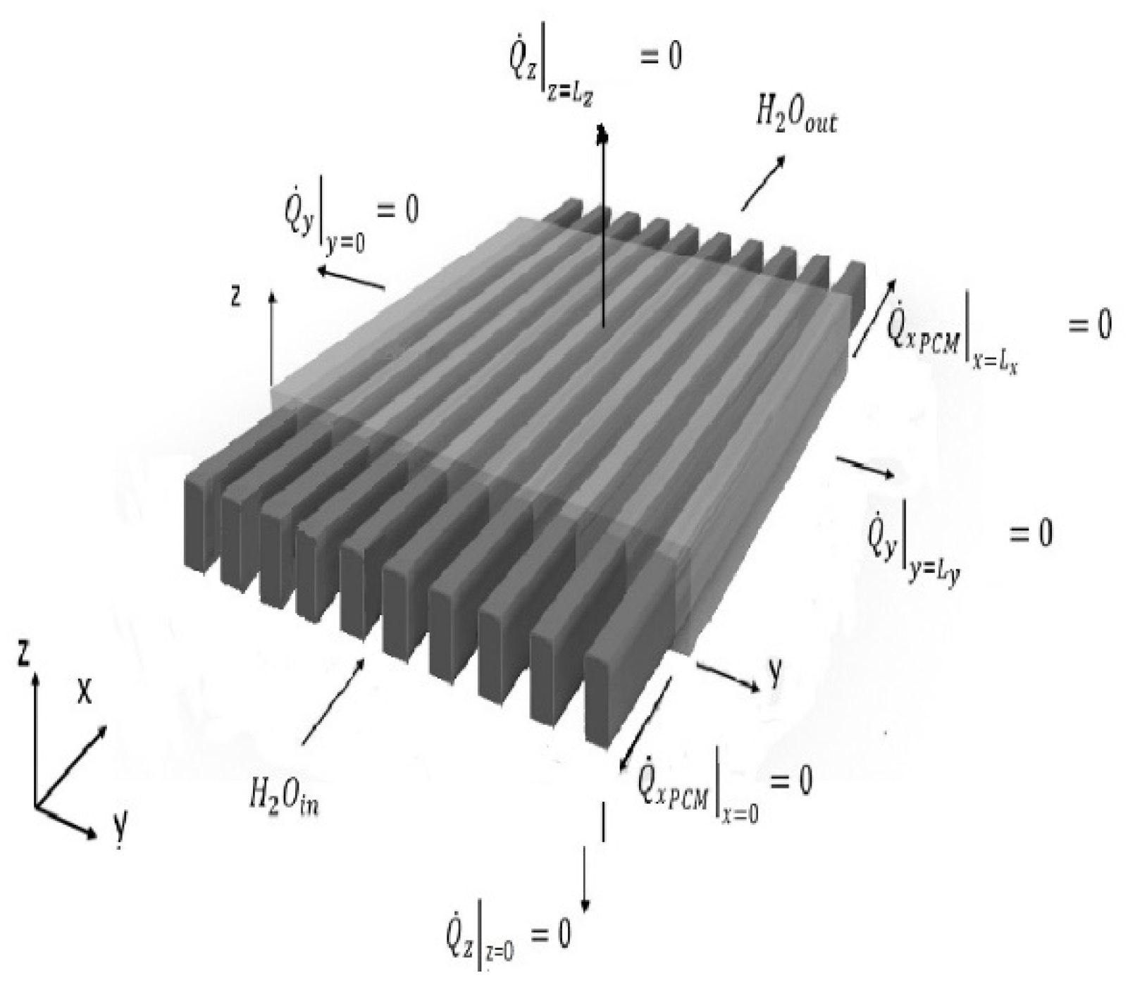
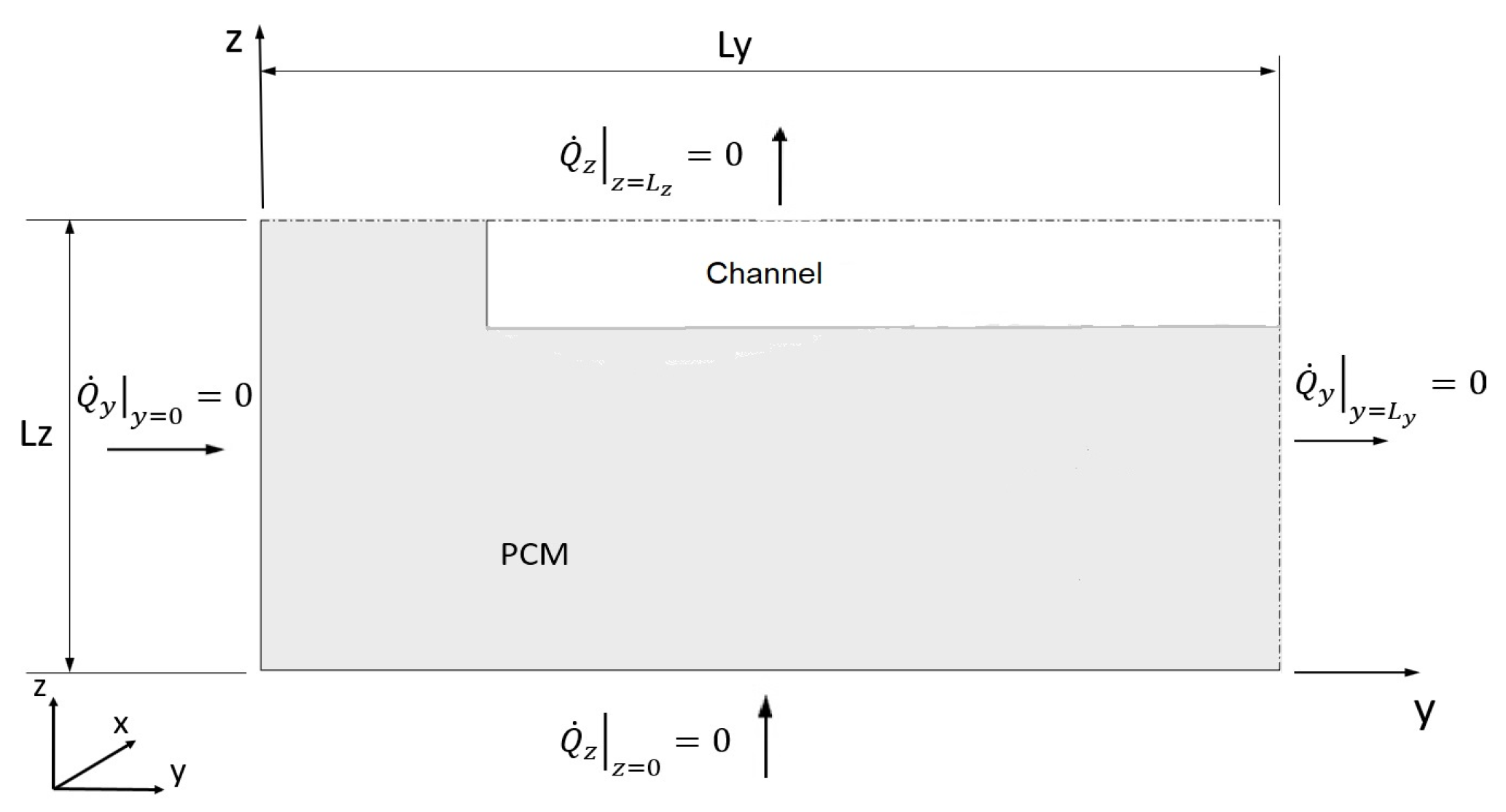
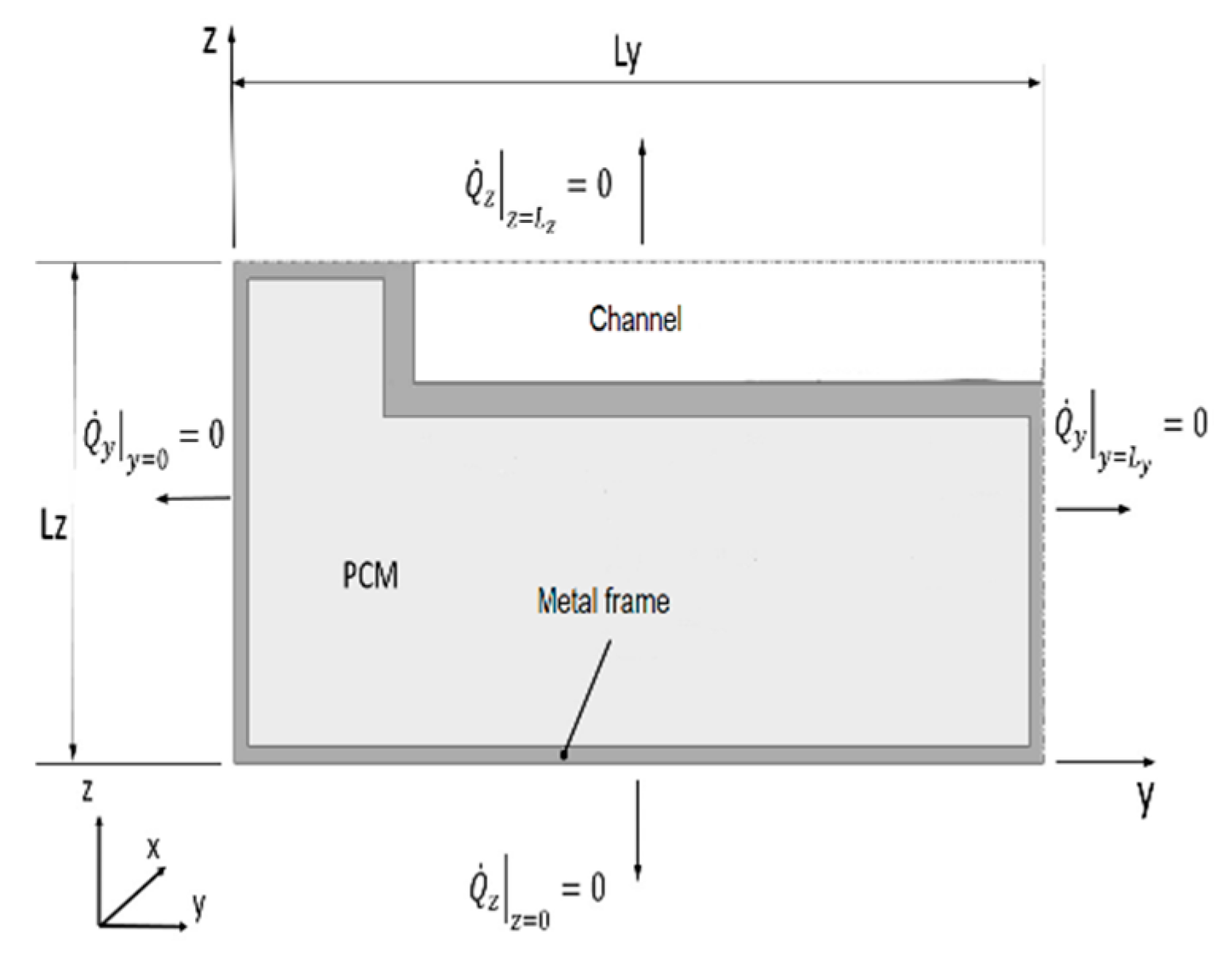
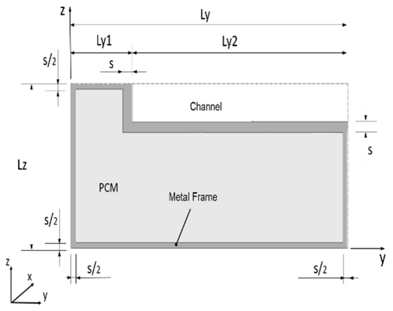
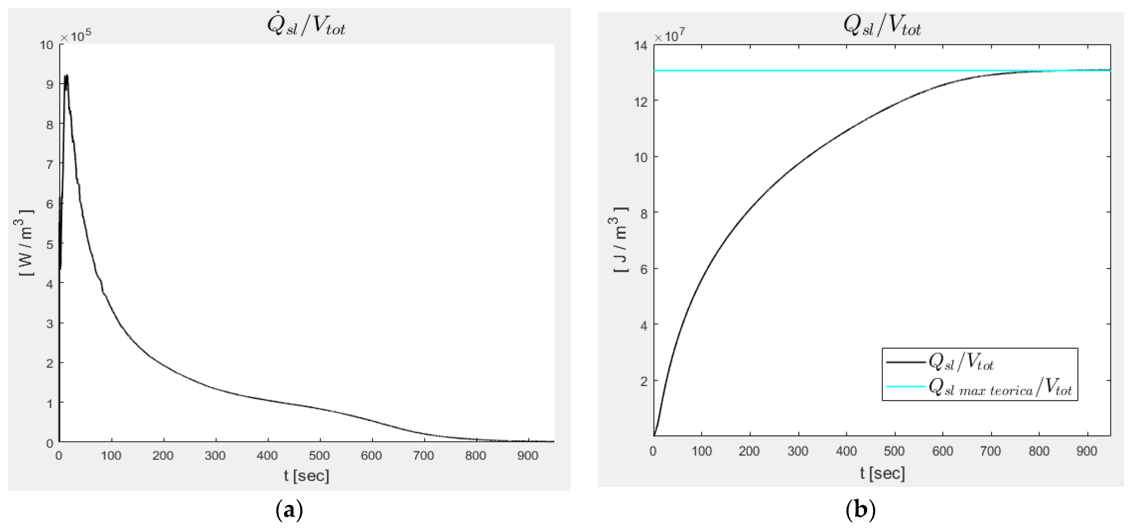
2. PCM Heat Storage

The heat storage system that has been optimized is shown in Figure 1 and Figure 2. It is composed of 10 channels having four thin metal walls surrounded by a PCM. In the case analyzed in the previous work [28], all walls were flat, thus resulting in rectangular channels. In the optimized cases presented in this work, the profiles of two opposite walls are described by polynomial functions whose parameters must be optimized. In Figure 1, the channels are dark-grey-colored and the PCMs are grey-transparent-colored. Inside the channels, a thermal vector fluid flows. The parts of the channels not surrounded by the PCM are thermally insulated. They are long enough to ensure that the velocity profile of the fluid entering the PCM section is completely developed and output phenomena are negligible. Boundary conditions and governing equations are largely described in [28].

In Figure 3, the cross-section of the studied domain (CHANNEL A) is shown. It consists of a channel surrounded by PCM and delimited by symmetry axes.

The profiles of the upper and the lower walls are described by polynomial functions. In Figure 2, these functions are constant. If the profiles analyzed for the upper and the lower walls are symmetrical in the y direction the studied domain reduces to that represented in Figure 4.

As in the previous work, the governing equations have been integrated by using a composite finite volume and finite difference method. In particular, the studied spatial domain (Figure 3 or Figure 4) has been divided into finite dimensions prismatic volumes, disposed in layers along the x axis. The integration of the differential equations in the time dimension has been carried out using the finite difference method. Starting from an initial distribution of velocity, temperature and PCM liquid concentration for each finite volume of the spatial domain, changes in the latent and sensible thermal energy have been calculated for each prism and then the distribution of velocity, temperature and PCM liquid concentration for the new time step have been obtained. The procedure has been iterated until a final instant has been reached.

CHANNEL B

The geometry of the channel referred to as Channel A, with the addition of the aluminum frame of thickness ${\mathrm{s}}_{\mathrm{m}\mathrm{e}}=5·{10}^{-4} \mathrm{m}$, is shown in Figure 5 and Figure 6.

This channel configuration is derived from the previous CHANNEL A.

Thus, many of the same considerations made for CHANNEL A are used, with the only difference being that a thin metal frame is adopted (aluminum could be used for both technical and technological reasons), which encloses the solid/liquid material (PCM). During the first numerical simulations on case A, it was found that one of the problems in heat propagation is that liquid paraffin has a lower thermal conductivity than solid paraffin.

$${\mathrm{k}}_{\mathrm{s}}=0.4\frac{\mathrm{W}}{\mathrm{m}°\mathrm{C}},{\mathrm{k}}_{\mathrm{l}}=0.2\frac{\mathrm{W}}{\mathrm{m}°\mathrm{C}}$$

As a result, it occurs that, as soon as the paraffin, near the channel crossed by the hot fluid, melts, the thermal conductivity is lowered, resulting in a slowdown in heat conduction within the domain. If the channel with the metal wall were to be considered, the wall thermal resistance would be negligible compared to the others. But, as can be seen from Figure 5 in this case, a frame part has been added to enclose the solid/liquid material of each quarter module. This type of metal frame could have a positive effect on heat transfer within the studied domain. Since metal has a high thermal conductivity, heat passes quickly from the fluid to the entire metal frame, increasing heat transfer surface area. This could lead to a shorter charging time of the heat accumulator. This hypothesis will then be verified with appropriate numerical simulations described in the following chapters. The boundary conditions are the same as those described for CHANNEL A.

3. Optimization

The geometry of the studied domain has been optimized by using a single-parental, mutation-based, single-objective genetic algorithm. The populations of parameter combinations were composed of 10 samples, out of which the best-performing 2 were selected and reproduced with random mutations. The algorithm was stopped after 50 generations with no improvement in the heat storage performance. The reproduction parameters considered in the optimization are L_y1, L_y2, L_z, the value of the ordinate z, relative to the n points used to derive, by interpolation, the polynomial of degree n of the channel wall and some parameters describing the profiles of the channels. Different kinds of optimization have been carried out considering different kinds of domains:

I: Optimization at constant charge energy;

II: Optimization at constant charge energy and constant paraffin volume

Optimization I;

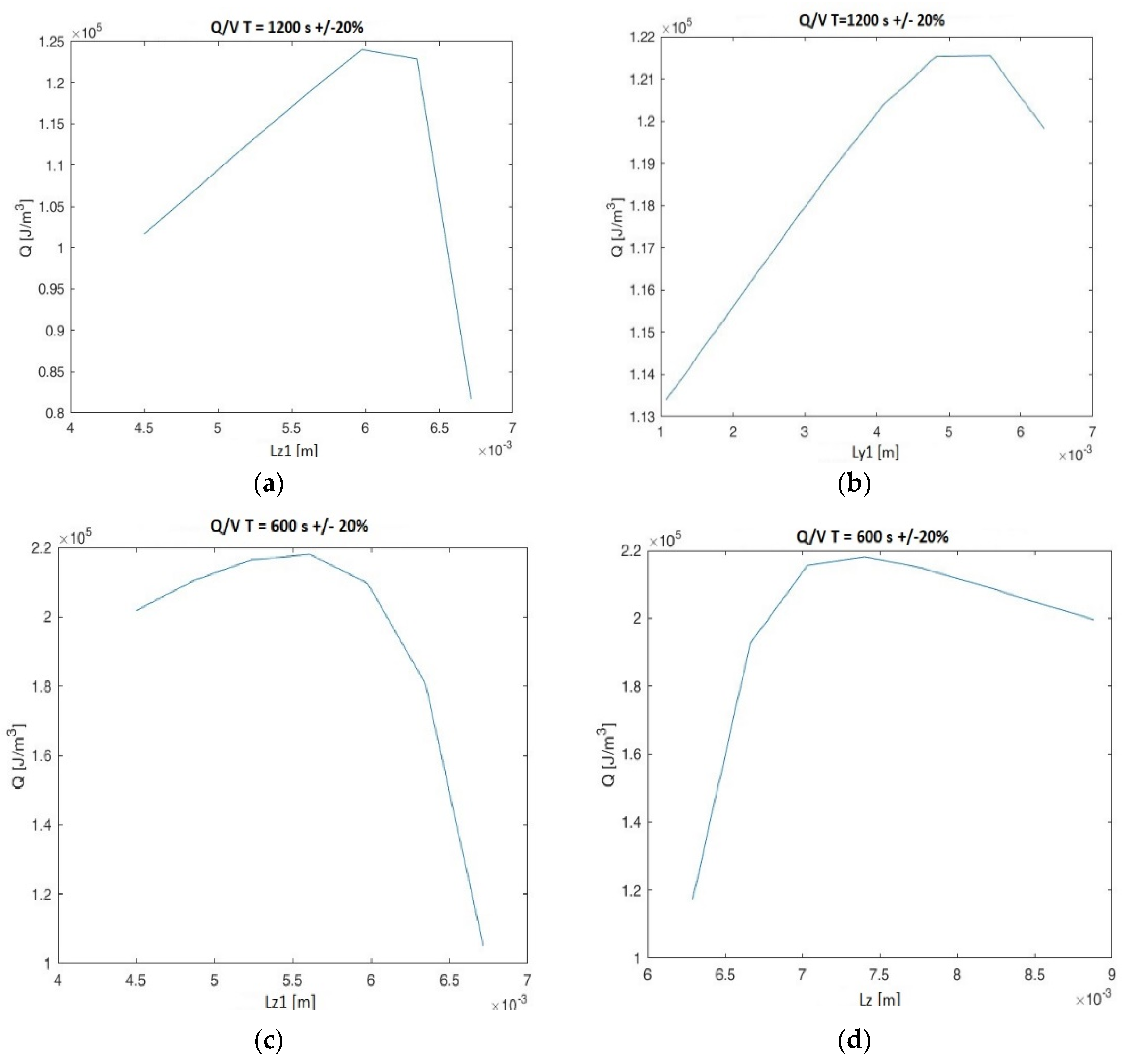
• Optimization I-2: Type I optimization of a type A channel, with polynomial degree of the channel wall n = 2;
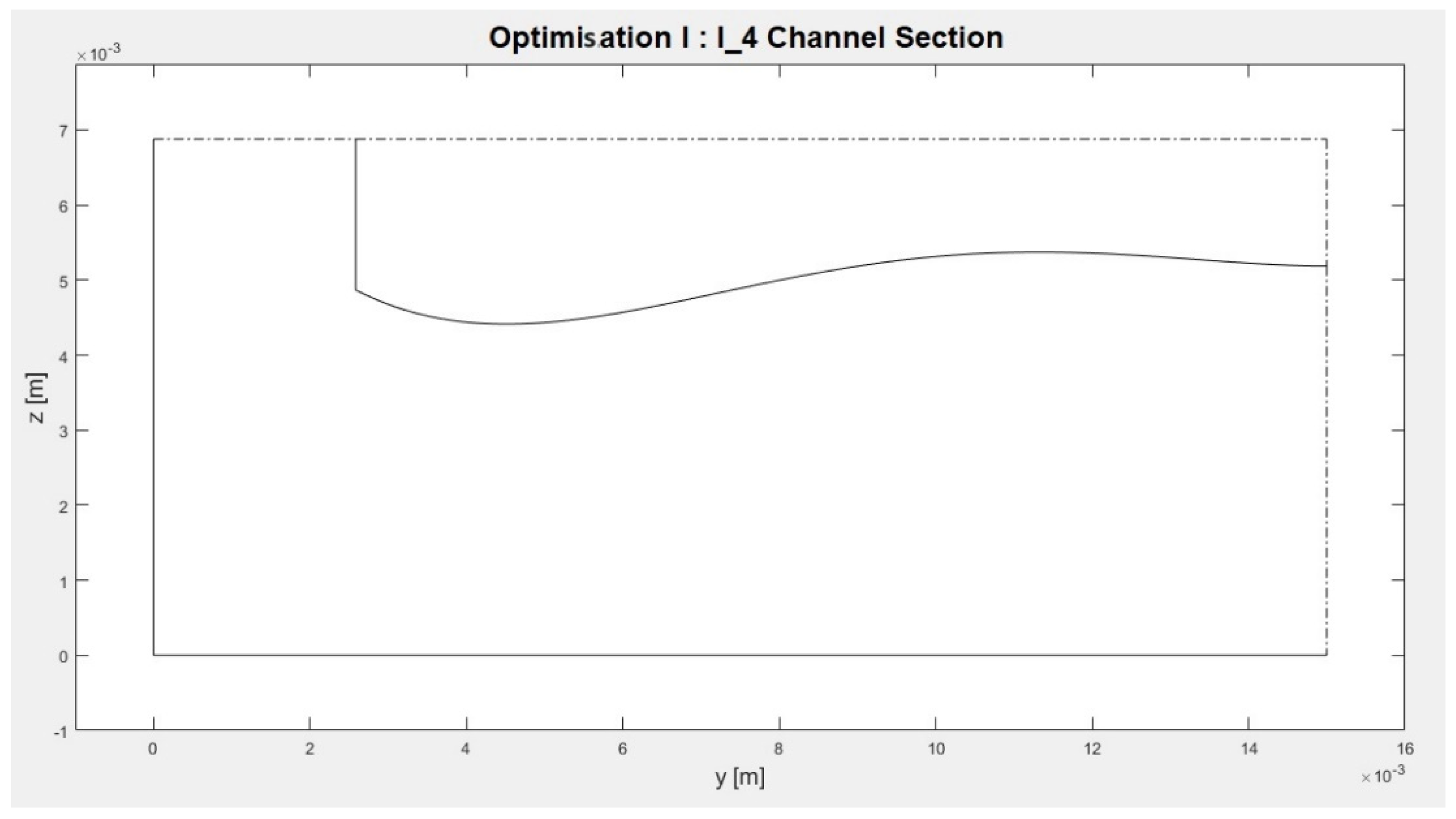
• Optimization I-4: Type I optimization of a type A channel, with polynomial degree of the channel wall n = 4.

Afterwards, the performance of B-type channels whose basic geometry is the result of optimization I-2 was also evaluated.

Optimization I-2: channel A

The geometry of the channel obtained through optimization I-2 is shown in Figure 7.

And it is described by the following parameters (

Table 1. Channel A: section parameters (I-2).

${\mathrm{z}}_{\mathrm{p}2}\left[\mathrm{m}\right]$	${\mathrm{z}}_{\mathrm{p}1}\left[\mathrm{m}\right]$	${\mathrm{L}}_{\mathrm{z}}\left[\mathrm{m}\right]$	${\mathrm{L}}_{\mathrm{y}2}\left[\mathrm{m}\right]$	${\mathrm{L}}_{\mathrm{y}1}\left[\mathrm{m}\right]$
$0.004558$	$0.003845$	$0.006118$	$0.011731$	$0.003268$
${\mathrm{V}}_{\mathrm{t}\mathrm{o}\mathrm{t}}\left[{\mathrm{m}}^3\right]$	${\mathrm{V}}_{\mathrm{s}\mathrm{l}}\left[{\mathrm{m}}^3\right]$		${\mathrm{V}}_{\mathrm{f}}\left[{\mathrm{m}}^3\right]$
$1.8356·{10}^{-5}$	$1.4136·{10}^{-5}$		$4.2193·{10}^{-6}$
${\mathrm{A}}_{\mathrm{t}\mathrm{o}\mathrm{t}}\left[{\mathrm{m}}^2\right]$	${\mathrm{A}}_{\mathrm{s}\mathrm{l}}\left[{\mathrm{m}}^2\right]$		${\mathrm{A}}_{\mathrm{f}}\left[{\mathrm{m}}^2\right]$
$9.1781·{10}^{-5}$	$7.0684·{10}^{-5}$		$2.1097·{10}^{-5}$
$\frac{{\mathrm{V}}_{\mathrm{s}\mathrm{l}}}{{\mathrm{V}}_{\mathrm{t}\mathrm{o}\mathrm{t}}}$			Vf/Vtot
$0.7701$			$0.2299$
${\dot{\mathrm{V}}}_{\mathrm{f}}\left[{\mathrm{m}}^3/\mathrm{s}\right]$	$\overline{\mathrm{u}}\left[\mathrm{m}/\mathrm{s}\right]$		${\mathrm{u}}_{\mathrm{m}\mathrm{a}\mathrm{x}}\left[\mathrm{m}/\mathrm{s}\right]$
$1.8176·{10}^{-7}$	$0.0086$		$0.0163$

).

The velocity field is represented by Figure 8.

The time course of the temperature field is qualitatively comparable to that of the reference channel. The time trends of the energy density and the power density are depicted in Figure 9a,b.

Below are the values of the performance parameters.

${\mathrm{t}}_{{\mathrm{Q}}_{\mathrm{s}\mathrm{l}\mathrm{m}\mathrm{a}\mathrm{x}}99\%}\left[\mathrm{s}\right]$	${\mathrm{t}}_{{\mathrm{Q}}_{\mathrm{s}\mathrm{l}\mathrm{m}\mathrm{a}\mathrm{x}}90\%}\left[\mathrm{s}\right]$	${\mathrm{t}}_{{\mathrm{Q}}_{\mathrm{s}\mathrm{l}\mathrm{r}\mathrm{e}\mathrm{f}}}\left[\mathrm{s}\right]$
$567.52$	$362.6$	$288.7$

$$\frac{{\mathrm{Q}}_{\mathrm{s}\mathrm{l}\mathrm{r}\mathrm{e}\mathrm{f}}}{{\mathrm{V}}_{\mathrm{t}\mathrm{o}\mathrm{t}\mathrm{r}\mathrm{e}\mathrm{f}}}=1.0933·{10}^8 \mathrm{J}/{\mathrm{m}}^3$$

$$\frac{{\mathrm{Q}}_{\mathrm{s}\mathrm{l}\mathrm{m}\mathrm{a}\mathrm{x}}}{{\mathrm{V}}_{\mathrm{t}\mathrm{o}\mathrm{t}}}=1.3494·{10}^8 \mathrm{J}/{\mathrm{m}}^3$$

$$\frac{{\mathrm{Q}}_{\mathrm{s}\mathrm{l}\mathrm{r}\mathrm{e}\mathrm{f}}}{{\mathrm{V}}_{\mathrm{t}\mathrm{o}\mathrm{t}\mathrm{r}\mathrm{e}\mathrm{f}}}·\frac{{\mathrm{V}}_{\mathrm{t}\mathrm{o}\mathrm{t}}}{{\mathrm{Q}}_{\mathrm{s}\mathrm{l}\mathrm{m}\mathrm{a}\mathrm{x}}}=0.8102$$

$$\frac{{\left.{\overline{\dot{\mathrm{Q}}}}_{\mathrm{s}\mathrm{l}}\right|}_{\mathrm{t}={\mathrm{t}}_{{\mathrm{Q}}_{\mathrm{s}\mathrm{l}\mathrm{r}\mathrm{e}\mathrm{f}}}}}{{\mathrm{V}}_{\mathrm{t}\mathrm{o}\mathrm{t}}}=3.7871·{10}^5 \mathrm{W}/{\mathrm{m}}^3$$

$$\frac{{\left.{\overline{\dot{\mathrm{Q}}}}_{\mathrm{s}\mathrm{l}}\right|}_{\mathrm{t}={\mathrm{t}}_{{\mathrm{Q}}_{\mathrm{s}\mathrm{l}\mathrm{m}\mathrm{a}\mathrm{x}}90\%}}}{{\mathrm{V}}_{\mathrm{t}\mathrm{o}\mathrm{t}}}=3.3493·{10}^5 \mathrm{W}/{\mathrm{m}}^3$$

$$\frac{{\left.{\overline{\dot{\mathrm{Q}}}}_{\mathrm{s}\mathrm{l}}\right|}_{\mathrm{t}={\mathrm{t}}_{{\mathrm{Q}}_{\mathrm{s}\mathrm{l}\mathrm{m}\mathrm{a}\mathrm{x}}99\%}}}{{\mathrm{V}}_{\mathrm{t}\mathrm{o}\mathrm{t}}}=2.3522·{10}^5 \mathrm{W}/{\mathrm{m}}^3$$

Optimization I_4: channel A

The geometry of the channel obtained through optimization I-4 is shown in Figure 10.

And it is described by the following parameters (

Table 2. Channel A: section parameters (I-4).

${\mathrm{z}}_{\mathrm{p}4}\left[\mathrm{m}\right]$	${\mathrm{z}}_{\mathrm{p}3}\left[\mathrm{m}\right]$	${\mathrm{z}}_{\mathrm{p}2}\left[\mathrm{m}\right]$	${\mathrm{z}}_{\mathrm{p}1}\left[\mathrm{m}\right]$	${\mathrm{L}}_{\mathrm{z}}\left[\mathrm{m}\right]$	${\mathrm{L}}_{\mathrm{y}2}\left[\mathrm{m}\right]$
$0.005186$	$0.005365$	$0.004717$	$0.004867$	$0.006878$	$0.012415$
${\mathrm{V}}_{\mathrm{t}\mathrm{o}\mathrm{t}}\left[{\mathrm{m}}^3\right]$	${\mathrm{V}}_{\mathrm{s}\mathrm{l}}\left[{\mathrm{m}}^3\right]$			${\mathrm{V}}_{\mathrm{f}}\left[{\mathrm{m}}^3\right]$
$2.0635·{10}^{-5}$	$1.593·{10}^{-5}$			$4.7037·{10}^{-6}$
${\mathrm{A}}_{\mathrm{t}\mathrm{o}\mathrm{t}}\left[{\mathrm{m}}^2\right]$	${\mathrm{A}}_{\mathrm{s}\mathrm{l}}\left[{\mathrm{m}}^2\right]$			${\mathrm{A}}_{\mathrm{f}}\left[{\mathrm{m}}^2\right]$
$1.0317·{10}^{-4}$	$7.9654·{10}^{-5}$			$2.3519·{10}^{-5}$
$\frac{{\mathrm{V}}_{\mathrm{s}\mathrm{l}}}{{\mathrm{V}}_{\mathrm{t}\mathrm{o}\mathrm{t}}}$			$\frac{{\mathrm{V}}_{\mathrm{f}}}{{\mathrm{V}}_{\mathrm{t}\mathrm{o}\mathrm{t}}}$
$0.772$			$0.228$

).

The velocity field is depicted in Figure 11.

${\dot{\mathrm{V}}}_{\mathrm{f}}\left[{\mathrm{m}}^3/\mathrm{s}\right]$	$\overline{\mathrm{u}}\left[\mathrm{m}/\mathrm{s}\right]$	${\mathrm{u}}_{\mathrm{m}\mathrm{a}\mathrm{x}}\left[\mathrm{m}/\mathrm{s}\right]$
$2.2979·{10}^{-7}$	$0.0098$	$0.0204$

The time course of the temperature field, on a qualitative level, is similar to that of the reference channel. The time trends of the energy and thermal power density are similar, qualitatively and quantitatively, to those obtained from the II-2 optimization. Below are the values of the performance parameters.

${\mathrm{t}}_{{\mathrm{Q}}_{\mathrm{s}\mathrm{l}\mathrm{m}\mathrm{a}\mathrm{x}}99\%}\left[\mathrm{s}\right]$	${\mathrm{t}}_{{\mathrm{Q}}_{\mathrm{s}\mathrm{l}\mathrm{m}\mathrm{a}\mathrm{x}}90\%}\left[\mathrm{s}\right]$	${\mathrm{t}}_{{\mathrm{Q}}_{\mathrm{s}\mathrm{l}\mathrm{r}\mathrm{e}\mathrm{f}}}\left[\mathrm{s}\right]$
$569.02$	$396.5$	$306.84$

$$\frac{{\mathrm{Q}}_{\mathrm{s}\mathrm{l}\mathrm{m}\mathrm{a}\mathrm{x}}}{{\mathrm{V}}_{\mathrm{t}\mathrm{o}\mathrm{t}}}=1.3527·{10}^8 \mathrm{J}/{\mathrm{m}}^3$$

$$\frac{{\mathrm{Q}}_{\mathrm{s}\mathrm{l}\mathrm{r}\mathrm{e}\mathrm{f}}}{{\mathrm{V}}_{\mathrm{t}\mathrm{o}\mathrm{t}\mathrm{r}\mathrm{e}\mathrm{f}}}·\frac{{\mathrm{V}}_{\mathrm{t}\mathrm{o}\mathrm{t}}}{{\mathrm{Q}}_{\mathrm{s}\mathrm{l}\mathrm{m}\mathrm{a}\mathrm{x}}}=0.8082$$

$$\frac{{\left.{\overline{\dot{\mathrm{Q}}}}_{\mathrm{s}\mathrm{l}}\right|}_{\mathrm{t}={\mathrm{t}}_{{\mathrm{Q}}_{\mathrm{s}\mathrm{l}\mathrm{r}\mathrm{e}\mathrm{f}}}}}{{\mathrm{V}}_{\mathrm{t}\mathrm{o}\mathrm{t}}}=3.5632·{10}^5 \mathrm{W}/{\mathrm{m}}^3$$

$$\frac{{\left.{\overline{\dot{\mathrm{Q}}}}_{\mathrm{s}\mathrm{l}}\right|}_{\mathrm{t}={\mathrm{t}}_{{\mathrm{Q}}_{\mathrm{s}\mathrm{l}\mathrm{m}\mathrm{a}\mathrm{x}}90\%}}}{{\mathrm{V}}_{\mathrm{t}\mathrm{o}\mathrm{t}}}=3.0704·{10}^5 \mathrm{W}/{\mathrm{m}}^3$$

$$\frac{{\left.{\overline{\dot{\mathrm{Q}}}}_{\mathrm{s}\mathrm{l}}\right|}_{\mathrm{t}{\mathrm{t}}_{{\mathrm{Q}}_{\mathrm{s}\mathrm{l}\mathrm{m}\mathrm{a}\mathrm{x}}99\%}}}{{\mathrm{V}}_{\mathrm{t}\mathrm{o}\mathrm{t}}}=2.3535·{10}^5 \mathrm{W}/{\mathrm{m}}^3$$

Optimization I_2 case channel B s_me = 0.0005 m

The main purpose of this simulation is to compare the performance of B channels with different metal frame thicknesses. Parameters are described in following

Table 3. Channel B: section (I-2) s_me = 0.0005.

${\mathrm{V}}_{\mathrm{s}\mathrm{l}}\left[{\mathrm{m}}^3\right]$	${\mathrm{V}}_{\mathrm{m}\mathrm{e}}\left[{\mathrm{m}}^3\right]$
$1.1321·{10}^{-5}$	$2.8094·{10}^{-6}$
${\mathrm{A}}_{\mathrm{s}\mathrm{l}}\left[{\mathrm{m}}^2\right]$	${\mathrm{A}}_{\mathrm{m}\mathrm{e}}\left[{\mathrm{m}}^2\right]$
$5.6605·{10}^{-5}$	$1.4047·{10}^{-5}$
$\frac{{\mathrm{V}}_{\mathrm{s}\mathrm{l}}}{{\mathrm{V}}_{\mathrm{t}\mathrm{o}\mathrm{t}}}$	$\frac{{\mathrm{V}}_{\mathrm{m}\mathrm{e}}}{{\mathrm{V}}_{\mathrm{t}\mathrm{o}\mathrm{t}}}$
$0.6158$	$0.1528$

.

Figure 12a,b show the time course of the accumulated energy and power density.

Below are the values of the most interesting performance parameters.

${\mathrm{t}}_{{\mathrm{Q}}_{\mathrm{s}\mathrm{l}+\mathrm{m}\mathrm{e}\mathrm{m}\mathrm{a}\mathrm{x}}99\%}\left[\mathrm{s}\right]$	${\mathrm{t}}_{{\mathrm{Q}}_{\mathrm{s}\mathrm{l}+\mathrm{m}\mathrm{e}\mathrm{m}\mathrm{a}\mathrm{x}}90\%}\left[\mathrm{s}\right]$	${\mathrm{t}}_{{\mathrm{Q}}_{\mathrm{s}\mathrm{l}+\mathrm{m}\mathrm{e}\mathrm{r}\mathrm{e}\mathrm{f}}}\left[\mathrm{s}\right]$
$194.02$	$140.24$	$122.66$

${\mathrm{t}}_{{\mathrm{Q}}_{\mathrm{s}\mathrm{l}+\mathrm{m}\mathrm{e}\mathrm{r}\mathrm{e}\mathrm{f}}}$: time in which an energy density equal to the reference value is accumulated (1.0933 * 10 ⁸ J/m³), obtained from the simulation of the reference A channel.

$$\frac{{\mathrm{Q}}_{\mathrm{s}\mathrm{l}+\mathrm{m}\mathrm{e}\mathrm{m}\mathrm{a}\mathrm{x}}}{{\mathrm{V}}_{\mathrm{t}\mathrm{o}\mathrm{t}}}=1.2969·{10}^8\mathrm{J}/{\mathrm{m}}^3$$

$\frac{{\left.{\overline{\dot{\mathrm{Q}}}}_{\mathrm{s}\mathrm{l}+\mathrm{m}\mathrm{e}}\right|}_{\mathrm{t}={\mathrm{t}}_{{\mathrm{Q}}_{\mathrm{s}\mathrm{l}+\mathrm{m}\mathrm{e}\mathrm{r}\mathrm{e}\mathrm{f}}}}}{{\mathrm{V}}_{\mathrm{t}\mathrm{o}\mathrm{t}}}=8.9135·{10}^5\mathrm{W}/{\mathrm{m}}^3$: average accumulated thermal power density at time ${\mathrm{t}}_{{\mathrm{Q}}_{\mathrm{s}\mathrm{l}+\mathrm{m}\mathrm{e}\mathrm{r}\mathrm{e}\mathrm{f}}}$

$$\frac{{\left.{\overline{\dot{\mathrm{Q}}}}_{\mathrm{s}\mathrm{l}+\mathrm{m}\mathrm{e}}\right|}_{\mathrm{t}={\mathrm{t}}_{{\mathrm{Q}}_{\mathrm{s}\mathrm{l}+\mathrm{m}\mathrm{e}\mathrm{m}\mathrm{a}\mathrm{x}}90\%}}}{{\mathrm{V}}_{\mathrm{t}\mathrm{o}\mathrm{t}}}=8.3229·{10}^5 \mathrm{W}/{\mathrm{m}}^3$$

$$\frac{{\left.{\overline{\dot{\mathrm{Q}}}}_{\mathrm{s}\mathrm{l}+\mathrm{m}\mathrm{e}}\right|}_{\mathrm{t}={\mathrm{t}}_{{\mathrm{Q}}_{\mathrm{s}\mathrm{l}+\mathrm{m}\mathrm{e}\mathrm{m}\mathrm{a}\mathrm{x}}99\%}}}{{\mathrm{V}}_{\mathrm{t}\mathrm{o}\mathrm{t}}}=6.6175·{10}^5 \mathrm{W}/{\mathrm{m}}^3$$

Optimization I-2 case channel B s_{me frame} = 0.001

For the geometry of the channel, refer to Optimization I-2, with the addition of the metal frame of thickness s_me = 10⁻³ m. The geometric parameters are listed below (

Table 4. Channel B: section parameters (I-2) s_me = 0.001 m.

${\mathrm{V}}_{\mathrm{s}\mathrm{l}}\left[{\mathrm{m}}^3\right]$	${\mathrm{V}}_{\mathrm{m}\mathrm{e}}\left[{\mathrm{m}}^3\right]$
$8.2464·{10}^{-6}$	$5.5437·{10}^{-6}$
${\mathrm{A}}_{\mathrm{s}\mathrm{l}}\left[{\mathrm{m}}^2\right]$	${\mathrm{A}}_{\mathrm{m}\mathrm{e}}\left[{\mathrm{m}}^2\right]$
$4.1232·{10}^{-5}$	$2.7718·{10}^{-5}$
$\frac{{\mathrm{V}}_{\mathrm{s}\mathrm{l}}}{{\mathrm{V}}_{\mathrm{t}\mathrm{o}\mathrm{t}}}$	$\frac{{\mathrm{V}}_{\mathrm{m}\mathrm{e}}}{{\mathrm{V}}_{\mathrm{t}\mathrm{o}\mathrm{t}}}$
$0.4486$	$0.3016$

).

The speed range is the same as in I-2 optimization. The temperature field is qualitatively similar to that described in simulation I-2 channel B. Figure 13a,b show the time course of the energy density and the stored power density.

Below are the values of the performance parameters.

${\mathrm{t}}_{{\mathrm{Q}}_{\mathrm{s}\mathrm{l}+\mathrm{m}\mathrm{e}\mathrm{m}\mathrm{a}\mathrm{x}}99\%}\left[\mathrm{s}\right]$	${\mathrm{t}}_{{\mathrm{Q}}_{\mathrm{s}\mathrm{l}+\mathrm{m}\mathrm{e}\mathrm{m}\mathrm{a}\mathrm{x}}90\%}\left[\mathrm{s}\right]$	${\mathrm{t}}_{{\mathrm{Q}}_{\mathrm{s}\mathrm{l}+\mathrm{m}\mathrm{e}\mathrm{r}\mathrm{e}\mathrm{f}}}\left[\mathrm{s}\right]$
$175.2$	$119.56$	$119.3$

$$\frac{{\mathrm{Q}}_{\mathrm{s}\mathrm{l}+\mathrm{m}\mathrm{e}\mathrm{m}\mathrm{a}\mathrm{x}}}{{\mathrm{V}}_{\mathrm{t}\mathrm{o}\mathrm{t}}}=1.2159·{10}^8 \mathrm{J}/{\mathrm{m}}^3$$

$$\frac{{\left.{\overline{\dot{\mathrm{Q}}}}_{\mathrm{s}\mathrm{l}+\mathrm{m}\mathrm{e}}\right|}_{\mathrm{t}={\mathrm{t}}_{{\mathrm{Q}}_{\mathrm{s}\mathrm{l}+\mathrm{m}\mathrm{e}\mathrm{r}\mathrm{e}\mathrm{f}}}}}{{\mathrm{V}}_{\mathrm{t}\mathrm{o}\mathrm{t}}}=9.1645·{10}^5 \mathrm{W}/{\mathrm{m}}^3$$

$$\frac{{\left.{\overline{\dot{\mathrm{Q}}}}_{\mathrm{s}\mathrm{l}+\mathrm{m}\mathrm{e}}\right|}_{\mathrm{t}={\mathrm{t}}_{{\mathrm{Q}}_{\mathrm{s}\mathrm{l}+\mathrm{m}\mathrm{e}\mathrm{m}\mathrm{a}\mathrm{x}}90\%}}}{{\mathrm{V}}_{\mathrm{t}\mathrm{o}\mathrm{t}}}=9.1526·{10}^5 \mathrm{W}/{\mathrm{m}}^3$$

$$\frac{{\left.{\overline{\dot{\mathrm{Q}}}}_{\mathrm{s}\mathrm{l}+\mathrm{m}\mathrm{e}}\right|}_{\mathrm{t}={\mathrm{t}}_{{\mathrm{Q}}_{\mathrm{s}\mathrm{l}+\mathrm{m}\mathrm{e}\mathrm{m}\mathrm{a}\mathrm{x}}99\%}}}{{\mathrm{V}}_{\mathrm{t}\mathrm{o}\mathrm{t}}}=6.8705·{10}^5 \mathrm{W}/{\mathrm{m}}^3$$

Compared to the analogous simulation made with a B channel with a metal frame of thickness, this simulation finds:

-

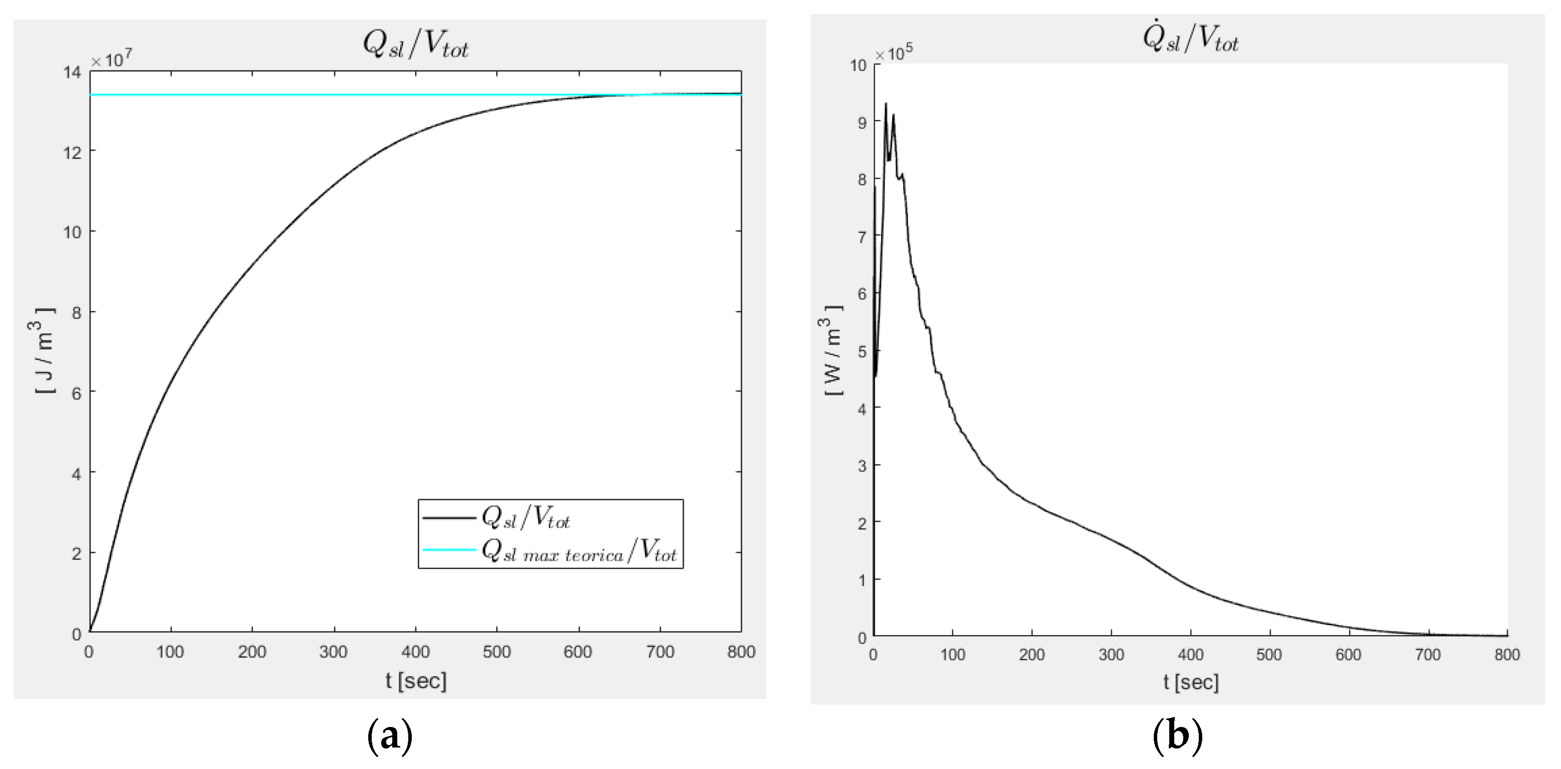
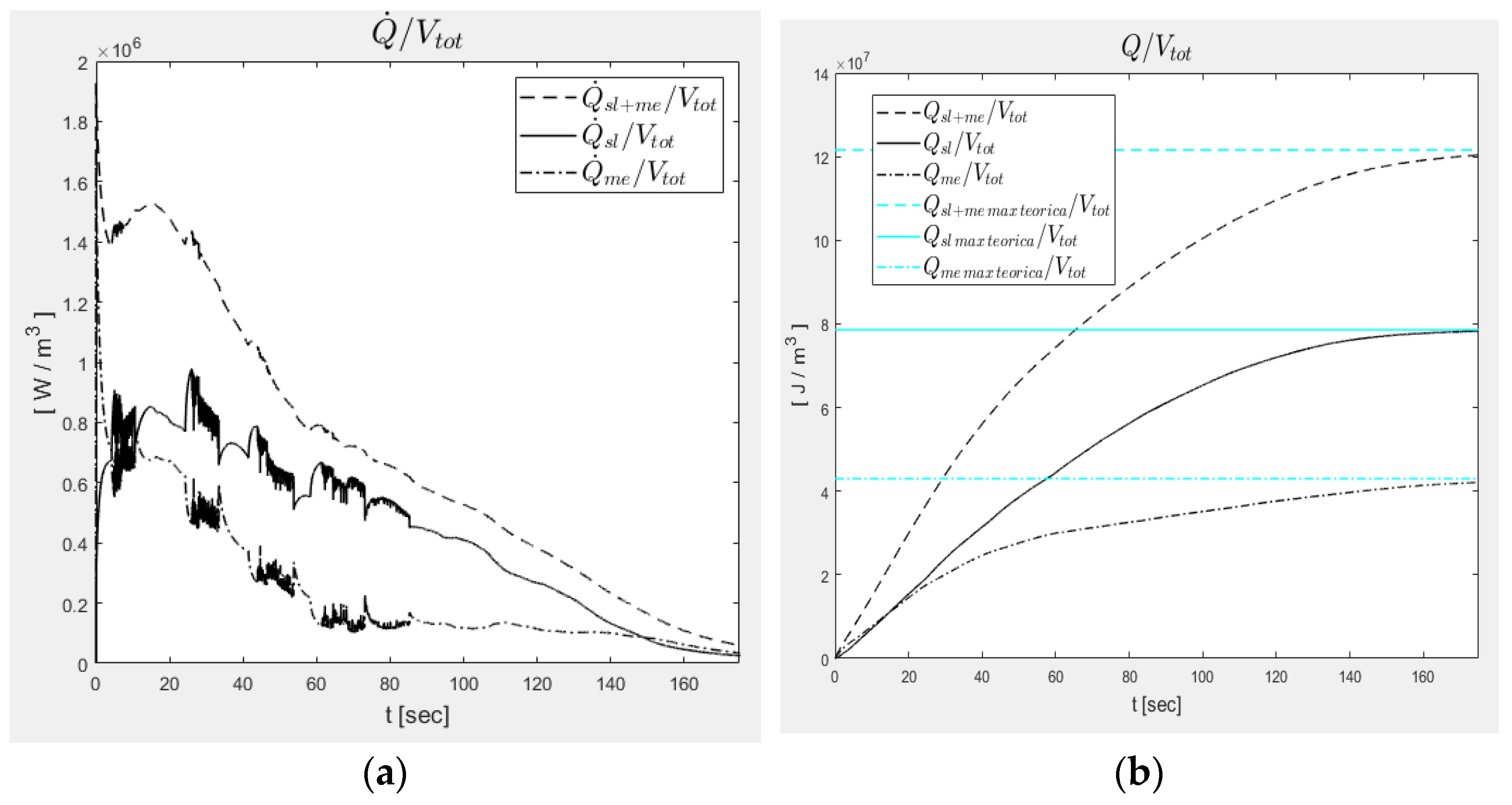
An increase in energy density and thermal power density accumulated by the metal;

-

A decrease in energy density and thermal power density stored by the solid/liquid material;

-

A slight decrease in maximum storable energy density;

-

A comparable heat transfer rate.

Optimization II

In this section, Optimization II is presented. Two Type II optimizations were carried out:

-

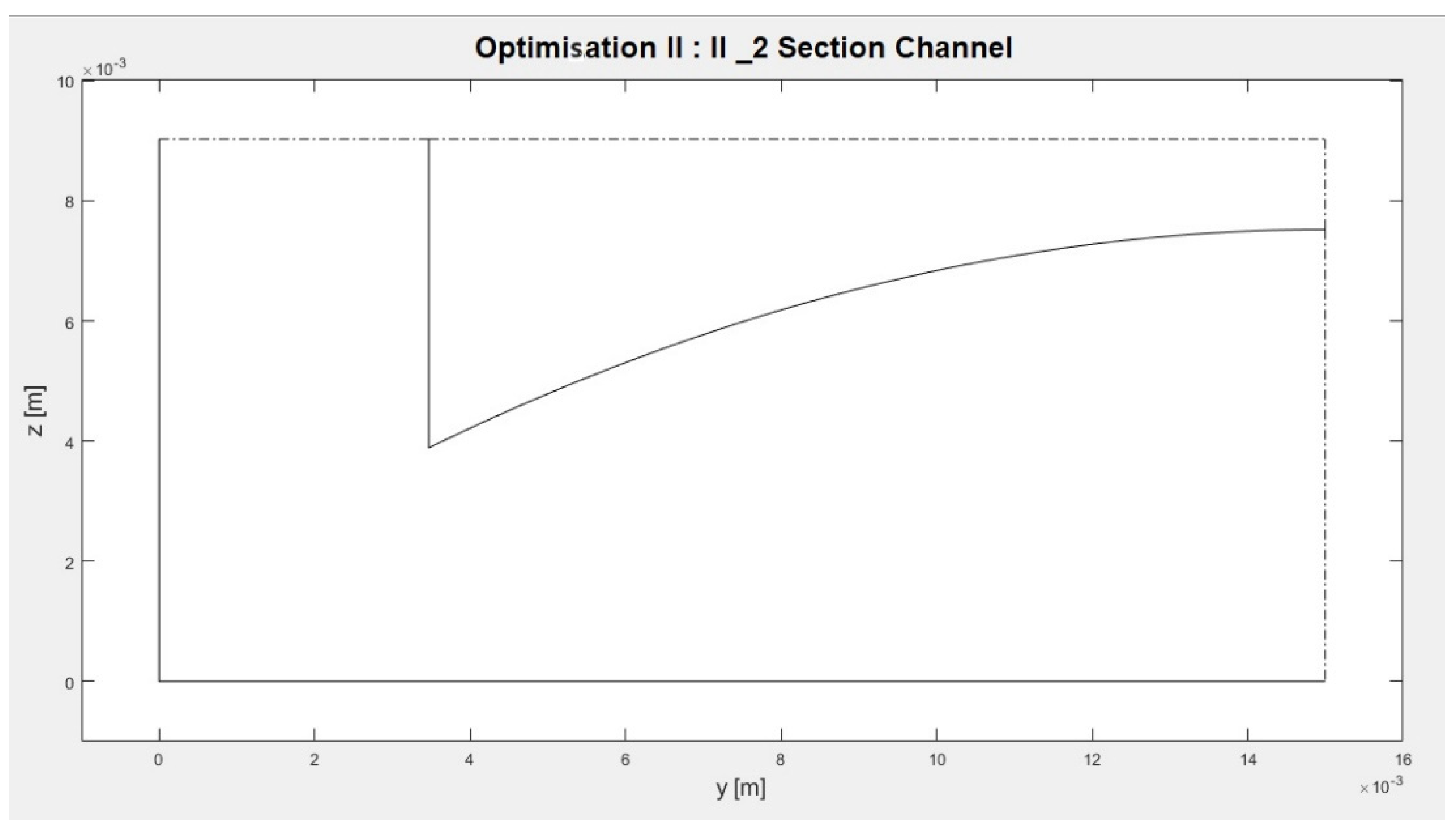
Optimization II-2: Type II optimization of a type A channel, with polynomial degree of the channel wall, n = 2;

-

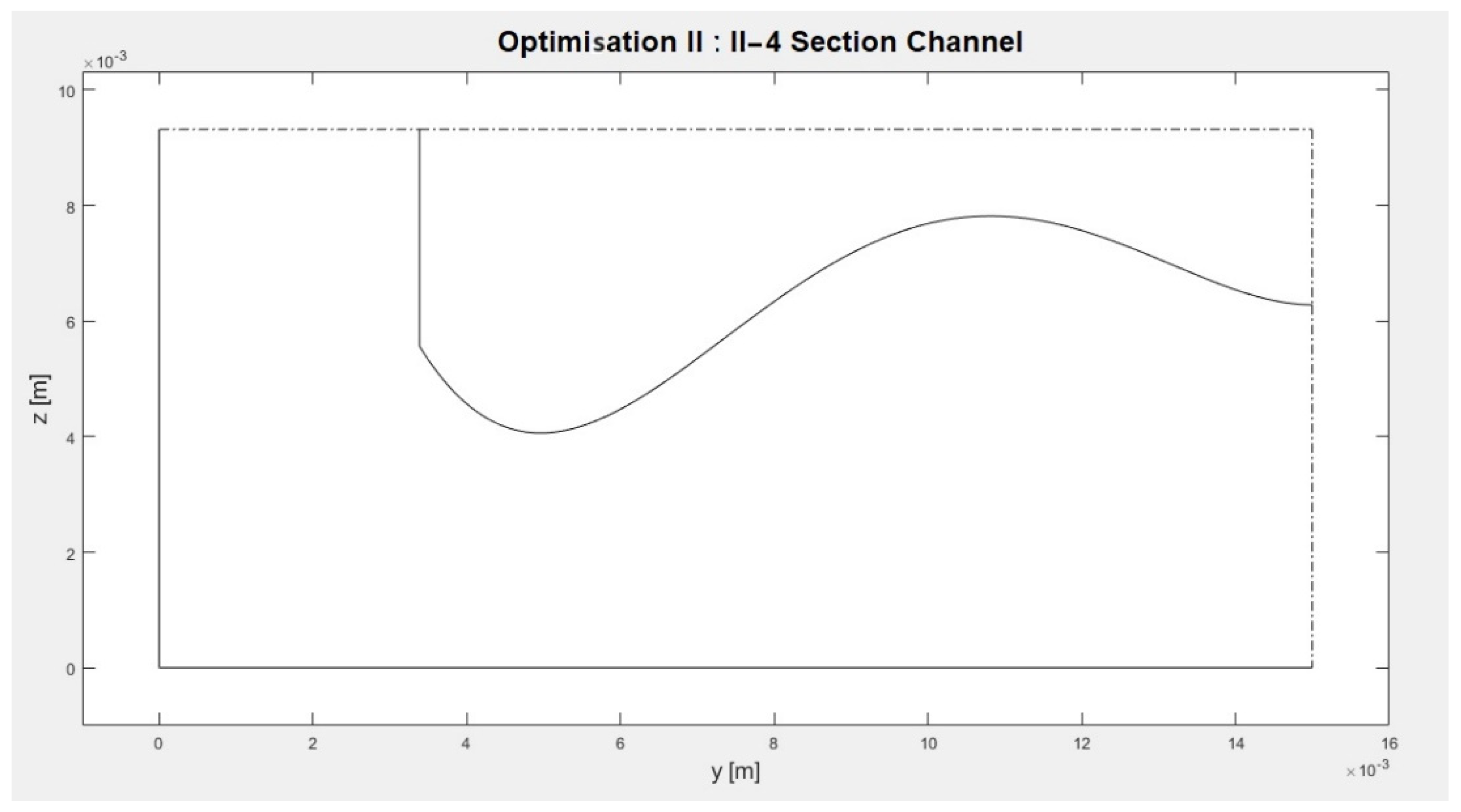
Optimization II-4: Type II optimization of a type A channel, with polynomial degree of the channel wall, n = 4.

Optimization II-2: channel A

The geometry of the channel obtained through optimization II-2 is depicted in Figure 14.

And it is described by the following parameters described in

Table 5. Channel A: section parameters (II-2).

${\mathrm{z}}_{\mathrm{p}2}\left[\mathrm{m}\right]$	${\mathrm{z}}_{\mathrm{p}1}\left[\mathrm{m}\right]$	${\mathrm{L}}_{\mathrm{z}}\left[\mathrm{m}\right]$	${\mathrm{L}}_{\mathrm{y}2}\left[\mathrm{m}\right]$	${\mathrm{L}}_{\mathrm{y}1}\left[\mathrm{m}\right]$
$0.007521$	$0.003887$	$0.009026$	$0.011531$	$0.003469$
${\mathrm{V}}_{\mathrm{t}\mathrm{o}\mathrm{t}}\left[{\mathrm{m}}^3\right]$	${\mathrm{V}}_{\mathrm{s}\mathrm{l}}\left[{\mathrm{m}}^3\right]$		${\mathrm{V}}_{\mathrm{f}}\left[{\mathrm{m}}^3\right]$
$2.7061·{10}^{-5}$	$2.07942·{10}^{-5}$		$6.2672·{10}^{-6}$
${\mathrm{A}}_{\mathrm{t}\mathrm{o}\mathrm{t}}\left[{\mathrm{m}}^2\right]$	${\mathrm{A}}_{\mathrm{s}\mathrm{l}}\left[{\mathrm{m}}^2\right]$		${\mathrm{A}}_{\mathrm{f}}\left[{\mathrm{m}}^2\right]$
$1.3531·{10}^{-4}$	$1.0397·{10}^{-4}$		$3.1336·{10}^{-5}$
$\frac{{\mathrm{V}}_{\mathrm{s}\mathrm{l}}}{{\mathrm{V}}_{\mathrm{t}\mathrm{o}\mathrm{t}}}$			$\frac{{\mathrm{V}}_{\mathrm{f}}}{{\mathrm{V}}_{\mathrm{t}\mathrm{o}\mathrm{t}}}$
$0.7684$			$0.2316$

.

The velocity field is depicted in Figure 15.

${\dot{\mathrm{V}}}_{\mathrm{f}}\left[{\mathrm{m}}^3/\mathrm{s}\right]$	$\overline{\mathrm{u}}\left[\mathrm{m}/\mathrm{s}\right]$	${\mathrm{u}}_{\mathrm{m}\mathrm{a}\mathrm{x}}\left[\mathrm{m}/\mathrm{s}\right]$
$4.5959·{10}^{-7}$	$0.0147$	$0.0335$

The time course of the temperature field is qualitatively very similar to that of the channel given by Optimization II-4. The time trends of the energy density and thermal power density are shown in Figure 16a,b.

The values of the performance parameters are as follows.

${\mathrm{t}}_{{\mathrm{Q}}_{\mathrm{s}\mathrm{l}\mathrm{m}\mathrm{a}\mathrm{x}}99\%}\left[\mathrm{s}\right]$	${\mathrm{t}}_{{\mathrm{Q}}_{\mathrm{s}\mathrm{l}\mathrm{m}\mathrm{a}\mathrm{x}}90\%}\left[\mathrm{s}\right]$	${\mathrm{t}}_{{\mathrm{Q}}_{\mathrm{s}\mathrm{l}\mathrm{r}\mathrm{e}\mathrm{f}}}\left[\mathrm{s}\right]$
$781.96$	$539.42$	$415.2$

$$\frac{{\mathrm{Q}}_{\mathrm{s}\mathrm{l}\mathrm{m}\mathrm{a}\mathrm{x}}}{{\mathrm{V}}_{\mathrm{t}\mathrm{o}\mathrm{t}}}=1.3463·{10}^8 \mathrm{J}/{\mathrm{m}}^3$$

$$\frac{{\mathrm{Q}}_{\mathrm{s}\mathrm{l}\mathrm{r}\mathrm{e}\mathrm{f}}}{{\mathrm{V}}_{\mathrm{t}\mathrm{o}\mathrm{t}\mathrm{r}\mathrm{e}\mathrm{f}}}·\frac{{\mathrm{V}}_{\mathrm{t}\mathrm{o}\mathrm{t}}}{{\mathrm{Q}}_{\mathrm{s}\mathrm{l}\mathrm{m}\mathrm{a}\mathrm{x}}}=0.8121$$

$$\frac{{\left.{\overline{\dot{\mathrm{Q}}}}_{\mathrm{s}\mathrm{l}}\right|}_{\mathrm{t}={\mathrm{t}}_{{\mathrm{Q}}_{\mathrm{s}\mathrm{l}\mathrm{r}\mathrm{e}\mathrm{f}}}}}{{\mathrm{V}}_{\mathrm{t}\mathrm{o}\mathrm{t}}}=2.6333·{10}^5 \mathrm{W}/{\mathrm{m}}^3$$

$$\frac{{\left.{\overline{\dot{\mathrm{Q}}}}_{\mathrm{s}\mathrm{l}}\right|}_{\mathrm{t}={\mathrm{t}}_{{\mathrm{Q}}_{\mathrm{s}\mathrm{l}\mathrm{m}\mathrm{a}\mathrm{x}}90\%}}}{{\mathrm{V}}_{\mathrm{t}\mathrm{o}\mathrm{t}}}=2.2462·{10}^5 \mathrm{W}/{\mathrm{m}}^3$$

$$\frac{{\left.{\overline{\dot{\mathrm{Q}}}}_{\mathrm{s}\mathrm{l}}\right|}_{\mathrm{t}={\mathrm{t}}_{{\mathrm{Q}}_{\mathrm{s}\mathrm{l}\mathrm{m}\mathrm{a}\mathrm{x}}99\%}}}{{\mathrm{V}}_{\mathrm{t}\mathrm{o}\mathrm{t}}}=1.7045·{10}^5 \mathrm{W}/{\mathrm{m}}^3$$

Optimization II-4: channel A

The geometry and channel speed range obtained through optimization II-4 are shown sequentially in Figure 17 and Figure 18.

And it is described by the following parameters (

Table 6. Channel A: section parameters (II-4).

${\mathrm{z}}_{\mathrm{p}4}\left[\mathrm{m}\right]$	${\mathrm{z}}_{\mathrm{p}3}\left[\mathrm{m}\right]$	${\mathrm{z}}_{\mathrm{p}2}\left[\mathrm{m}\right]$	${\mathrm{z}}_{\mathrm{p}1}\left[\mathrm{m}\right]$	${\mathrm{L}}_{\mathrm{z}}\left[\mathrm{m}\right]$	${\mathrm{L}}_{\mathrm{y}2}\left[\mathrm{m}\right]$	${\mathrm{L}}_{\mathrm{y}1}\left[\mathrm{m}\right]$
$0.00628$	$0.007797$	$0.005606$	$0.005561$	$0.009318$	$0.011613$	$0.003386$
${\mathrm{V}}_{\mathrm{t}\mathrm{o}\mathrm{t}}\left[{\mathrm{m}}^3\right]$				${\mathrm{V}}_{\mathrm{s}\mathrm{l}}\left[{\mathrm{m}}^3\right]$	${\mathrm{V}}_{\mathrm{f}}\left[{\mathrm{m}}^3\right]$
$2.7954·{10}^{-5}$				$2.0831·{10}^{-5}$	$7.1229·{10}^{-6}$
${\mathrm{A}}_{\mathrm{t}\mathrm{o}\mathrm{t}}\left[{\mathrm{m}}^2\right]$				${\mathrm{A}}_{\mathrm{s}\mathrm{l}}\left[{\mathrm{m}}^2\right]$	${\mathrm{A}}_{\mathrm{f}}\left[{\mathrm{m}}^2\right]$
$1.3977·{10}^{-4}$				$1.0416·{10}^{-4}$	$3.5615\mathrm{e}·{10}^{-5}$
$\frac{{\mathrm{V}}_{\mathrm{s}\mathrm{l}}}{{\mathrm{V}}_{\mathrm{t}\mathrm{o}\mathrm{t}}}$				$\frac{{\mathrm{V}}_{\mathrm{f}}}{{\mathrm{V}}_{\mathrm{t}\mathrm{o}\mathrm{t}}}$
$0.7452$				$0.2548$

).

${\dot{\mathrm{V}}}_{\mathrm{f}}\left[{\mathrm{m}}^3/\mathrm{s}\right]$	$\overline{\mathrm{u}}\left[\mathrm{m}/\mathrm{s}\right]$	${\mathrm{u}}_{\mathrm{m}\mathrm{a}\mathrm{x}}\left[\mathrm{m}/\mathrm{s}\right]$
$5.7122·{10}^{-7}$	$0.0160$	$0.0347$

The time course of the temperature field is depicted in the following Figure 19, Figure 20, Figure 21, Figure 22, Figure 23 and Figure 24.

Unlike the reference channel, at the initial time, the sections furthest from the fluid inlet were still at a temperature close to the initial temperature, whereas, in the reference channel, they were already close to the maximum temperature. This is probably due to a lower average velocity of the optimized II-4 channel than that of the reference channel.

From the previous figures, it can be seen that the last nodes in each section of the domain to merge are in the vicinity of the co-ordinate point $\left({\mathrm{x}}_{\mathrm{s}\mathrm{e}\mathrm{z}},{\mathrm{L}}_{\mathrm{y}},0\right)$ or the co-ordinate $x$ of a generic section.

Meanwhile, in the reference channel, they were in the vicinity of the co-ordinate point $\left({\mathrm{x}}_{\mathrm{s}\mathrm{e}\mathrm{z}},\mathrm{0,0}\right)$. This phenomenon is probably mainly due to the shape of the polynomial channel wall, which, unlike the reference channel, has a distance with the point (x_sez,0,0) smaller than the distance with the point $\left({\mathrm{x}}_{\mathrm{s}\mathrm{e}\mathrm{z}},{\mathrm{L}}_{\mathrm{y}},0\right)$.

The time trends of energy density and thermal power density are depicted in Figure 25a,b.

Below, the most interesting performance parameters are shown.

${\mathrm{t}}_{{\mathrm{Q}}_{\mathrm{s}\mathrm{l}\mathrm{m}\mathrm{a}\mathrm{x}}99\%}\left[\mathrm{s}\right]$	${\mathrm{t}}_{{\mathrm{Q}}_{\mathrm{s}\mathrm{l}\mathrm{m}\mathrm{a}\mathrm{x}}90\%}\left[\mathrm{s}\right]$	${\mathrm{t}}_{{\mathrm{Q}}_{\mathrm{s}\mathrm{l}\mathrm{r}\mathrm{e}\mathrm{f}}}\left[\mathrm{s}\right]$
$711.66$	$488.42$	$402.68$

$$\frac{{\mathrm{Q}}_{\mathrm{s}\mathrm{l}\mathrm{m}\mathrm{a}\mathrm{x}}}{{\mathrm{V}}_{\mathrm{t}\mathrm{o}\mathrm{t}}}=1.3057·{10}^8 \mathrm{J}/{\mathrm{m}}^3$$

$$\frac{{\mathrm{Q}}_{\mathrm{s}\mathrm{l}\mathrm{r}\mathrm{e}\mathrm{f}}}{{\mathrm{V}}_{\mathrm{t}\mathrm{o}\mathrm{t}\mathrm{r}\mathrm{e}\mathrm{f}}}·\frac{{\mathrm{V}}_{\mathrm{t}\mathrm{o}\mathrm{t}}}{{\mathrm{Q}}_{\mathrm{s}\mathrm{l}\mathrm{m}\mathrm{a}\mathrm{x}}}=0.8373$$

$$\frac{{\left.{\overline{\dot{\mathrm{Q}}}}_{\mathrm{s}\mathrm{l}}\right|}_{\mathrm{t}={\mathrm{t}}_{{\mathrm{Q}}_{\mathrm{s}\mathrm{l}\mathrm{r}\mathrm{e}\mathrm{f}}}}}{{\mathrm{V}}_{\mathrm{t}\mathrm{o}\mathrm{t}}}=2.7151·{10}^5 \mathrm{W}/{\mathrm{m}}^3$$

$$\frac{{\left.{\overline{\dot{\mathrm{Q}}}}_{\mathrm{s}\mathrm{l}}\right|}_{\mathrm{t}={\mathrm{t}}_{{\mathrm{Q}}_{\mathrm{s}\mathrm{l}\mathrm{m}\mathrm{a}\mathrm{x}}90\%}}}{{\mathrm{V}}_{\mathrm{t}\mathrm{o}\mathrm{t}}}=2.4060·{10}^5 \mathrm{W}/{\mathrm{m}}^3$$

$$\frac{{\left.{\overline{\dot{\mathrm{Q}}}}_{\mathrm{s}\mathrm{l}}\right|}_{\mathrm{t}={\mathrm{t}}_{{\mathrm{Q}}_{\mathrm{s}\mathrm{l}\mathrm{m}\mathrm{a}\mathrm{x}}99\%}}}{{\mathrm{V}}_{\mathrm{t}\mathrm{o}\mathrm{t}}}=1.8164·{10}^5 \mathrm{W}/{\mathrm{m}}^3$$

The following figure (Figure 26a–d) show accumulated energy density evaluated for different section channel parameters.

4. Conclusions

The performed optimizations using a simple genetic algorithm provide significant improvements in the performance of the proposed polynomial profile wall PCM heat storage system. However, it is difficult to distinguish with certainty whether the results obtained are, in fact, absolute maxima (or minima) at a mathematical level. Given the results of optimizations N-2-4, this hypothesis is unlikely, but further analysis is required to draw conclusions on this point. The results of optimizations 2, 4, and 2-4, belonging to the same N-optimization, gave quite comparable results to each other and significantly better than the reference profile. With regard to optimizations I and II all having the same evaluation parameters, we can state that the one that gave the best results was optimization I because it was the one with the least restrictive conditions among the three and, therefore, with the greatest possibility of variation in the channel geometry. Meanwhile the one with the worst results is optimization II because of the most restrictive conditions, i.e., constant solid/liquid volume. The performance of channel B was compared with that of channel A with the same geometry. A metal frame increases the surface area by 6.

References

- Kumar, R.; Rao, Y.A.; Yadav, A.S.; Balu, A.; Panda, B.P.; Joshi, M.; Taneja, S.; Sharma, A. Application of phase change material in thermal energy storage systems. Mater. Today Proc. 2022, 63, 798–804. [Google Scholar] [CrossRef]
- Vakilaltojjar, S.M.; Saman, W. Analysis and modelling of a phase change storage system for air conditioning applications. Appl. Therm. Eng. 2001, 21, 249–263. [Google Scholar] [CrossRef]
- Marín, J.M.; Zalba, B.; Cabeza, L.F.; Mehling, H. Improvement of a thermal energy storage using plates with paraffin–graphite composite. Int. J. Heat Mass Transf. 2005, 48, 2561–2570. [Google Scholar] [CrossRef]
- Cabeza, L.; Mehling, H.; Hiebler, S.; Ziegler, F. Heat transfer enhancement in water when used as PCM in thermal energy storage. Appl. Therm. Eng. 2002, 22, 1141–1151. [Google Scholar] [CrossRef]
- Mehling, H.; Hiebler, S.; Ziegler, F. Latent heat storage using a PCM–graphite composite material. In Proceedings of the Terrastock 2000—8th International Conference on Thermal Energy Storage, Stuttgart, Germany, 28 August–1 September 2000; pp. 375–380. [Google Scholar]
- Py, X.; Olives, R.; Mauran, S. Paraffin/porous-graphite-matrix composite as a high and constant power thermal storage material. Int. J. Heat Mass Transf. 2001, 44, 2727–2737. [Google Scholar] [CrossRef]
- Xiao, M.; Feng, B.; Gong, K. Thermal performance of a high conductive shape-stabilized thermal storage material. Sol. Energy Mater. Sol. Cells 2001, 69, 293–296. [Google Scholar] [CrossRef]
- Wang, W.; Yang, X.; Fang, Y.; Ding, J. Preparation and performance of form-stable polyethylene glycol/silicon dioxide composites as solid–liquid phase change materials. Appl. Energy 2008, 86, 170–174. [Google Scholar] [CrossRef]
- Wang, W.; Yang, X.; Fang, Y.; Ding, J.; Yan, J. Enhanced thermal conductivity and thermal performance of form-stable composite phase change materials by using ß-aluminum nitride. Appl. Energy 2009, 86, 1196–1200. [Google Scholar] [CrossRef]
- Ismail, K.; Alves, C.; Modesto, M. Numerical and experimental study on the solidification of PCM around a vertical axially finned isothermal cylinder. Appl. Therm. Eng. 2001, 21, 53–77. [Google Scholar] [CrossRef]
- Stritih, U. An experimental study of enhanced heat transfer in rectangular PCM thermal storage. Int. J. Heat Mass Transf. 2004, 47, 2841–2847. [Google Scholar] [CrossRef]
- Trp, A. An experimental and numerical investigation of heat transfer during technical grade paraffin melting and solidification in a shell-and-tube latent thermal energy storage unit. Sol. Energy 2005, 79, 648–660. [Google Scholar] [CrossRef]
- Trp, A.; Lenic, K.; Frankovic, B. Analysis of the influence of operating conditions and geometric parameters on heat transfer in water-paraffin shell-and-tube latent thermal energy storage unit. Appl. Therm. Eng. 2006, 26, 1830–1839. [Google Scholar] [CrossRef]
- Erek, A.; Ilken, Z.; Acar, M.A. Experimental and numerical investigation of thermal energy storage with a finned tube. Int. J. Energy Res. 2005, 29, 283–301. [Google Scholar] [CrossRef]
- Erek, A.; Ezan, M.A. Experimental and numerical study on charging processes of an ice-on-coil thermal energy storage system. Int. J. Energy Res. 2007, 31, 158–176. [Google Scholar] [CrossRef]
- Zalba, B. Free Cooling, an Application of PCMs in TES. Ph.D. Thesis, University of Zaragoza, Zaragoza, Spain, 2002. [Google Scholar]
- Bagley, J.D. The Behavior of Adaptive Systems Which Employ Genetic and Correlation Algorithms. Ph.D. Thesis, University of Michigan, Ann Arbor, MI, USA, 1967. [Google Scholar]
- De Jong, K.A. An analysis of the behavior of a class of genetic adaptive systems. Diss. Abstr. Int. 1975, 36, 5140B. [Google Scholar]
- Grefenstette, J.J. Optimization of control parameters for genetic algorithms. IEEE Trans. Syst. Man Cybern. 1986, 16, 122–128. [Google Scholar] [CrossRef]
- Queipo, N.; Devarakonda, R.; Humphrey, J. Genetic algorithms for thermosciences research: Application to the optimized cooling of electronic components. Int. J. Heat Mass Transf. 1994, 37, 893–908. [Google Scholar] [CrossRef]
- Fabbri, G. A genetic algorithm for fin profile optimization. Int. J. Heat Mass Transf. 1997, 40, 2165–2172. [Google Scholar] [CrossRef]
- Selbaş, R.; Kızılkan, O.; Reppich, M. A new design approach for shell-and-tube heat exchangers using genetic algorithms from economic point of view. Chem. Eng. Process.—Process Intensif. 2005, 45, 268–275. [Google Scholar] [CrossRef]
- Lu, L.; Cai, W.J.; Chai, Y.S.; Xie, L. Global optimization for overall HVAC systems—Part I problem ormulation and analysis. Energy Convers. Manag. 2005, 46, 999–1014. [Google Scholar] [CrossRef]
- Lu, L.; Cai, W.; Soh, Y.C.; Xie, L. Global optimization for overall HVAC systems—Part II problem solution and simulations. Energy Convers. Manag. 2004, 46, 1015–1028. [Google Scholar] [CrossRef]
- Atashkari, K.; Nariman-Zadeh, N.; Pilechi, A.; Jamali, A.; Yao, X. Thermodynamic Pareto optimization of turbojet engines using multi-objective genetic algorithms. Int. J. Therm. Sci. 2005, 44, 1061–1071. [Google Scholar] [CrossRef]
- Zhou, H.; Cen, K.; Fan, J. Multi-objective optimization of the coal combustion performance with artificial neural networks and genetic algorithms. Int. J. Energy Res. 2005, 29, 499–510. [Google Scholar] [CrossRef]
- Gosselin, L.; Tye-Gingras, M.; Mathieu-Potvin, F. Review of utilization of genetic algorithms in heat transfer problems. Int. J. Heat Mass Transf. 2009, 52, 2169–2188. [Google Scholar] [CrossRef]
- Fabbri, G.; Greppi, M.; Amati, F. Numerical Analysis of New PCM Thermal Storage Systems. Energies 2024, 17, 1772. [Google Scholar] [CrossRef]