


Multiphase Flow’s Volume Fractions Intelligent Measurement by a Compound Method Employing Cesium-137, Photon Attenuation Sensor, and Capacitance-Based Sensor

 ,
,  , , and
Abstract
1. Introduction
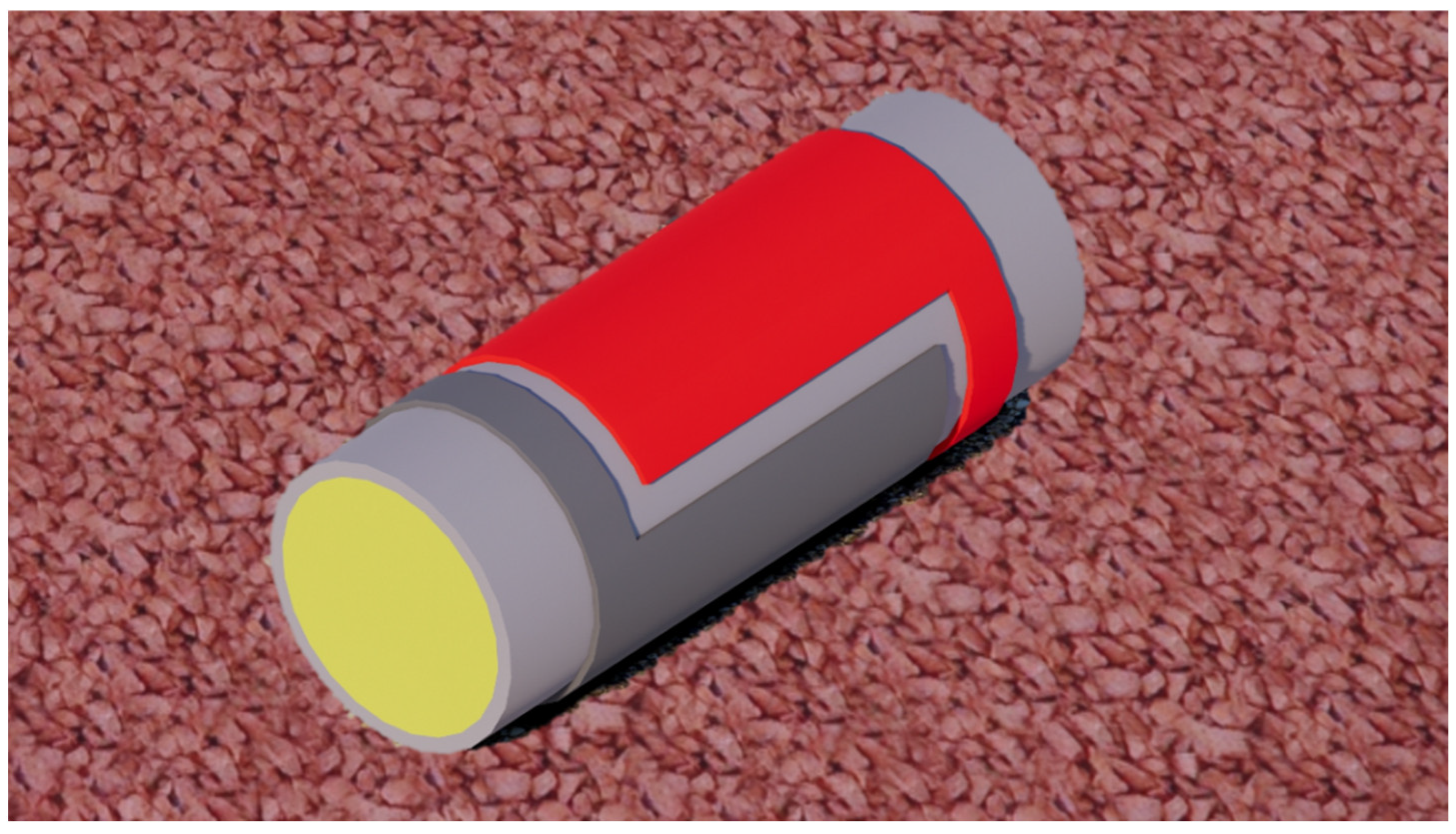
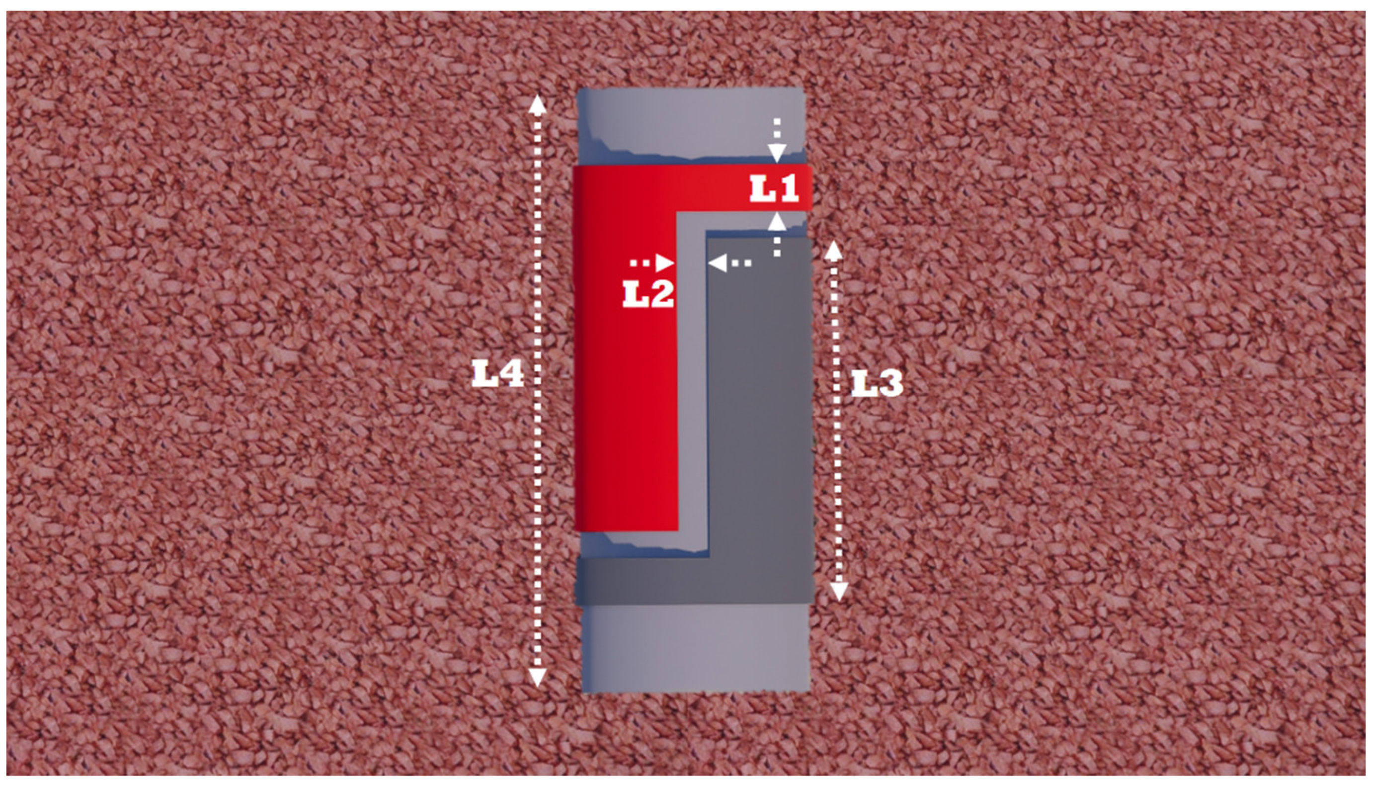
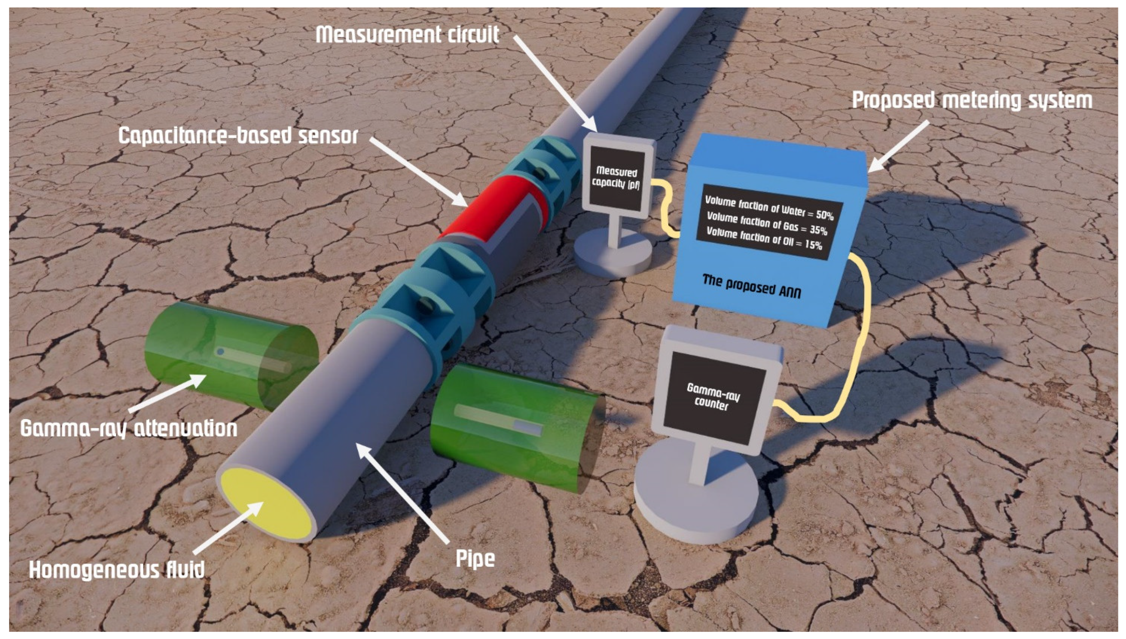
2. The Employed Sensors

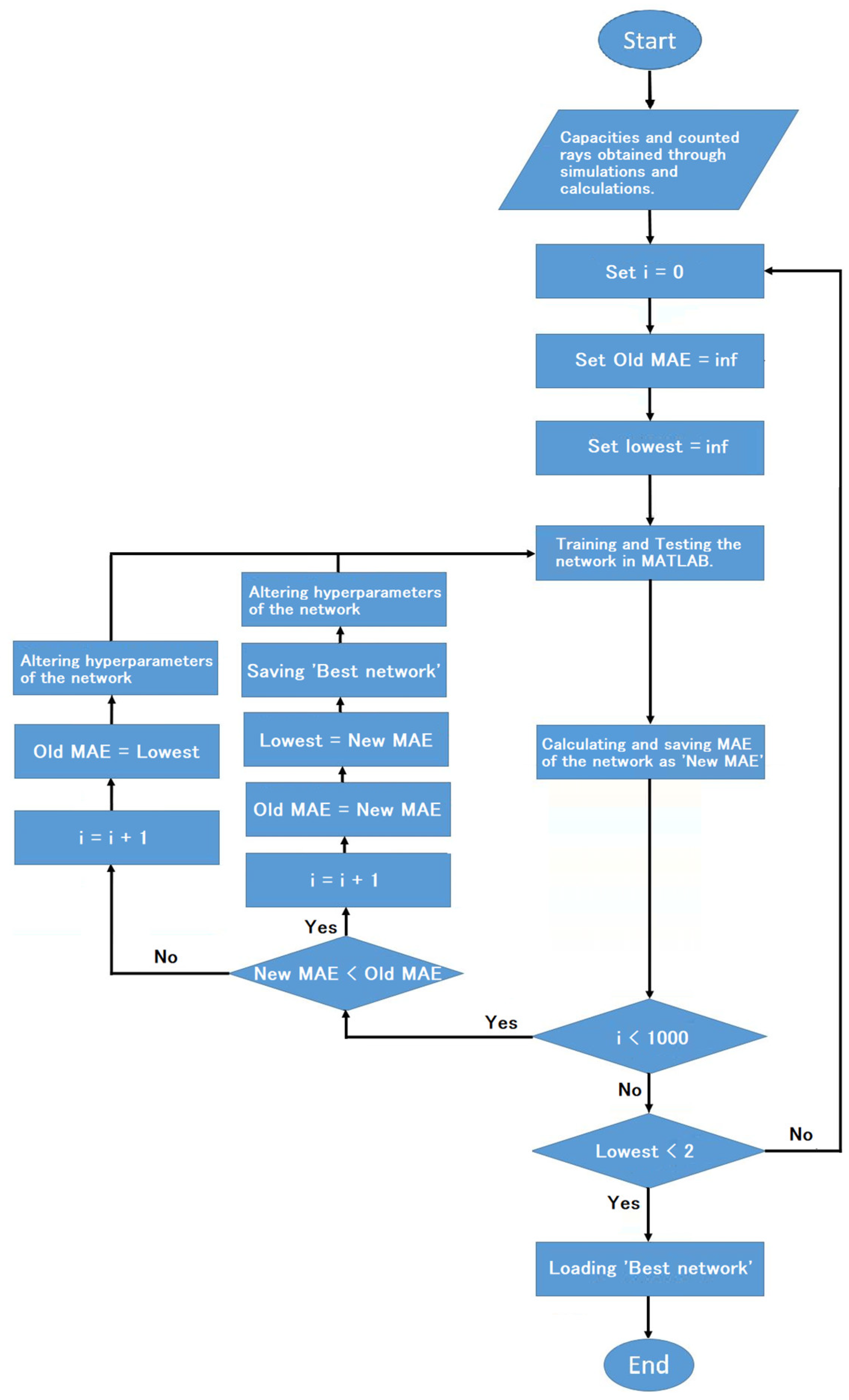
3. Artificial Neural Network
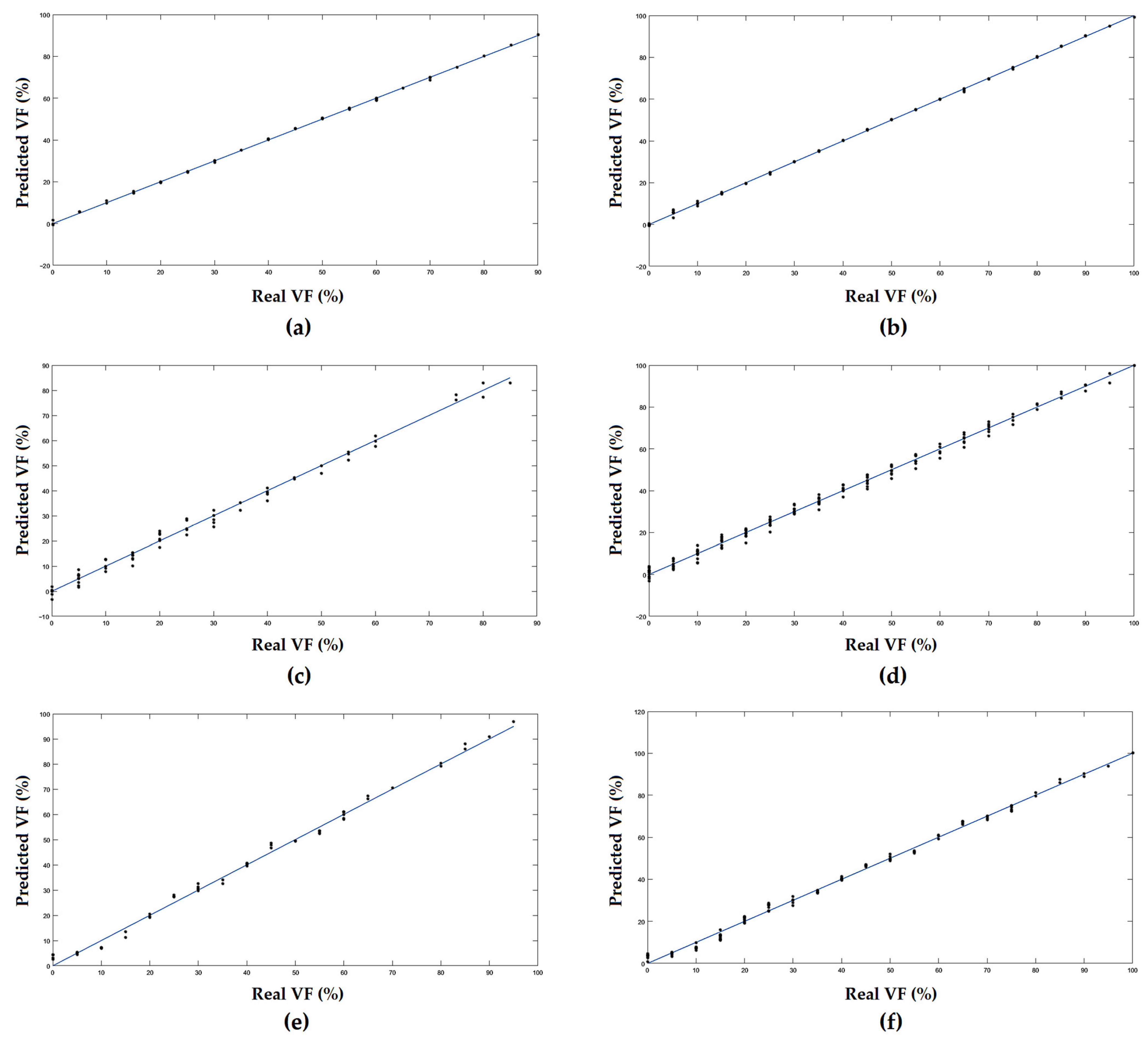
4. Results and Discussion
5. Conclusions
Author Contributions
Funding
Data Availability Statement
Conflicts of Interest
References
- Chen, X.; Chen, L.; Zhou, F.; Lin, F. Crude Oil/Natural gas/Water Three-Phase Flow meter. In Proceedings of the SPE, 63rd Annual Technical Conference and Exhibition of the Society of Petroleum Engineers, Houston, TX, USA, 2–5 October 1988. [Google Scholar]
- Thorn, R.; Johansen, G.A.; Hammer, E.A. Recent developments in three-phase flow measurement. Meas. Sci. Technol. 1997, 8, 691. [Google Scholar] [CrossRef]
- Thorn, R.; Johansen, G.A.; Hjertaker, B.T. Three-phase flow measurement in the petroleum industry. Meas. Sci. Technol. 2012, 24, 012003. [Google Scholar] [CrossRef]
- Huang, S.M.; Plaskowski, A.B.; Xie, C.G.; Beck, M.S. Capacitance-based tomographic flow imaging system. Electron Lett. 1988, 24, 418. [Google Scholar] [CrossRef]
- Liu, S.; Chen, Q.; Wang, H.G.; Jiang, F.; Ismail, I.; Yang, W.Q. Electrical capacitance tomography for gas–solids flow measurement for circulating fluidized beds. Flow Meas. Instrum. 2005, 16, 135–144. [Google Scholar] [CrossRef]
- Hossain, M.S.; Abir, M.T.; Alam, M.S.; Volakis, J.L.; Islam, M.A. An algorithm to image individual phase fractions of multiphase flows using electrical capacitance tomography. IEEE Sens. J. 2020, 20, 14924–14931. [Google Scholar] [CrossRef]
- Dias, F.D.; dos Santos, E.N.; da Silva, M.J.; Schleicher, E.; Morales, R.E.; Hewakandamby, B.; Hampel, U. New algorithm to discriminate phase distribution of gas-oil-water pipe flow with dual-modality wire-mesh sensor. IEEE Access 2020, 8, 125163–125178. [Google Scholar] [CrossRef]
- Isaksen, O. Three Phase Pipe Flow Imaging Using a Capacitance Tomography System. In Proceedings of the IEE Colloquium on Advances in Sensors for Fluid Flow Measurements, London, UK, 18 April 1996; pp. 11/1–11/6. [Google Scholar]
- Qu, Z.; Zhao, Q.; Meng, Y. On oil measurement of water concentration of oil-water mixture in the flow of pipeline by using eddy current. J. Meas. Sci. Technol. 2012, 24, 125304. [Google Scholar] [CrossRef]
- Sheikh, S.I.; Al-Quraish, K.; Ragheb, H.A.; Babelli, I. Simple Microwave Method for Detecting Water Holdup. Microw. Opt. Technol. Lett. 2008, 50, 354–355. [Google Scholar] [CrossRef]
- Libert, N.; Da Silva, M.J. Capacitive measuring system for two-phase flow monitoring. Part 1: Hardware design and evaluation. Flow Meas. Instrum. 2016, 47, 90–99. [Google Scholar] [CrossRef]
- Yang, D.; Pu, H.; Han, H.; Liu, L.; Yan, C. Huge-scale capacitance mass flowmeter in gas/solid two-phase flow with rectangular vertical pipeline. Measurement 2020, 151, 107235. [Google Scholar] [CrossRef]
- Salgado, C.M.; Pereira, C.M.; Schirru, R.; Brandão, L.E. Flow regime identification and volume fraction prediction in multiphase flows by means of gamma-ray attenuation and artificial neural networks. Prog. Nucl. Energy 2010, 52, 555–562. [Google Scholar] [CrossRef]
- Salgado, W.L.; Dam, R.S.; Salgado, C.M. Optimization of a flow regime identification system and prediction of volume fractions in three-phase systems using gamma-rays and artificial neural network. Appl. Radiat. Isot. 2021, 169, 109552. [Google Scholar] [CrossRef] [PubMed]
- Roshani, G.; Karami, A.; Salehizadeh, A.; Nazemi, E. The capability of radial basis function to forecast the volume fractions of the annular three-phase flow of gas-oil-water. Appl. Radiat. Isot. 2017, 129, 156–162. [Google Scholar] [CrossRef] [PubMed]
- Chen, T.-C.; Alizadeh, S.M.; Alanazi, A.K.; Grimaldo Guerrero, J.W.; Abo-Dief, H.M.; Eftekhari-Zadeh, E.; Fouladinia, F. Using ANN and Combined Capacitive Sensors to Predict the Void Fraction for a Two-Phase Homogeneous Fluid Independent of the Liquid Phase Type. Processes 2023, 11, 940. [Google Scholar] [CrossRef]
- Qaisi, R.M.; Fouladinia, F.; Mayet, A.M.; Guerrero, J.W.; Loukil, H.; Raja, M.R.; Muqeet, M.A.; Eftekhari-Zadeh, E. Intelligent measuring of the volume fraction considering temperature changes and independent pressure variations for a two-phase homogeneous fluid using an 8-electrode sensor and an ANN. Sensors 2023, 23, 6959. [Google Scholar] [CrossRef] [PubMed]
- Syah, R.B.Y.; Veisi, A.; Hasibuan, Z.A.; Al-Fayoumi, M.A.; Daoud, M.S. A Novel Smart Optimized Capacitance-Based Sensor for Annular Two-Phase Flow Metering with High Sensitivity. IEEE Access 2023, 11, 60709–60716. [Google Scholar] [CrossRef]
- Ribeiro, J.X.; Liao, R.; Aliyu, A.M.; Liu, Z. Prediction of pressure gradient in two and three-phase flows in vertical pipes using an artificial neural network model. Int. J. Eng. Technol. Innov. 2019, 9, 155–170. [Google Scholar]
- Roshani, G.H.; Muhammad Ali, P.J.; Mohammed, S.; Hanus, R.; Abdulkareem, L.; Alanezi, A.A.; Nazemi, E.; Eftekhari-Zadeh, E.; Kalmoun, E.M. Feasibility study of using X-ray tube and GMDH for measuring volume fractions of annular and stratified regimes in three-phase flows. Symmetry 2021, 13, 613. [Google Scholar] [CrossRef]
- Peyvandi, R.G.; Rad, S.Z.I. Application of artificial neural networks for the prediction of volume fraction using spectra of gammarays backscattered by three-phase flows. Eur. Phys. J. Plus 2017, 132, 511. [Google Scholar] [CrossRef]
- Mayet, A.M.; Fouladinia, F.; Alizadeh, S.M.; Alhashim, H.H.; Guerrero, J.W.; Loukil, H.; Parayangat, M.; Nazemi, E.; Shukla, N.K. Measuring volume fractions of a three-phase flow without separation utilizing an approach based on artificial intelligence and capacitive sensors. PLoS ONE 2024, 19, e0301437. [Google Scholar] [CrossRef] [PubMed]
- Falcone, G. Key multiphase flow metering techniques. Dev. Pet. Sci. 2009, 54, 47–190. [Google Scholar]
- Fouladinia, F.; Alizadeh, S.M.; Gorelkina, E.I.; Hameed Shah, U.; Nazemi, E.; Guerrero, J.W.G.; Roshani, G.H.; Imran, A. A novel metering system consists of capacitance-based sensor, gamma-ray sensor and ANN for measuring volume fractions of three-phase homogeneous flows. Nondestruct. Test. Eval. 2024, 8, 1–27. [Google Scholar] [CrossRef]
- Terzic, E.; Terzic, J.; Nagarajah, R.; Alamgir, M.; Terzic, E.; Terzic, J.; Nagarajah, R.; Alamgir, M. Capacitive sensing technology. In A Neural Network Approach to Fluid Quantity Measurement in Dynamic Environments; Springer: London, UK, 2012; pp. 11–37. [Google Scholar]
- Salehi, S.M.; Karimi, H.; Dastranj, A.A.; Moosavi, R. Twin rectangular fork-like capacitance sensor to flow regime identification in horizontal co-current gas–liquid two-phase flow. IEEE Sens. J. 2017, 17, 4834–4842. [Google Scholar] [CrossRef]
- Iliyasu, A.M.; Fouladinia, F.; Salama, A.S.; Roshani, G.H.; Hirota, K. Intelligent Measurement of Void Fractions in Homogeneous Regime of Two-Phase Flows Independent of the Liquid Phase Density Changes. Fractal Fract. 2023, 7, 179. [Google Scholar] [CrossRef]
- Li, D.H.; Wu, Y.X.; Li, Z.B.; Zhong, X.F. Volumetric fraction measurement in oil-water-gas multiphase flow with dual energy gamma-ray system. J. Zhejiang Univ. Sci. A 2005, 6, 1405–1411. [Google Scholar]
- Available online: https://physics.nist.gov/PhysRefData/Xcom/html/xcom1.html (accessed on 20 February 2024).
- Esteva, A.; Robicquet, A.; Ramsundar, B.; Kuleshov, V.; DePristo, M.; Chou, K.; Cui, C.; Corrado, G.; Thrun, S.; Dean, J. A guide to deep learning in healthcare. Nat. Med. 2019, 25, 24–29. [Google Scholar] [CrossRef] [PubMed]
- Gallant, A.R.; White, H. On learning the derivatives of an unknown mapping with multilayer feedforward networks. Neural Netw. 1992, 5, 129–138. [Google Scholar] [CrossRef]
- Salgado, C.M.; Brandão, L.E.; Schirru, R.; Pereira, C.M.; da Silva, A.X.; Ramos, R. Prediction of volume fractions in three-phase flows using nuclear technique and artificial neural network. Appl. Radiat. Isot. 2009, 67, 1812–1818. [Google Scholar] [CrossRef] [PubMed]
- Marquardt, D.W. An algorithm for least-squares estimation of nonlinear parameters. J. Soc. Ind. Appl. Math. 1963, 11, 431–441. [Google Scholar] [CrossRef]
- Levenberg, K. A method for the solution of certain non-linear problems in least squares. Q. Appl. Math. 1944, 2, 164–168. [Google Scholar] [CrossRef]
- Salgado, C.M.; Brandão, L.E.; Conti, C.C.; Salgado, W.L. Density prediction for petroleum and derivatives by gamma-ray attenuation and artificial neural networks. Appl. Radiat. Isot. 2016, 116, 143–149. [Google Scholar] [CrossRef] [PubMed]
- Engineering ToolBox. 2001. Available online: https://www.engineeringtoolbox.com (accessed on 1 July 2024).
- Roshani, M.; Phan, G.; Roshani, G.H.; Hanus, R.; Nazemi, B.; Corniani, E.; Nazemi, E. Combination of X-ray tube and GMDH neural network as a nondestructive and potential technique for measuring characteristics of gas-oil–water three phase flows. Measurement 2021, 168, 108427. [Google Scholar] [CrossRef]
- Pan, Y.; Li, C.; Ma, Y.; Huang, S.; Wang, D. Gas flow rate measurement in low-quality multiphase flows using Venturi and gamma ray. Exp. Therm. Fluid Sci. 2019, 100, 319–327. [Google Scholar] [CrossRef]
- Taylan, O.; Sattari, M.A.; Elhachfi Essoussi, I.; Nazemi, E. Frequency domain feature extraction investigation to increase the accuracy of an intelligent nondestructive system for volume fraction and regime determination of gas-water-oil three-phase flows. Mathematics 2021, 9, 2091. [Google Scholar] [CrossRef]
- Roshani, G.H.; Nazemi, E.; Roshani, M.M. Intelligent recognition of gas-oil-water three-phase flow regime and determination of volume fraction using radial basis function. Flow Meas. Instrum. 2017, 54, 39–45. [Google Scholar] [CrossRef]


| Gas | Water | Oil | |
|---|---|---|---|
| (kg/m3) | 1.2 | 1000 | 900 |
| (Pa·s) | 1.8 × | 0.001 | 0.5 |
| (W/m·K) | 0.025 | 0.6 | 0.15 |
| (J/kg·K) | 1005 | 4186 | 2000 |
| Gas VF Real (%) | Water VF Real (%) | Oil VF Real (%) | Gas VF Predicted (%) | Water VF Predicted (%) | Oil VF Predicted (%) | Gas’s Absolute | Water’s Absolute | Oil’s Absolute |
|---|---|---|---|---|---|---|---|---|
| Error | Error | Error | ||||||
| 15 | 85 | 0 | 10.913387 | 85.172807 | 3.9137882 | 4.086613 | 0.172807 | 3.913788 |
| 25 | 65 | 10 | 27.831509 | 64.736502 | 7.4319771 | 2.831509 | 0.263498 | 2.568023 |
| 10 | 30 | 60 | 7.7712042 | 29.838744 | 62.390046 | 2.228796 | 0.161256 | 2.390046 |
| 25 | 10 | 65 | 26.572223 | 10.069296 | 63.35853 | 1.572223 | 0.069296 | 1.64147 |
| 50 | 25 | 25 | 49.243431 | 24.776412 | 25.980178 | 0.756569 | 0.223588 | 0.980178 |
| 15 | 75 | 10 | 11.285484 | 74.959631 | 13.754864 | 3.714516 | 0.040369 | 3.754864 |
| 65 | 10 | 25 | 66.884093 | 9.8224062 | 23.293635 | 1.884093 | 0.177594 | 1.706365 |
| 80 | 5 | 15 | 79.665931 | 6.5701996 | 13.76407 | 0.334069 | 1.5702 | 1.23593 |
| 35 | 25 | 40 | 33.933778 | 24.887602 | 41.178638 | 1.066222 | 0.112398 | 1.178638 |
| 5 | 50 | 45 | 5.0178017 | 50.138509 | 44.843658 | 0.017802 | 0.138509 | 0.156342 |
| 5 | 75 | 20 | 5.3384456 | 75.086652 | 19.574875 | 0.338446 | 0.086652 | 0.425125 |
| 5 | 65 | 30 | 5.0679691 | 64.860442 | 30.071558 | 0.067969 | 0.139558 | 0.071558 |
| 0 | 10 | 90 | 2.6335723 | 9.7371359 | 87.629322 | 2.633572 | 0.262864 | 2.370678 |
| 35 | 35 | 30 | 33.488231 | 35.269481 | 31.242289 | 1.511769 | 0.269481 | 1.242289 |
| 20 | 55 | 25 | 19.276919 | 55.168548 | 25.554513 | 0.723081 | 0.168548 | 0.554513 |
| 35 | 30 | 35 | 33.714687 | 30.08246 | 36.202862 | 1.285313 | 0.08246 | 1.202862 |
| 10 | 35 | 55 | 7.6975647 | 35.02615 | 57.276271 | 2.302435 | 0.02615 | 2.276271 |
| 70 | 15 | 15 | 69.620939 | 14.709692 | 15.669506 | 0.379061 | 0.290308 | 0.669506 |
| 35 | 15 | 50 | 33.890651 | 14.758431 | 51.350955 | 1.109349 | 0.241569 | 1.350955 |
| 85 | 5 | 10 | 87.404505 | 7.0362529 | 5.5594775 | 2.404505 | 2.036253 | 4.440522 |
| 35 | 45 | 20 | 33.344459 | 45.387005 | 21.268525 | 1.655541 | 0.387005 | 1.268525 |
| 10 | 85 | 5 | 6.876399 | 85.331049 | 7.7925308 | 3.123601 | 0.331049 | 2.792531 |
| 20 | 35 | 45 | 21.064888 | 35.260079 | 43.67503 | 1.064888 | 0.260079 | 1.32497 |
| 25 | 75 | 0 | 28.738268 | 74.392027 | −3.1303018 | 3.738268 | 0.607973 | 3.130302 |
| 5 | 95 | 0 | 3.350574 | 94.952338 | 1.6970701 | 1.649426 | 0.047662 | 1.69707 |
| 80 | 0 | 20 | 81.056923 | −0.5433485 | 19.486638 | 1.056923 | 0.543349 | 0.513363 |
| 100 | 0 | 0 | 100.25363 | 0.5660806 | −0.8194028 | 0.253631 | 0.566081 | 0.819403 |
| 0 | 5 | 95 | 3.000451 | 5.3820733 | 91.617517 | 3.000451 | 0.382073 | 3.382483 |
| 5 | 5 | 90 | 4.3715126 | 5.3609461 | 90.267584 | 0.628487 | 0.360946 | 0.267584 |
| 10 | 40 | 50 | 7.5304801 | 40.15452 | 52.314979 | 2.46952 | 0.15452 | 2.314979 |
| 75 | 25 | 0 | 74.797941 | 24.062943 | 1.1392578 | 0.202059 | 0.937057 | 1.139258 |
| 15 | 10 | 75 | 13.620304 | 9.8520346 | 76.527701 | 1.379696 | 0.147965 | 1.527701 |
| 5 | 45 | 50 | 5.1056063 | 45.211362 | 49.683004 | 0.105606 | 0.211362 | 0.316996 |
| 45 | 5 | 50 | 46.677298 | 5.5768348 | 47.74592 | 1.677298 | 0.576835 | 2.25408 |
| 60 | 20 | 20 | 60.454517 | 19.662207 | 19.883359 | 0.454517 | 0.337793 | 0.116641 |
| 20 | 70 | 10 | 19.071512 | 69.797086 | 11.131384 | 0.928488 | 0.202914 | 1.131384 |
| 50 | 20 | 30 | 49.287898 | 19.646974 | 31.06516 | 0.712102 | 0.353026 | 1.06516 |
| 30 | 50 | 20 | 30.288257 | 50.342381 | 19.36935 | 0.288257 | 0.342381 | 0.63065 |
| 60 | 30 | 10 | 59.157734 | 29.953677 | 10.888646 | 0.842266 | 0.046323 | 0.888646 |
| 20 | 0 | 80 | 21.2667 | −0.088374 | 78.821723 | 1.2667 | 0.088374 | 1.178277 |
| 10 | 90 | 0 | 6.2338835 | 90.251039 | 3.5150582 | 3.766117 | 0.251039 | 3.515058 |
| 40 | 30 | 30 | 39.879803 | 30.037108 | 30.083096 | 0.120198 | 0.037108 | 0.083096 |
| 65 | 20 | 15 | 67.472182 | 19.671555 | 12.85638 | 2.472182 | 0.328445 | 2.14362 |
| 5 | 0 | 95 | 4.4833565 | −0.4718652 | 95.988546 | 0.516644 | 0.471865 | 0.988546 |
| 40 | 25 | 35 | 40.200223 | 24.853591 | 34.946202 | 0.200223 | 0.146409 | 0.053798 |
| 50 | 0 | 50 | 48.684902 | −0.041292 | 51.35646 | 1.315098 | 0.041292 | 1.35646 |
| 45 | 25 | 30 | 46.440611 | 24.823834 | 28.73557 | 1.440611 | 0.176166 | 1.26443 |
| 20 | 30 | 50 | 21.610296 | 30.087453 | 48.302256 | 1.610296 | 0.087453 | 1.697744 |
| 40 | 0 | 60 | 41.383771 | −0.0013561 | 58.617638 | 1.383771 | 0.001356 | 1.382362 |
| 0 | 50 | 50 | 4.1279189 | 50.192889 | 45.679161 | 4.127919 | 0.192889 | 4.320839 |
| 35 | 20 | 45 | 34.029008 | 19.763423 | 46.207596 | 0.970992 | 0.236577 | 1.207596 |
| 65 | 0 | 35 | 65.993002 | −0.3015169 | 34.308578 | 0.993002 | 0.301517 | 0.691422 |
| 5 | 15 | 80 | 4.0333148 | 14.485203 | 81.481503 | 0.966685 | 0.514797 | 1.481503 |
| 10 | 50 | 40 | 7.140987 | 50.134776 | 42.724208 | 2.859013 | 0.134776 | 2.724208 |
| 20 | 20 | 60 | 22.287136 | 19.79164 | 57.921249 | 2.287136 | 0.20836 | 2.078751 |
| 20 | 5 | 75 | 20.807742 | 5.6544475 | 73.537867 | 0.807742 | 0.654447 | 1.462133 |
| 0 | 45 | 55 | 4.1698404 | 45.254529 | 50.575602 | 4.16984 | 0.254529 | 4.424398 |
| 95 | 5 | 0 | 93.89708 | 3.1089658 | 2.9942282 | 1.10292 | 1.891034 | 2.994228 |
| 0 | 30 | 70 | 3.9760036 | 29.884455 | 66.139532 | 3.976004 | 0.115545 | 3.860468 |
| 5 | 30 | 65 | 5.1096849 | 29.838898 | 65.051409 | 0.109685 | 0.161102 | 0.051409 |
| 40 | 5 | 55 | 40.472469 | 5.604083 | 53.923501 | 0.472469 | 0.604083 | 1.076499 |
| 5 | 55 | 40 | 4.9655444 | 55.024046 | 40.010377 | 0.034456 | 0.024046 | 0.010377 |
| 0 | 0 | 100 | 0.6871195 | −0.520481 | 99.833396 | 0.68712 | 0.520481 | 0.166604 |
| 65 | 30 | 5 | 66.95703 | 29.848935 | 3.1941278 | 1.95703 | 0.151065 | 1.805872 |
| 55 | 40 | 5 | 52.472024 | 40.221586 | 7.3063942 | 2.527976 | 0.221586 | 2.306394 |
| 10 | 20 | 70 | 7.4783779 | 19.512368 | 73.009267 | 2.521622 | 0.487632 | 3.009267 |
| 0 | 75 | 25 | 4.5898371 | 75.17029 | 20.239845 | 4.589837 | 0.17029 | 4.760155 |
| 25 | 60 | 15 | 27.484312 | 59.98738 | 12.528295 | 2.484311 | 0.01262 | 2.471705 |
| 55 | 30 | 15 | 52.431476 | 29.942522 | 17.626027 | 2.568524 | 0.057478 | 2.626027 |
| 80 | 15 | 5 | 79.488386 | 15.435424 | 5.0763718 | 0.511614 | 0.435424 | 0.076372 |
| 35 | 55 | 10 | 33.771403 | 54.821706 | 11.406877 | 1.228597 | 0.178294 | 1.406877 |
| 85 | 10 | 5 | 86.032129 | 11.162328 | 2.8057639 | 1.032128 | 1.162328 | 2.194236 |
| 35 | 65 | 0 | 34.573681 | 63.405562 | 2.0207462 | 0.426319 | 1.594438 | 2.020746 |
| 20 | 60 | 20 | 19.097816 | 59.976573 | 20.92559 | 0.902184 | 0.023427 | 0.92559 |
| 50 | 15 | 35 | 49.343921 | 14.645025 | 36.011096 | 0.656079 | 0.354975 | 1.011096 |
| 45 | 20 | 35 | 46.57551 | 19.69299 | 33.731526 | 1.57551 | 0.30701 | 1.268474 |
| 50 | 45 | 5 | 50.79057 | 45.255732 | 3.9536846 | 0.79057 | 0.255732 | 1.046315 |
| 55 | 20 | 25 | 53.014921 | 19.627793 | 27.357335 | 1.985079 | 0.372207 | 2.357335 |
| 20 | 25 | 55 | 22.052018 | 24.913003 | 53.034994 | 2.052018 | 0.086997 | 1.965006 |
| 60 | 10 | 30 | 61.112744 | 9.8002161 | 29.087147 | 1.112744 | 0.199784 | 0.912853 |
| 20 | 80 | 0 | 19.087321 | 79.891236 | 1.0214298 | 0.912679 | 0.108764 | 1.02143 |
| 30 | 25 | 45 | 30.331617 | 24.946898 | 44.721505 | 0.331617 | 0.053102 | 0.278495 |
| 15 | 70 | 15 | 11.261024 | 69.83996 | 18.898992 | 3.738976 | 0.16004 | 3.898991 |
| 35 | 50 | 15 | 33.492018 | 50.207449 | 16.30052 | 1.507982 | 0.207449 | 1.30052 |
| 55 | 45 | 0 | 52.953531 | 45.200789 | 1.8456758 | 2.046469 | 0.200789 | 1.845676 |
| 20 | 45 | 35 | 19.997583 | 45.399897 | 34.602504 | 0.002417 | 0.399897 | 0.397496 |
| 15 | 50 | 35 | 11.742161 | 50.183911 | 38.073903 | 3.257839 | 0.183911 | 3.073903 |
| 0 | 65 | 35 | 4.2766986 | 64.914902 | 30.808368 | 4.276699 | 0.085098 | 4.191632 |
| 15 | 15 | 70 | 13.604106 | 14.617836 | 71.778087 | 1.395894 | 0.382164 | 1.778087 |
| 35 | 0 | 65 | 34.653616 | −0.0221034 | 65.368539 | 0.346384 | 0.022103 | 0.368539 |
| 50 | 40 | 10 | 49.990271 | 40.264018 | 9.7457043 | 0.009729 | 0.264018 | 0.254296 |
| 25 | 70 | 5 | 28.27156 | 69.53906 | 2.1893708 | 3.27156 | 0.46094 | 2.810629 |
| 0 | 40 | 60 | 4.1957765 | 40.216457 | 55.587742 | 4.195776 | 0.216457 | 4.412258 |
| 55 | 10 | 35 | 53.529122 | 9.818305 | 36.652645 | 1.470878 | 0.181695 | 1.652645 |
| 45 | 45 | 10 | 47.09433 | 45.313222 | 7.5924329 | 2.09433 | 0.313222 | 2.407567 |
| 40 | 10 | 50 | 40.708367 | 9.9530206 | 49.338657 | 0.708367 | 0.046979 | 0.661343 |
| 0 | 90 | 10 | 3.7729887 | 90.43148 | 5.7955102 | 3.772989 | 0.43148 | 4.20449 |
| 55 | 0 | 45 | 53.543852 | −0.1167825 | 46.573023 | 1.456148 | 0.116783 | 1.573023 |
| 75 | 0 | 25 | 75.055409 | −0.1440884 | 25.085767 | 0.055409 | 0.144088 | 0.085767 |
| 0 | 35 | 65 | 4.1515115 | 35.079665 | 60.768806 | 4.151512 | 0.079665 | 4.231194 |
| 15 | 5 | 80 | 13.40098 | 5.5033959 | 81.095674 | 1.59902 | 0.503396 | 1.095674 |
| 10 | 45 | 45 | 7.3286369 | 45.191633 | 47.479705 | 2.671363 | 0.191633 | 2.479705 |
| 90 | 10 | 0 | 88.945006 | 8.8914744 | 2.163759 | 1.054994 | 1.108526 | 2.163759 |
| 45 | 10 | 45 | 46.773965 | 9.917948 | 43.308132 | 1.773965 | 0.082052 | 1.691868 |
| 15 | 35 | 50 | 12.911995 | 35.10617 | 51.981825 | 2.088005 | 0.10617 | 1.981825 |
| 90 | 0 | 10 | 90.183594 | −0.1845679 | 10.001238 | 0.183594 | 0.184568 | 0.001238 |
| 10 | 60 | 30 | 6.9500862 | 59.886882 | 33.163002 | 3.049914 | 0.113118 | 3.163002 |
| 40 | 50 | 10 | 39.764107 | 50.139642 | 10.096234 | 0.235893 | 0.139642 | 0.096234 |
| 5 | 25 | 70 | 4.8424487 | 24.638456 | 70.519096 | 0.157551 | 0.361544 | 0.519096 |
| 0 | 55 | 45 | 4.1141159 | 55.073282 | 40.81257 | 4.114116 | 0.073282 | 4.18743 |
| 45 | 35 | 20 | 46.388204 | 35.190301 | 18.421492 | 1.388203 | 0.190301 | 1.578508 |
| 70 | 0 | 30 | 70.067518 | −0.1067403 | 30.036693 | 0.067518 | 0.10674 | 0.036693 |
| 75 | 10 | 15 | 72.670752 | 10.290934 | 17.038475 | 2.329248 | 0.290934 | 2.038474 |
| 30 | 10 | 60 | 28.944183 | 10.019046 | 61.03682 | 1.055817 | 0.019046 | 1.03682 |
| 10 | 55 | 35 | 7.005809 | 55.006118 | 37.988043 | 2.994191 | 0.006118 | 2.988043 |
| 30 | 35 | 35 | 30.121086 | 35.321992 | 34.556924 | 0.121086 | 0.321992 | 0.443076 |
| 70 | 20 | 10 | 70.164516 | 19.585921 | 10.249692 | 0.164516 | 0.414079 | 0.249692 |
| 70 | 10 | 20 | 68.994425 | 9.9366292 | 21.069089 | 1.005575 | 0.063371 | 1.069089 |
| 30 | 5 | 65 | 27.474507 | 5.6495898 | 66.875961 | 2.525493 | 0.64959 | 1.875961 |
| 0 | 100 | 0 | 0.8694047 | 99.190353 | −0.0597748 | 0.869405 | 0.809647 | 0.059775 |
| 35 | 10 | 55 | 33.448294 | 9.9785172 | 56.573236 | 1.551706 | 0.021483 | 1.573236 |
| 20 | 15 | 65 | 22.231111 | 14.792399 | 62.976525 | 2.231111 | 0.207601 | 2.023475 |
| 25 | 35 | 40 | 27.640928 | 35.368165 | 36.990908 | 2.640928 | 0.368165 | 3.009092 |
| 20 | 10 | 70 | 21.829486 | 10.017403 | 68.153157 | 1.829486 | 0.017403 | 1.846843 |
| 50 | 50 | 0 | 51.913795 | 50.07212 | −1.9859327 | 1.913795 | 0.07212 | 1.985933 |
| 10 | 75 | 15 | 7.1584922 | 75.007937 | 17.833545 | 2.841508 | 0.007937 | 2.833545 |
| 10 | 25 | 65 | 7.6981281 | 24.645766 | 67.656109 | 2.301872 | 0.354234 | 2.656109 |
| 75 | 5 | 20 | 72.401343 | 5.8507274 | 21.748098 | 2.598657 | 0.850727 | 1.748098 |
| 0 | 95 | 5 | 2.642628 | 95.001645 | 2.355708 | 2.642628 | 0.001645 | 2.644292 |
| 15 | 55 | 30 | 11.473302 | 55.050149 | 33.476523 | 3.526698 | 0.050149 | 3.476523 |
| 45 | 0 | 55 | 45.871325 | −0.0044087 | 54.133143 | 0.871325 | 0.004409 | 0.866857 |
| 75 | 20 | 5 | 74.102499 | 19.553661 | 6.343987 | 0.897501 | 0.446339 | 1.343987 |
| 25 | 30 | 45 | 27.897039 | 30.182151 | 41.92082 | 2.897039 | 0.182151 | 3.07918 |
| 15 | 20 | 65 | 13.619174 | 19.613427 | 66.767417 | 1.380826 | 0.386573 | 1.767417 |
| 50 | 10 | 40 | 49.389789 | 9.8636639 | 40.7466 | 0.610211 | 0.136336 | 0.7466 |
| 0 | 80 | 20 | 4.6167466 | 80.363665 | 15.019563 | 4.616747 | 0.363665 | 4.980437 |
| 5 | 85 | 10 | 5.1160617 | 85.417335 | 9.4665804 | 0.116062 | 0.417335 | 0.53342 |
| 15 | 0 | 85 | 16.012886 | −0.1960515 | 84.183212 | 1.012886 | 0.196051 | 0.816788 |
| 30 | 45 | 25 | 30.089345 | 45.462118 | 24.448528 | 0.089345 | 0.462118 | 0.551473 |
| 5 | 10 | 85 | 4.0628973 | 9.7109687 | 86.226165 | 0.937103 | 0.289031 | 1.226165 |
| 15 | 45 | 40 | 12.09455 | 45.259268 | 42.64616 | 2.90545 | 0.259268 | 2.64616 |
| 30 | 0 | 70 | 28.834894 | −0.0426017 | 71.20776 | 1.165106 | 0.042602 | 1.20776 |
| 30 | 65 | 5 | 31.796999 | 64.182091 | 4.0208999 | 1.796999 | 0.817909 | 0.9791 |
| 15 | 40 | 45 | 12.498867 | 40.226561 | 47.274555 | 2.501133 | 0.226561 | 2.274555 |
| 30 | 40 | 30 | 30.044455 | 40.451999 | 29.503542 | 0.044455 | 0.451999 | 0.496458 |
| 15 | 30 | 55 | 13.275546 | 29.922469 | 56.801984 | 1.724455 | 0.077531 | 1.801984 |
| 20 | 65 | 15 | 19.040246 | 64.841092 | 16.118642 | 0.959754 | 0.158908 | 1.118642 |
| 10 | 0 | 90 | 9.7842176 | −0.3474061 | 90.56323 | 0.215782 | 0.347406 | 0.56323 |
| 70 | 5 | 25 | 68.345637 | 5.4968421 | 26.157671 | 1.654363 | 0.496842 | 1.157671 |
| 65 | 35 | 0 | 66.356377 | 34.915566 | −1.2718627 | 1.356377 | 0.084434 | 1.271863 |
| 0 | 25 | 75 | 3.621414 | 24.686818 | 71.691767 | 3.621414 | 0.313182 | 3.308233 |
| 45 | 30 | 25 | 46.349887 | 30.006411 | 23.643707 | 1.349887 | 0.006411 | 1.356293 |
| 25 | 5 | 70 | 24.918156 | 5.6916129 | 69.390289 | 0.081844 | 0.691613 | 0.609711 |
| 40 | 35 | 25 | 39.62021 | 35.226099 | 25.15369 | 0.379791 | 0.226099 | 0.15369 |
| 25 | 0 | 75 | 24.77261 | −0.0563324 | 75.283773 | 0.22739 | 0.056332 | 0.283773 |
| 65 | 15 | 20 | 67.290231 | 14.659834 | 18.05006 | 2.290231 | 0.340166 | 1.94994 |
| 75 | 15 | 10 | 73.311815 | 14.933888 | 11.75445 | 1.688185 | 0.066112 | 1.75445 |
| 40 | 20 | 40 | 40.48783 | 19.727364 | 39.784831 | 0.48783 | 0.272636 | 0.215169 |
| 60 | 5 | 35 | 61.04903 | 5.385587 | 33.565499 | 1.04903 | 0.385587 | 1.434501 |
| 35 | 40 | 25 | 33.346758 | 40.380947 | 26.272289 | 1.653242 | 0.380947 | 1.272289 |
| 10 | 5 | 85 | 7.4804784 | 5.3902283 | 87.129338 | 2.519522 | 0.390228 | 2.129338 |
| 25 | 45 | 30 | 27.226507 | 45.518504 | 27.254979 | 2.226507 | 0.518504 | 2.745021 |
| 45 | 55 | 0 | 48.652893 | 54.691393 | −3.3443068 | 3.652893 | 0.308607 | 3.344307 |
| 40 | 60 | 0 | 40.527749 | 58.994486 | 0.4777477 | 0.527749 | 1.005514 | 0.477748 |
| 60 | 35 | 5 | 58.489183 | 35.097992 | 6.4128679 | 1.510817 | 0.097992 | 1.412868 |
| 65 | 25 | 10 | 67.3567 | 24.752476 | 7.89093 | 2.3567 | 0.247524 | 2.10907 |
| 60 | 15 | 25 | 60.875199 | 14.632202 | 24.492696 | 0.875199 | 0.367798 | 0.507304 |
| 30 | 30 | 40 | 30.252386 | 30.137817 | 39.609807 | 0.252386 | 0.137817 | 0.390193 |
| 65 | 5 | 30 | 66.22609 | 5.3807893 | 28.393261 | 1.22609 | 0.380789 | 1.606739 |
| 10 | 65 | 25 | 6.980261 | 64.826525 | 28.193184 | 3.019739 | 0.173475 | 3.193184 |
| 15 | 80 | 5 | 11.213203 | 80.108997 | 8.6777796 | 3.786797 | 0.108997 | 3.67778 |
| 0 | 85 | 15 | 4.3918155 | 85.491927 | 10.116234 | 4.391816 | 0.491927 | 4.883766 |
| 0 | 20 | 80 | 3.1092385 | 19.538914 | 77.351856 | 3.109239 | 0.461086 | 2.648144 |
| 10 | 70 | 20 | 7.0717233 | 69.87459 | 23.05366 | 2.928277 | 0.12541 | 3.053659 |
| 5 | 20 | 75 | 4.4231488 | 19.497036 | 76.079826 | 0.576851 | 0.502964 | 1.079826 |
| 5 | 60 | 35 | 4.9788773 | 59.902087 | 35.119004 | 0.021123 | 0.097913 | 0.119004 |
| 5 | 90 | 5 | 4.4921226 | 90.350521 | 5.1573363 | 0.507877 | 0.350521 | 0.157336 |
| 90 | 5 | 5 | 90.791574 | 5.6962448 | 3.5124352 | 0.791574 | 0.696245 | 1.487565 |
| 55 | 35 | 10 | 52.321102 | 35.111918 | 12.566994 | 2.678898 | 0.111918 | 2.566994 |
| 0 | 15 | 85 | 2.6377465 | 14.517448 | 82.844825 | 2.637746 | 0.482552 | 2.155175 |
| 45 | 40 | 15 | 46.62611 | 40.320226 | 13.053653 | 1.62611 | 0.320226 | 1.946347 |
| 5 | 40 | 55 | 5.1865054 | 40.171668 | 54.641804 | 0.186505 | 0.171668 | 0.358196 |
| 35 | 60 | 5 | 34.146151 | 59.217849 | 6.6359865 | 0.853849 | 0.782151 | 1.635986 |
| 80 | 20 | 0 | 80.344577 | 19.725399 | −0.0698005 | 0.344577 | 0.274601 | 0.0698 |
| 55 | 25 | 20 | 52.699535 | 24.755926 | 22.544576 | 2.300465 | 0.244074 | 2.544576 |
| 55 | 15 | 30 | 53.298435 | 14.613616 | 32.088009 | 1.701565 | 0.386384 | 2.088009 |
| 30 | 15 | 55 | 29.796556 | 14.807679 | 55.395804 | 0.203444 | 0.192321 | 0.395804 |
| 25 | 55 | 20 | 27.262063 | 55.237417 | 17.500507 | 2.262063 | 0.237417 | 2.499493 |
| 15 | 65 | 20 | 11.244954 | 64.807927 | 23.947094 | 3.755046 | 0.192073 | 3.947094 |
| 85 | 15 | 0 | 85.884429 | 15.325745 | −1.2099629 | 0.884429 | 0.325745 | 1.209963 |
| 70 | 30 | 0 | 70.52929 | 29.332831 | 0.1379894 | 0.52929 | 0.667169 | 0.137989 |
| 50 | 5 | 45 | 49.268047 | 5.5163266 | 45.215687 | 0.731953 | 0.516327 | 0.215687 |
| 30 | 70 | 0 | 32.548473 | 68.685149 | −1.2336297 | 2.548473 | 1.314851 | 1.23363 |
| 40 | 55 | 5 | 40.114163 | 54.711524 | 5.1742955 | 0.114163 | 0.288476 | 0.174295 |
| 25 | 25 | 50 | 28.054286 | 24.993361 | 46.952373 | 3.054286 | 0.006639 | 3.047627 |
| 10 | 80 | 10 | 7.137932 | 80.197224 | 12.66482 | 2.862068 | 0.197224 | 2.66482 |
| 5 | 35 | 60 | 5.2080164 | 35.03693 | 59.755037 | 0.208016 | 0.03693 | 0.244963 |
| 50 | 35 | 15 | 49.504376 | 35.14967 | 15.345955 | 0.495624 | 0.14967 | 0.345955 |
| 20 | 75 | 5 | 19.121605 | 74.83041 | 6.0479691 | 0.878395 | 0.16959 | 1.047969 |
| 35 | 5 | 60 | 32.53335 | 5.6189468 | 61.847758 | 2.46665 | 0.618947 | 1.847758 |
| 60 | 40 | 0 | 57.986038 | 40.170488 | 1.8435046 | 2.013962 | 0.170488 | 1.843505 |
| 0 | 60 | 40 | 4.160284 | 59.964257 | 35.875426 | 4.160284 | 0.035743 | 4.124574 |
| 60 | 25 | 15 | 59.855633 | 24.793473 | 15.350964 | 0.144367 | 0.206527 | 0.350964 |
| 50 | 30 | 20 | 49.283128 | 29.96349 | 20.753393 | 0.716872 | 0.03651 | 0.753393 |
| 40 | 15 | 45 | 40.666732 | 14.727066 | 44.606237 | 0.666732 | 0.272934 | 0.393763 |
| 25 | 40 | 35 | 27.393874 | 40.487468 | 32.118653 | 2.393874 | 0.487468 | 2.881347 |
| 30 | 20 | 50 | 30.224041 | 19.812429 | 49.96356 | 0.224041 | 0.187571 | 0.036441 |
| 5 | 80 | 15 | 5.3512548 | 80.298256 | 14.350465 | 0.351255 | 0.298256 | 0.649535 |
| 60 | 0 | 40 | 61.12284 | −0.2345656 | 39.111854 | 1.12284 | 0.234566 | 0.888146 |
| 70 | 25 | 5 | 70.483708 | 24.469902 | 5.0465107 | 0.483708 | 0.530098 | 0.046511 |
| 45 | 15 | 40 | 46.691662 | 14.69363 | 38.614744 | 1.691662 | 0.30637 | 1.385257 |
| 0 | 70 | 30 | 4.4418526 | 69.999031 | 25.559086 | 4.441853 | 0.000969 | 4.440914 |
| 80 | 10 | 10 | 79.121653 | 10.974562 | 9.9039736 | 0.878347 | 0.974562 | 0.096026 |
| 15 | 25 | 60 | 13.524677 | 24.740762 | 61.73457 | 1.475323 | 0.259238 | 1.734569 |
| 40 | 45 | 15 | 39.545089 | 45.334304 | 15.120594 | 0.454911 | 0.334304 | 0.120594 |
| 25 | 20 | 55 | 27.97571 | 19.865366 | 52.158954 | 2.97571 | 0.134634 | 2.841046 |
| 25 | 15 | 60 | 27.521049 | 14.859945 | 57.619045 | 2.521049 | 0.140055 | 2.380955 |
| 85 | 0 | 15 | 88.006425 | −0.6523625 | 12.646192 | 3.006425 | 0.652362 | 2.353808 |
| 25 | 50 | 25 | 27.177003 | 50.429513 | 22.393471 | 2.177003 | 0.429513 | 2.606529 |
| 20 | 40 | 40 | 20.506066 | 40.385177 | 39.108747 | 0.506066 | 0.385177 | 0.891254 |
| 20 | 50 | 30 | 19.579689 | 50.316831 | 30.103462 | 0.420312 | 0.316831 | 0.103461 |
| 40 | 40 | 20 | 39.496094 | 40.34547 | 20.158428 | 0.503906 | 0.34547 | 0.158428 |
| 95 | 0 | 5 | 96.817879 | 1.6617942 | 1.5206177 | 1.817879 | 1.661794 | 3.479382 |
| 55 | 5 | 40 | 53.553033 | 5.4478845 | 40.999164 | 1.446967 | 0.447884 | 0.999164 |
| 30 | 60 | 10 | 31.155803 | 59.671021 | 9.1731646 | 1.155803 | 0.328979 | 0.826835 |
| 45 | 50 | 5 | 47.78669 | 50.126202 | 2.087088 | 2.78669 | 0.126202 | 2.912912 |
| 15 | 60 | 25 | 11.307241 | 59.903411 | 28.789321 | 3.692759 | 0.096589 | 3.789321 |
| 5 | 70 | 25 | 5.2095783 | 69.930228 | 24.860165 | 0.209578 | 0.069772 | 0.139835 |
| 10 | 10 | 80 | 7.317031 | 9.7366169 | 82.946386 | 2.682969 | 0.263383 | 2.946386 |
| 10 | 15 | 75 | 7.2494342 | 14.507154 | 78.243435 | 2.750566 | 0.492846 | 3.243435 |
| 30 | 55 | 15 | 30.645253 | 55.060041 | 14.294693 | 0.645253 | 0.060041 | 0.705307 |
| Gas | Water | Oil | |
|---|---|---|---|
| MAE | 1.60 | 0.29 | 1.67 |
| RSME | 2.02 | 0.43 | 2.06 |
| Presented Volumes | Employed Sensors | Number of Source | Number of Detector | MAE | ||
|---|---|---|---|---|---|---|
| Gamma | X-ray | |||||
| [15] | Water | Radiation | 2 | 0 | 2 | 1.79 |
| Oil | Not reported | |||||
| Gas | 0.4 | |||||
| [21] | Water | Radiation | 0 | 1 | 1 | 1.88 |
| Oil | Not reported | |||||
| Gas | 1.87 | |||||
| [22] | Water | Capacitance | 0 | 0 | 0 | 1.66 |
| [24] | Water | Capacitance | 1 | 0 | 1 | 0.33 |
| Oil | and | 3.75 | ||||
| Gas | Radiation | 3.68 | ||||
| [37] | Gas | Radiation | 1 | 0 | 1 | 7.72 |
| [38] | Water | Radiation | 0 | 1 | 2 | 2.02 |
| Oil | Not reported | |||||
| Gas | 1.43 | |||||
| [39] | Gas | Radiation | 1 | 0 | 2 | 1.47 |
| Water | Not reported | |||||
| Oil | 5.17 | |||||
| [40] | Gas | Radiation | 1 | 0 | 2 | 3 |
| Water | Not reported | |||||
| Oil | 4.22 | |||||
| The proposed method | Water | Capacitance | 1 | 0 | 1 | 0.29 |
| Oil | and | 1.67 | ||||
| Gas | radiation | 1.6 | ||||
Disclaimer/Publisher’s Note: The statements, opinions and data contained in all publications are solely those of the individual author(s) and contributor(s) and not of MDPI and/or the editor(s). MDPI and/or the editor(s) disclaim responsibility for any injury to people or property resulting from any ideas, methods, instructions or products referred to in the content. |
© 2024 by the authors. Licensee MDPI, Basel, Switzerland. This article is an open access article distributed under the terms and conditions of the Creative Commons Attribution (CC BY) license (https://creativecommons.org/licenses/by/4.0/).
Share and Cite
Mayet, A.M.; Fouladinia, F.; Hanus, R.; Parayangat, M.; Raja, M.R.; Muqeet, M.A.; Mohammed, S.A. Multiphase Flow’s Volume Fractions Intelligent Measurement by a Compound Method Employing Cesium-137, Photon Attenuation Sensor, and Capacitance-Based Sensor. Energies 2024, 17, 3519. https://doi.org/10.3390/en17143519
Mayet AM, Fouladinia F, Hanus R, Parayangat M, Raja MR, Muqeet MA, Mohammed SA. Multiphase Flow’s Volume Fractions Intelligent Measurement by a Compound Method Employing Cesium-137, Photon Attenuation Sensor, and Capacitance-Based Sensor. Energies. 2024; 17(14):3519. https://doi.org/10.3390/en17143519
Chicago/Turabian StyleMayet, Abdulilah Mohammad, Farhad Fouladinia, Robert Hanus, Muneer Parayangat, M. Ramkumar Raja, Mohammed Abdul Muqeet, and Salman Arafath Mohammed. 2024. "Multiphase Flow’s Volume Fractions Intelligent Measurement by a Compound Method Employing Cesium-137, Photon Attenuation Sensor, and Capacitance-Based Sensor" Energies 17, no. 14: 3519. https://doi.org/10.3390/en17143519
APA StyleMayet, A. M., Fouladinia, F., Hanus, R., Parayangat, M., Raja, M. R., Muqeet, M. A., & Mohammed, S. A. (2024). Multiphase Flow’s Volume Fractions Intelligent Measurement by a Compound Method Employing Cesium-137, Photon Attenuation Sensor, and Capacitance-Based Sensor. Energies, 17(14), 3519. https://doi.org/10.3390/en17143519