Abstract
The volume of fluid (VOF) method is a popular technique for the direct numerical simulations of flows involving immiscible fluids. A discrete volume fraction field evolving in time represents the interface, in particular, to compute its geometric properties. The height function method (HF) is based on the volume fraction field, and its estimate of the interface curvature converges with second-order accuracy with grid refinement. Data-driven methods have been recently proposed as an alternative to computing the curvature, with particular consideration for a well-balanced input data set generation and symmetry preservation. In the present work, a two-layer feed-forward neural network is trained on an input data set generated from the height function data instead of the volume fraction field. The symmetries for rotations and reflections and the anti-symmetry for phase swapping have been considered to reduce the number of input parameters. The neural network can efficiently predict the local interface curvature by establishing a correlation between curvature and height function values. We compare the trained neural network to the standard height function method to assess its performance and robustness. However, it is worth noting that while the height function method scales perfectly with a quadratic slope, the machine learning prediction does not.
1. Introduction
Flows with immiscible fluids, such as water and air, are common in natural phenomena and engineering applications. A wide range of spatial scales is usually observed, ranging from meters, as in sea waves, to microns, as in atomizing jets. A popular approach to deal with these flows, which require the computation of an interface evolving in time, is the one-fluid formulation of the Navier–Stokes equations for incompressible flows, where the different fluids are treated as one fluid with material properties that may change abruptly at the interface.
In this paper, we consider the one-fluid formulation for two-phase flow over a two or three-dimensional domain . When the one-fluid formulation is combined with an interface-capturing method, a marker function is required to distinguish the two different fluids and compute the geometric properties of the interface. Let reference phase 1 be contained in . We denote by the indicator function for the reference phase defined in such a way that is one for all and zero on . The indicator function f behaves like a passive scalar and satisfies the following advection equation:
The fluid state consists of a unique velocity–pressure field that satisfies the following Navier–Stokes equation [1,2].
and obeys the incompressibility constraint
and are the external body (e.g., gravity) and the interface force, respectively. The two fluids, the reference phase 1 and the secondary phase 2, both have constant densities, and , and dynamic viscosity, and , respectively. The density and viscosity in (2) are functions of the indicator function f
The surface tension force, located at the interface separating the two fluid phases, can be written as [3,4].
where is the constant surface tension coefficient and is the normal to the interface. The computation of an accurate discrete curvature is very difficult since the interface is approximated by a piecewise linear representation with discontinuous normal and tangent vectors. The best numerical computation of the function indicator f, which determines the interface location and its geometrical properties (6), is still an open question and, since discontinuous functions are involved, a weak formulation may be more appropriate [2,5].
The numerical error derived from the capillary force introduces the appearance of spurious currents. This leads to speed fluctuations at the interface and numerical instabilities that may not decrease over time and lead to artificial interface breakdown. The implementation and calculation of capillary force is then critical. For details on different implementations and instabilities, see [1,3] and citations in them.
The position of the interface is updated by numerically solving Equation (1), for the marker function with algebraic or geometric methods [1]. Among the interface capturing methods, the volume of fluid (VOF) method considers the discrete volume fraction or “Color” function C to characterize the interface on a computational grid [6]. Grid cells with only one fluid will have or , according to the presence or lack of the reference phase. An intermediate value, , is found in the cells cut by the interface. Discrete spatial derivatives of the volume fraction field are required to compute the local geometric properties of the interface and they are usually very noisy because of their discontinuous representation. Diffusion operators or convolution with a smoothing kernel can be applied to the volume fraction field locally to obtain a more regular field before differentiating it [3,7]. An outward normal at each surface point can then be computed by a discrete approximation of the expression and the curvature of the expression . The numerical convergence of these techniques over different grids depends on the type and support of the kernels.
The interested reader can find different approaches for curvature computations in [2,8,9,10,11]. For example, another approach to compute the curvature of an interface is the height function (HF) method. In two dimensions (2D), the height function can be envisioned as the distance of the points of an interface line from a reference coordinate axis. With the introduction of a continuous formulation, it has been shown analytically that the HF method converges quadratically to the exact values of the unit normal and the curvature [8]. The HF data are proportional to a local integral of the volume fraction field, and numerically, on a uniform Cartesian grid, they can be obtained by summing the volume fractions along columns aligned with coordinate directions. A stencil of heights is then used to compute the local value of the geometric properties of the interface line with finite differences.
In the standard approach in 2D, a fixed stencil is used for the summation to obtain three consecutive HF values. An adaptive stencil is an efficient alternative that can be considered to compute the curvature when complex topologies are present, as in the case of merging or seperating of interfaces. Furthermore, the standard method is unreliable or even breaks down when the interface radius of curvature is comparable to the grid step. A few hybrid methods have been developed to overcome this issue [12]. Usually, they combine the HF method at high grid resolution with another method at low resolution. One option is a least-squares (LS) method that fits a parabola over a set of interface points [13], and another one is the convolution (CV) method [14]. A branching algorithm is usually required to switch between the two methods.
In recent years, machine learning has been considered to estimate interface properties. In this data-driven approach, a mapping function between input data and output variables is learned from the data [10,15,16,17,18]. Due to their modular structure, neural networks are, in principle, able to manage complex functional relations. For example, this approach has been used to compute the normal at the interface from volume fractions [15] and the constant in the linear equation for Piecewise Linear Interface Construction (PLIC) [10].
When the interface property to be computed is the local curvature in the reference cell denoted by , the functional relationship f between and the nine-volume fractions C around the reference cell can be formally stated as
where the local curvature has been multiplied by the constant grid spacing h to make the previous expression non-dimensional. Circular geometries of different radii have been considered to initialize the volume fractions [19]. This approach was extended to three dimensions (3D) by considering a stencil and spherical segments to initialize the local volume fraction field [20], and a feed-forward neural network with a single hidden layer was employed.
Neural network models are not sensitive to interface symmetries, which can be obtained by a rotation or reflection of the volume-fraction grid or an inversion between two phases. Symmetry-preserving models have been proposed in the context of interface reconstruction [7]. However, other configurations need to be evaluated. With a proper choice of the neural network, the number of configurations in the training dataset for each volume fraction stencil can be reduced in 2D to only four interface configurations [9].
In this paper, we develop a machine learning model (ML) that computes the local interface curvature using the height function values. HF configuration symmetry is investigated with respect to rotations and reflections together with the convexity or concavity of the interface. As a result, the number of independent parameters for three aligned HF points is reduced to only two. The proposed model is tested on different shapes and is compared with the same ML model that uses the volume fractions as input data and with the HF model. Since the forces generated by the fluid motion can easily predominate over the capillary force, it is necessary to test the accuracy of the curvature without motion. We are planning to report the dynamical simulations in future papers.
In Section 2, the HF method is briefly reviewed along with the invariance of the curvature with respect to a few geometric transformations. The neural network model is analyzed in Section 3, including the data generation methodology and the training process. Finally, the results are presented in Section 4 followed by conclusions.
2. The Height Function Method
2.1. The Continuous and Discrete Height Function
Consider an interface line that can locally be written in the explicit form , and assume that is continuous with its derivatives. The continuous height function is defined as
The function H represents the mean value of in the given interval of integration of size h. Analogously, the value of the height function in the two adjacent intervals can be denoted as and , respectively. With these three consecutive values, it is possible to approximate with centered finite differences the value of the first and second derivatives and of the curvature of the function at point x
It has been shown that these expressions are second-order accurate with the grid spacing h [8].
In a computational grid in 2D with square cells of side h, the discrete height function can be calculated by adding the volume fraction data along a coordinate direction. In the standard height function method (SHF), a fixed 2D stencil is used, usually involving cells, where the first digit refers to the number of cells involved in the summation, and the second digit to the number of heights that are necessary to numerically approximate the curvature. With respect to a reference cell cut by the interface, with volume fraction that satisfies , the summation in the y-direction is along the 1D stencil that extends three cells above and below the reference one
The interface line should cross the column with thickness h within the 1D stencil. This condition can be enforced by requiring that this stencil is bounded by a full cell on one end, , and an empty cell on the other one, . This is a sufficient condition for a well-defined height value. The summation is along the coordinate direction with the largest projection along the interface unit normal , which can be computed numerically from the volume fraction field with different alternative methods [1].
However, it is not always possible to find three consecutive well-defined heights along the same direction, in particular, when the local radius of curvature is comparable to the grid spacing h, ∼h, or when two different interface lines are approaching or separating from each other.
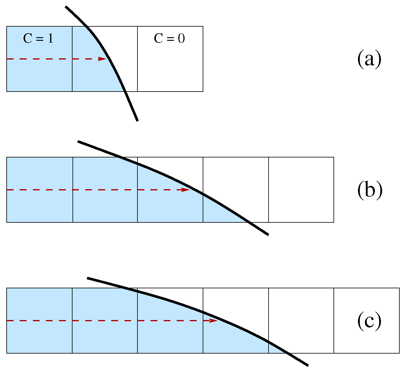
A way to consider this issue is to use the generalized height function (GHF) with an adaptive 1D stencil. In the present study, the maximum extension of the stencil is limited to 5 cells. In Figure 1, the height can be computed in the first two cases but not in the third one, where a stencil with at least 6 cells is required. However, in the last case, the height can probably be computed along the other coordinate direction. The HF value is stored as an offset from the center of the cell that contains it. An integer flag is set to indicate that the cell contains the HF and its orientation. A different value of the integer flag is used to indicate that a cell does not contain the HF value but that it was involved in the summation, as in the case of Figure 1b, where there are three cut cells, but only one contains the HF value. In isolated cut cells or with very complex local topologies, the midpoint of the Parker–Youngs reconstruction is considered [21]. Once the HF data have been computed, another sweep across the computational domain is required to collect triplets of HF values to compute and the local curvature and to interpolate these geometric properties of the interface in the cut cells where the HF is not present.
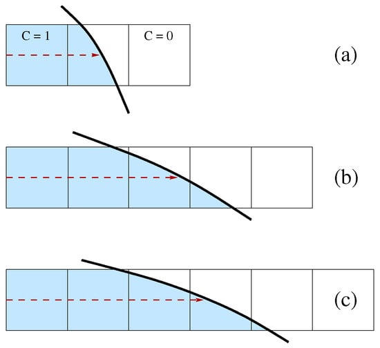
Figure 1.
One-dimensional adaptive stencil for height computation: (a) only three cells are required, (b) the whole stencil is necessary and (c) the stencil is not wide enough to compute the height.
2.2. Symmetry Considerations for the Machine Learning Model
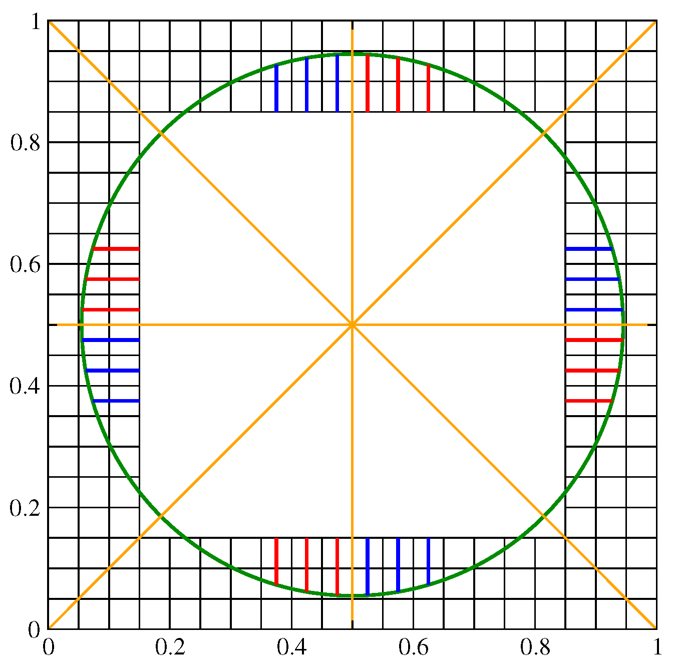
The curvature of an interface should be invariant under a few geometric transformations of the computational grid and the related volume fraction distribution. These transformations include reflections over a coordinate axis or the diagonal lines . A rotation of an angle that is a multiple of can be viewed as a sequence of such reflections. In Figure 2, a triplet of HF values of a given color, either red or blue, is clearly invariant with such a rotation. In particular, the symmetry axes are shown as yellow straight lines in that image. The set of red HF values is identical when considering a rotation of 90°. The same is true for the set of blue HF values. Furthermore, red HF values can be mapped onto the blue ones, and vice versa, with a reflection over the appropriate yellow line. The whole circumference can be reduced to an arc of 45° when considering all the rotations and reflections mentioned above.
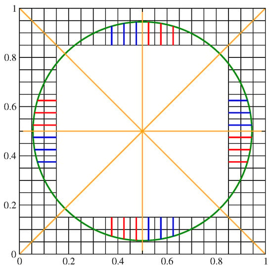
Figure 2.
Geometric sectors of a circular interface: each HF triplet of a given color, here either blue or red, can overlap with another one through a sequence of reflections over the symmetry axes (yellow straight lines).
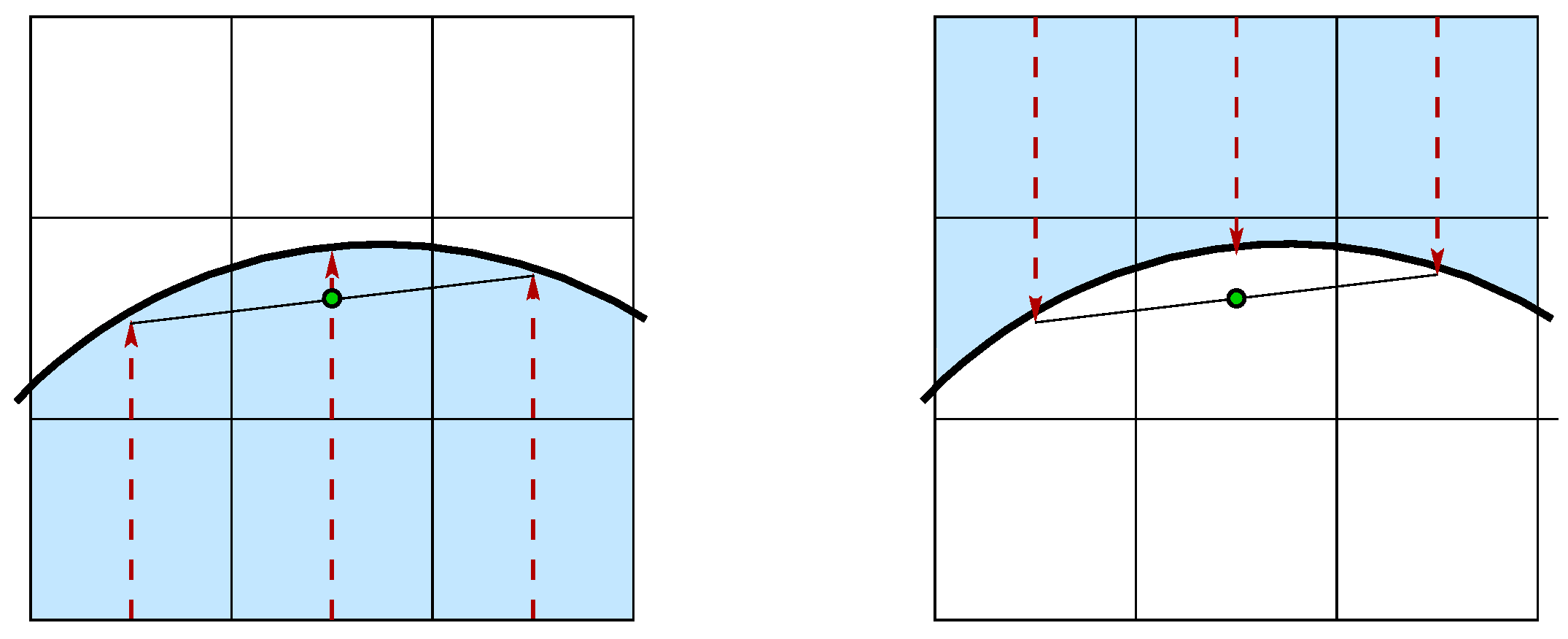
Independently from the sign convention, the curvature should change its sign when we swap the two fluid phases. As shown in Figure 3, when the interface is concave to the reference phase, the midpoint of the segment connecting the two side HF points is inside the phase with a height smaller than the central one; on the other hand, when the interface is convex, the midpoint is in the other phase, beyond the central HF point.
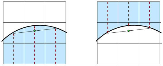
Figure 3.
The position of the midpoint connecting the two side HF points is inside the reference phase if the interface is concave (left), and it is outside if the interface is convex (right).
For this reason, only the first case is considered in the machine learning model since the curvature is always assumed to be positive, and then the two fluids are swapped when necessary.
Each HF point position is stored as an offset for the cell center. When the heights are collected to compute the geometric interface properties, these points are translated to the same local coordinate system. With three consecutive heights aligned along the same direction and the notation of Equations (8) and (9), the coordinates of the three HF points are , and . Lengths are then normalized to the grid spacing h with the origin of the local coordinate system placed on top of the central HF. The updated values of the coordinates of the three points are finally , and , with and . It is clear that the geometry of the HF triplet is fully described by the two independent parameters and . At low resolutions or with very complex topologies, it will be necessary to consider both vertical and horizontal height functions or even the midpoint of the Parker–Youngs reconstruction. In that case, the points coordinate after normalization are , and , and the number of independent parameters increases to 4.
The machine learning database is constructed only with geometries with a positive curvature value. The point with the highest HF value is always positioned to the left of the central value to preserve the invariance of the curvature to geometric transformations, .
3. Neural Network Model
This section describes the machine learning (ML) model used to calculate interface curvatures. The input data can be either the values of the color or the height function since the model is the same for all the different training datasets. Considering both the color function and the height function data, we analyze a huge set of input data and the performance of the ML model. We describe in detail both the methodology adopted for the training dataset and the structure of the neural network. The results are then compared to those obtained directly with the height function method to evaluate its accuracy and performance.
3.1. Data Generation
The quality of the training dataset strongly influences the performance of the machine learning model, so it is fundamental to generate a set that covers the whole range of input data that are expected to be found in actual two-phase flow simulations as close as possible. To this aim, a large number of circles are generated on a fixed Cartesian grid, each of them characterized by a random position of the center, , a random value of the radius, R, and of the angle, to determine a random point on the circumference. This ensures that the position of the interface is arbitrary without any alignment bias. Traditional methods for Direct Numerical Simulations (DNS) of two-phase flows perform accurately for a radius-to-grid ratio above 10. However, their performance degrades rapidly as that ratio decreases. Hence, we set the admissible radius range between and , where is the fixed grid spacing of the unit square. The radius distribution between these two limiting values can be determined with different approaches. A simple approach is to use a uniform distribution in the radius R, while a more target-oriented approach is to use a uniform distribution in the curvature , which results in a larger density of small radii when it is compared to the region of large radii. The uniform-in-curvature distribution guarantees that the training set spans all the output values we want to reproduce with similar density. On the other hand, in the uniform-in-radius approach, the density of training data with a large radius is comparatively much higher, so it can have unique orientations between the grid and the interface. Nevertheless, we have selected the uniform-in-curvature approach because, as already stated, traditional curvature reconstruction methods generally perform better at smaller curvature values and need a smaller density of training data in that range to achieve a good performance.
The generation of the training data can be summarized in the following procedure and is also represented in Algorithm 1. We start by setting seeds for the random number generator to ensure the reproducibility of the sequence of random numbers: we used the standard pseudo-random number generation routine available in the GNU libc library version 2.31, which is available in many Linux distributions. The quality of this distribution is somewhat limited but still adequate to generate the training data for machine learning [22]. We generate sets of random values , , by assuming that all they lay in the interval , or we can convert them to this interval when the generated numbers are integers in a given range. We set the curvature value as and determine the radius . We set the center to , with and , and the angle to to determine the point P on the circumference. We then locate the reference cell that contains P and consider a square section of the grid around that cell. Finally, we compute the volume fractions in that square section. The central block of volume fraction values is stored in a dataset. HF values around the reference cell are also computed, and the three HF central values are stored in another dataset.
| Algorithm 1 Generation of the training data |
|
The volume fraction field is initialized in each square cell of the computational grid with the new version of the Vofi library [23], which requires a user-defined implicit equation of the interface. This version optimizes and introduces a few new features with respect to the first release of the library [24].
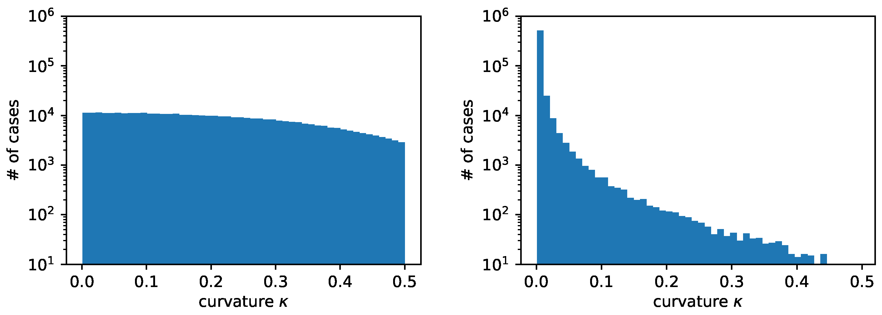
Figure 4 shows the distribution of radii with the two different approaches that we have previously described. We have considered random circles. The total number of cases obtained with the two distributions is quite different. In particular, we have generated cases with the uniform-in-curvature approach and cases with the uniform-in-radius approach. As previously stated, with the uniform-in-curvature approach, we have many more cases with circles having a small radius, where often it is not even possible to find three consecutive heights along the same direction, . On the contrary, with the uniform-in-radius approach, we have many more cases with a large radius, where the three consecutive heights are found along both coordinate directions, .

Figure 4.
Comparison of curvature distribution in the training dataset when using uniform curvature distribution (left) or uniform radius distribution (right) from the same random circles.
3.2. Treatment of Regular and Non-Regular Cases
As previously stated, when it is possible to find three consecutive HF values along the same coordinate direction and around the central cut cell that contains the discrete height , the number of independent parameters, which constitute the input data to train the neural network, is reduced to only two values, and . This standard case is called a regular one.
Figure 5 shows the distribution of the training dataset as a function of these two values and . The map on the left is obtained by using the uniform-in-curvature approach, while the one on the right considers the uniform-in-radius approach. It is clear that the second method heavily concentrates the values near the diagonal line where the curvature is smaller and dilutes them away from that line where the curvature is higher. On the contrary, the first approach provides a more uniform distribution of the pairs of values (, ).

Figure 5.
Comparison of scatter plot maps of the training dataset when using uniform curvature distribution (left) or uniform radius distribution (right) from the same random circles.
The heights can be computed along the two coordinate directions x and y. When the two computations are possible, that is to say, three consecutive HF values are found along both coordinate directions, we add the two sets to the dataset.
In this study, a slightly different neural network has been trained with a second dataset that contains the non-regular cases. These cases occur when three consecutive height points do not exist along the same coordinate direction. To be able to extend the methodology to very high curvatures, we have devised a methodology that combines the vertical and horizontal heights that are available in the block of cells centered around the cut cell that contains the height . When the total number of vertical and horizontal heights is equal to three, the coordinates of these three HF points can be written as , and , with 4 independent parameters.
However, a relatively common situation is where we can find two heights in both directions. In that case, the best solution is to consider two heights from one direction and select the third one in the other direction to enlarge the footprint of the selected set as much as possible. Failure to do so may lead to two HF points on the interface that are excessively close to each other with a possible inaccurate curvature estimate. In general, the non-regular case leads to a non-uniform distribution of HF values and forces the neural network to handle a wider range of scenarios. However, as the standard height function method needs to be changed or integrated with another method at low resolution, we do not present that scenario in this paper, where we study only the high-resolution or asymptotic region.
3.3. Neural Network Definition and Training
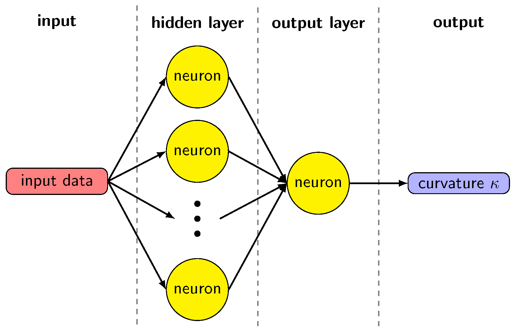
The machine learning model for the curvature evaluation is based on a two-layer feed-forward neural network with N neurons in the hidden layer and a single neuron in the output layer, as shown in Figure 6. This structure of the network is effective when mapping a continuous set onto another [25], which is the one we obtain starting from the set of volume fractions or height functions, and compute a curvature value. A single output value justifies a single neuron in the output layer. The neurons in the hidden layer have an activation function based on the hyperbolic tangent, given the non-linear relation between volume fractions or height functions and the curvature. We have tested the network with a different number of neurons in the hidden layers, with 25, 50, 75, 100, 125. Figure 7 shows the behavior of the mean square error as a function of . The MSE decreases significantly for the lowest values of , but it saturates when is greater than 75. With a smaller number of neurons, the network cannot suitably reproduce the sets of values in the dataset. On the other hand, using a large set does not give any appreciable gain, while significantly extending the computational time required to train the model. Therefore, we choose the value to compare the results with the literature [19].
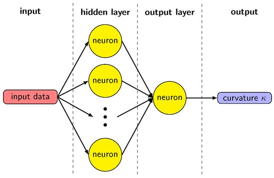
Figure 6.
Diagram of the neural network.
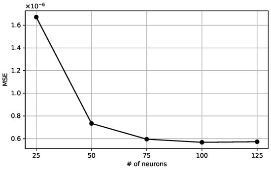
Figure 7.
Mean Square Error as a function of the number of neurons in the hidden layer. The range is scaled down by a factor of .
The input dataset is a -by-2 or -by-9 matrix, where is the number of entries. Each entry is made up of the 2 parameters and in the first matrix, or the 9 values of the volume fraction around the central cell in the other one. In the following, will represent the value 2 or 9 based on the training dataset under consideration, when no ambiguity is present. A dataset with exact curvature values is also considered and we will refer to each single value as the target . The output y of the neural network can be written as
where are the weights associated to the k-th neuron in the hidden layer and j-th input value, and is the bias of the k-th neuron. The output layer neuron is marked by the superscript 0. The values of and are computed during the training. We can then introduce the mean square error (MSE), defined as
This quantity measures the distance between the neural network solutions and the exact values . In a typical machine learning framework, the input dataset is split into a training set, a validation set, and a testing set, with weights of 70%, 15%, and 15%, respectively. The weights and biases are adjusted to minimize the MSE of the training dataset only. The neural network is implemented in the MATLAB version 2023.1 deep learning toolbox [25], with the Levenberg–Marquardt algorithm [26,27] used to minimize the MSE. The input dataset passes many times through the neural network, each pass is referred to as an epoch, and the MSE for the training, validation, and testing sets is constantly monitored. The process is stopped after 6 consecutive iterations in which the MSE does not change appreciably, according to a given tolerance, or the number of epochs reaches the threshold of 1000. For all the results shown later in the text, the convergence of the procedure is reached before the threshold, typically around 700–800 epochs.
Other backpropagation algorithms are available in the deep learning toolbox. Their performance was always inferior to the Levenberg–Marquardt neural network model. Once the neural network has been run, all the weights and biases are stored and used without any further access to the input dataset.
4. Results
The neural network approach is applied to an extensive input dataset of height function values and the obtained results are presented in this section. We consider randomly generated points on circular interfaces with a different radius, and a Cartesian uniform grid with spacing h in the unit square. To create a complete dataset distributed evenly within the target limits, we choose a random and uniform distribution of curvatures ranging from to , corresponding to and . The input and output datasets, generated by this distribution, contain entries. The input dataset is organized as an array of HF differences, and , and the output dataset as a array of the corresponding curvature values, acting as the targets for our analysis. We remark that the total number of entries does not equal the number of randomly generated cases because the input dataset ignores the cases where less than 3 heights are found in the block of cells.
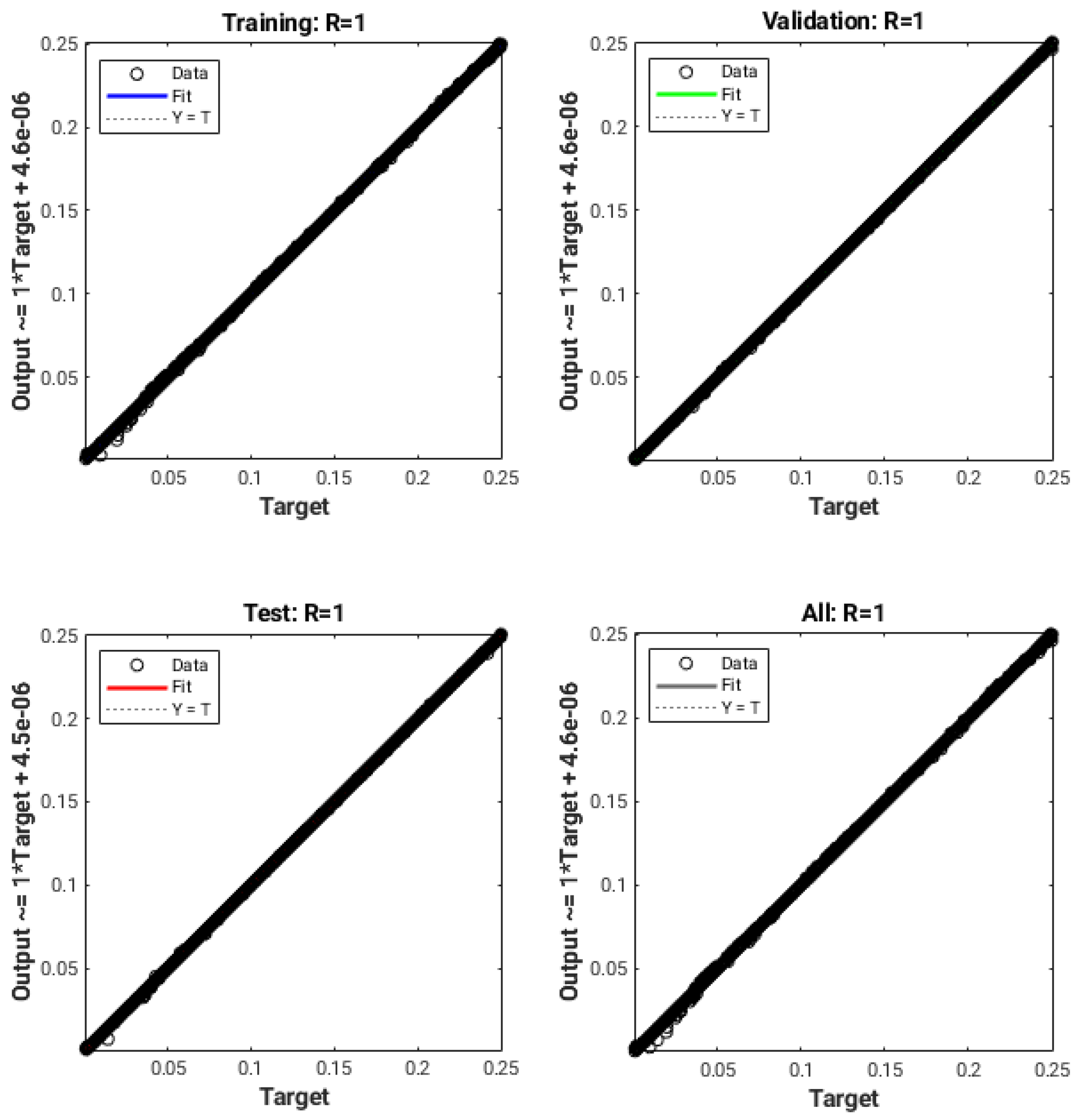
The data fitting was performed using Matlab with its built-in Neural Network Toolbox, as previously described. The training process ends when the MSE value of Equation (12) does not improve for 6 consecutive epochs or the total epoch count reaches 1000. Figure 8 shows the results obtained with the uniform-in-curvature training dataset. The evaluation involves the comparison of the output, which consists of the curvatures predicted by the neural network, with the target values representing the exact curvatures. For each data subset (training, validation, and testing) and for the entire dataset, a regression line and the correlation coefficient R have been calculated. It can be noticed in Figure 8, that the coefficient R is basically equal to 1, and therefore, the theoretical lines (in color in the various graphs) are completely covered by the dataset points. The error in absolute value between the numerical curvatures and the corresponding target values is always less than for all the entries in the dataset. This indicates a very good accuracy and a successful fit between the computed and the actual values of the curvature.
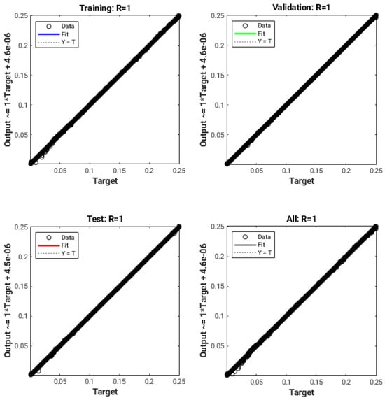
Figure 8.
Scatter plots of predicted and target values for the training, validation, testing, and complete data sets, using the uniform distribution in curvature. The coordinate axes span the range of curvatures between 0.0 and 0.25.
We have also considered the corresponding input dataset organized as a array of volume fraction data. With this more homogeneous dataset, we observe an increase in the value of the overall correlation coefficient from R of [19], where only a limited number of circular interfaces were considered, to R .
4.1. Circle Test Case
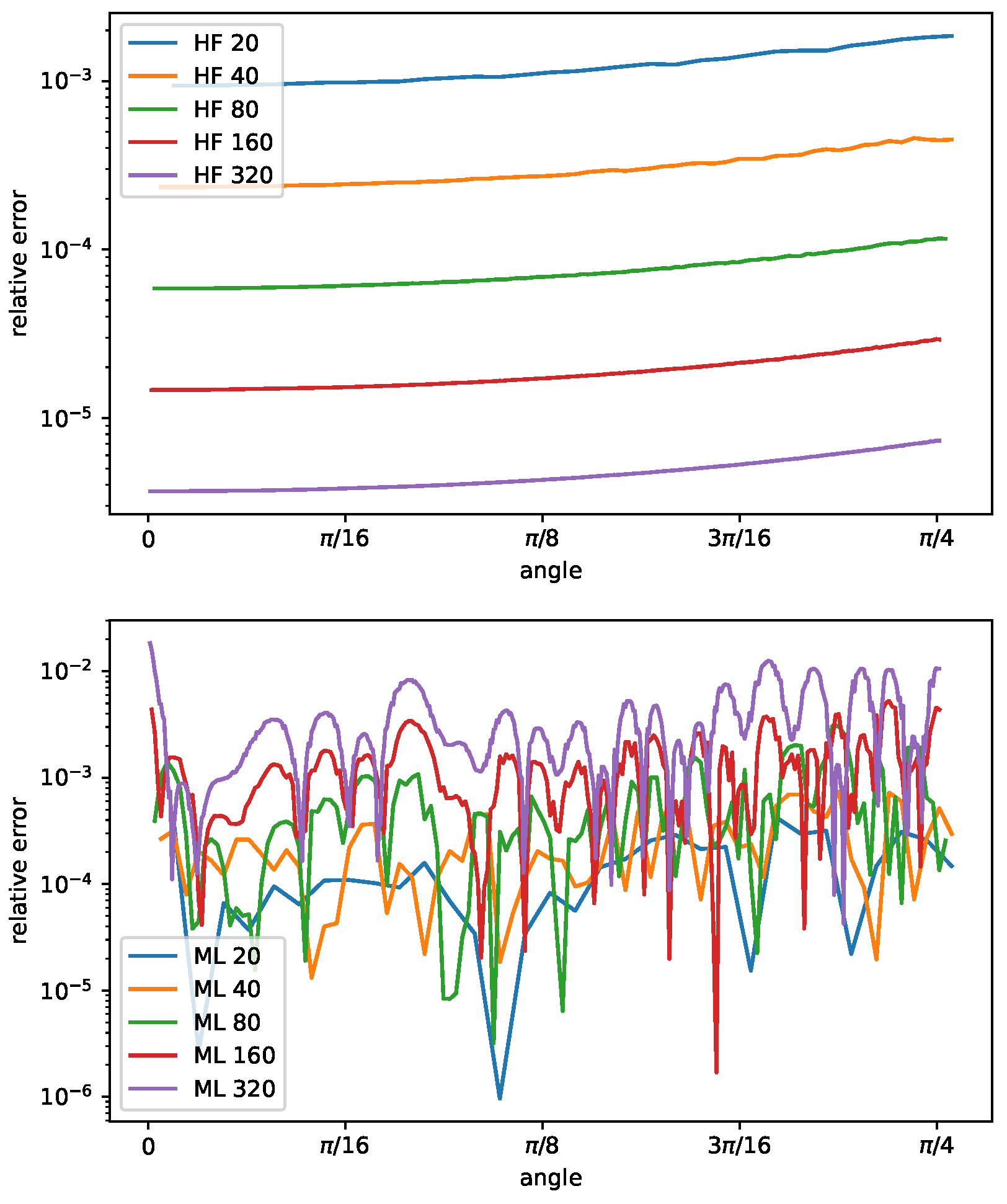
In Figure 9, we show the relative error of the curvature as a function of the angle , for different radii R, ranging from to , computed with the height function method and the machine learning approach. The circles that have been considered are not present in the input database. The relative error scales quadratically with the radius R, or equivalently by increasing the grid resolution, for the HF method. Furthermore, the error increases from , where the interface is almost aligned with the computational grid, to , where the interface cuts the grid diagonally. These results are consistent with the theory detailed in [8]. The bottom part of Figure 9 reports the same graph obtained with the machine learning approach. In this case, the relative error does not scale with the grid resolution and does not show any clear behavior with the angle variation. The machine learning approach shows no convergence when the curvature decreases, leading to a graph with superimposed lines with similar errors independent of angle and curvature.

Figure 9.
Curvature relative error as a function of the angle , , for circles with ratio equal to , for the height function method (top) and the machine learning model (bottom).
To compare the convergence of the different approaches, we consider the and error norms, as defined in [9]:
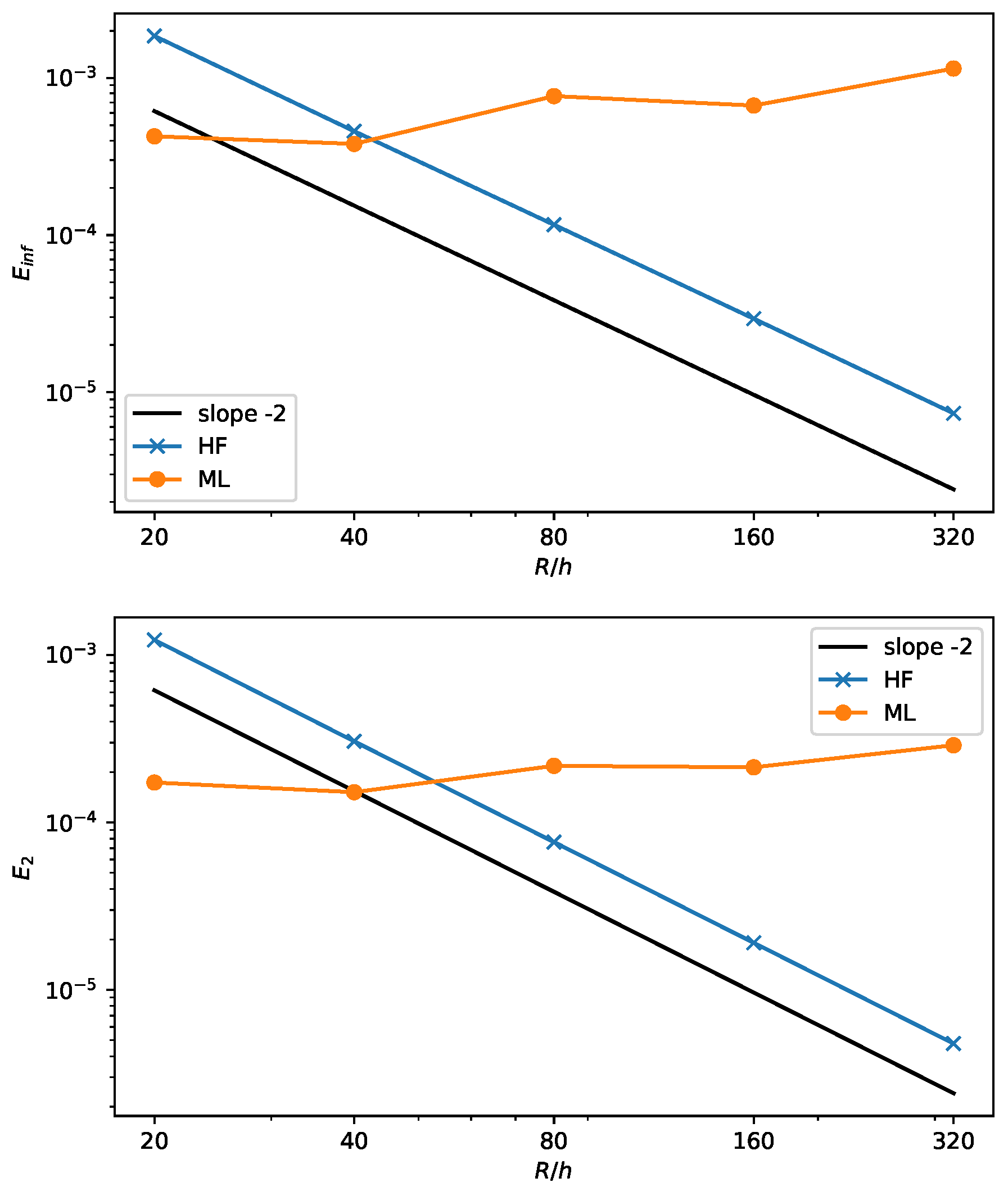
where is the numerical value and the reference curvature. The results are shown in Figure 10 for a circle with a fixed radius and variable grid spacing h. The line with a constant slope equal to is also depicted.
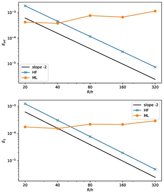
Figure 10.
Infinite error (top) and mean squared error (bottom) for the ML and HF methods with increasing circle resolution.
As expected, the height function method scales quadratically, as demonstrated in [8]. On the other hand, the machine learning results reflect the lack of convergence, see also Figure 9, with an almost flat value of the error that does not change with h. Nevertheless, the error is rather small. A similar behavior is also found in [9,20] for different geometrical configurations of the interface.
4.2. Four-Petaled Star Test Case
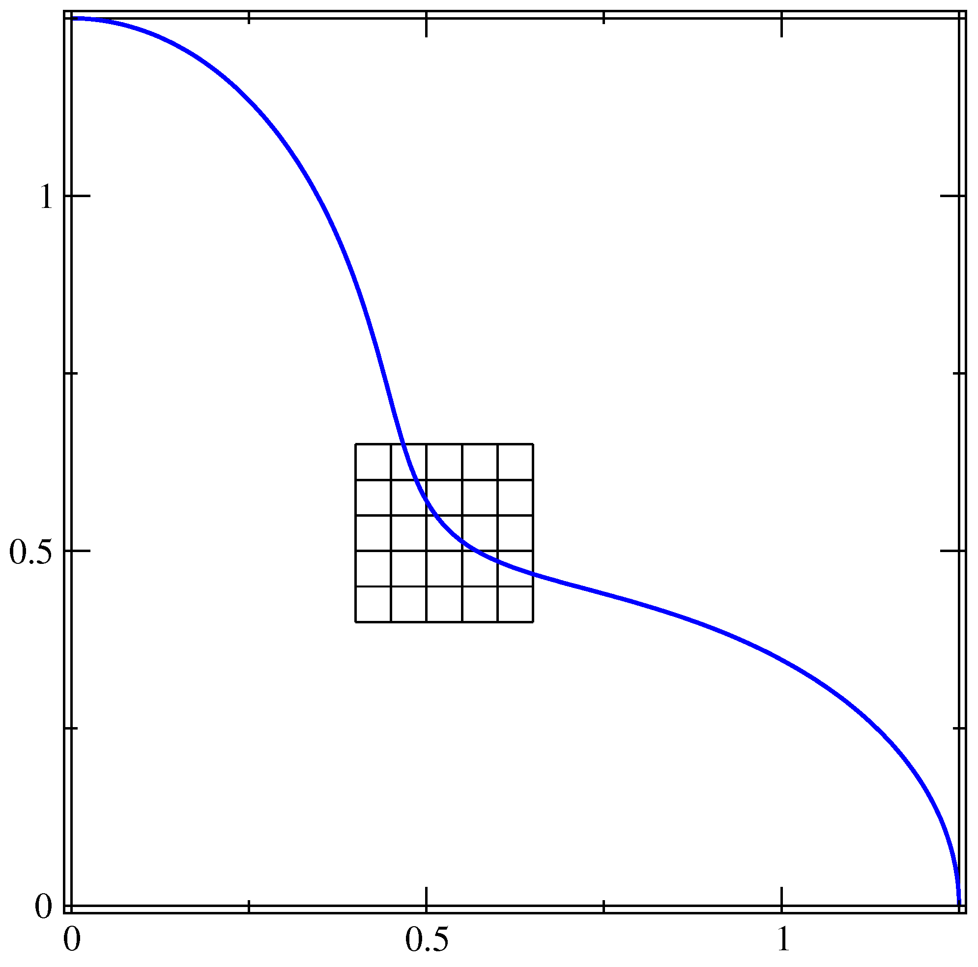
An additional test has been performed on a more complex interface with variable curvature. The test is based on the four-petaled star introduced in [9]. The parametric equations of the interface line as a function of the angle are
where is the base radius, is the amplitude of the oscillation and is the number of petals. In this test, is equal to 1, is equal to 0.25 and . Given the symmetry of the interface, in Figure 11, we show the interface only in the upper-right quadrant together with a portion of the grid at the lowest resolution, . This setup has been chosen to compare our results with those obtained in [9]. In the angular range shown in Figure 11, the interface presents two points where the convexity changes and the curvature is zero, and regions where the curvature value is either positive or negative.

Figure 11.
Interface line of the four-petaled star in the upper-right quadrant. The full line can be obtained with two consecutive reflections over the coordinate axes. A small portion of the grid at the lowest resolution is also shown.
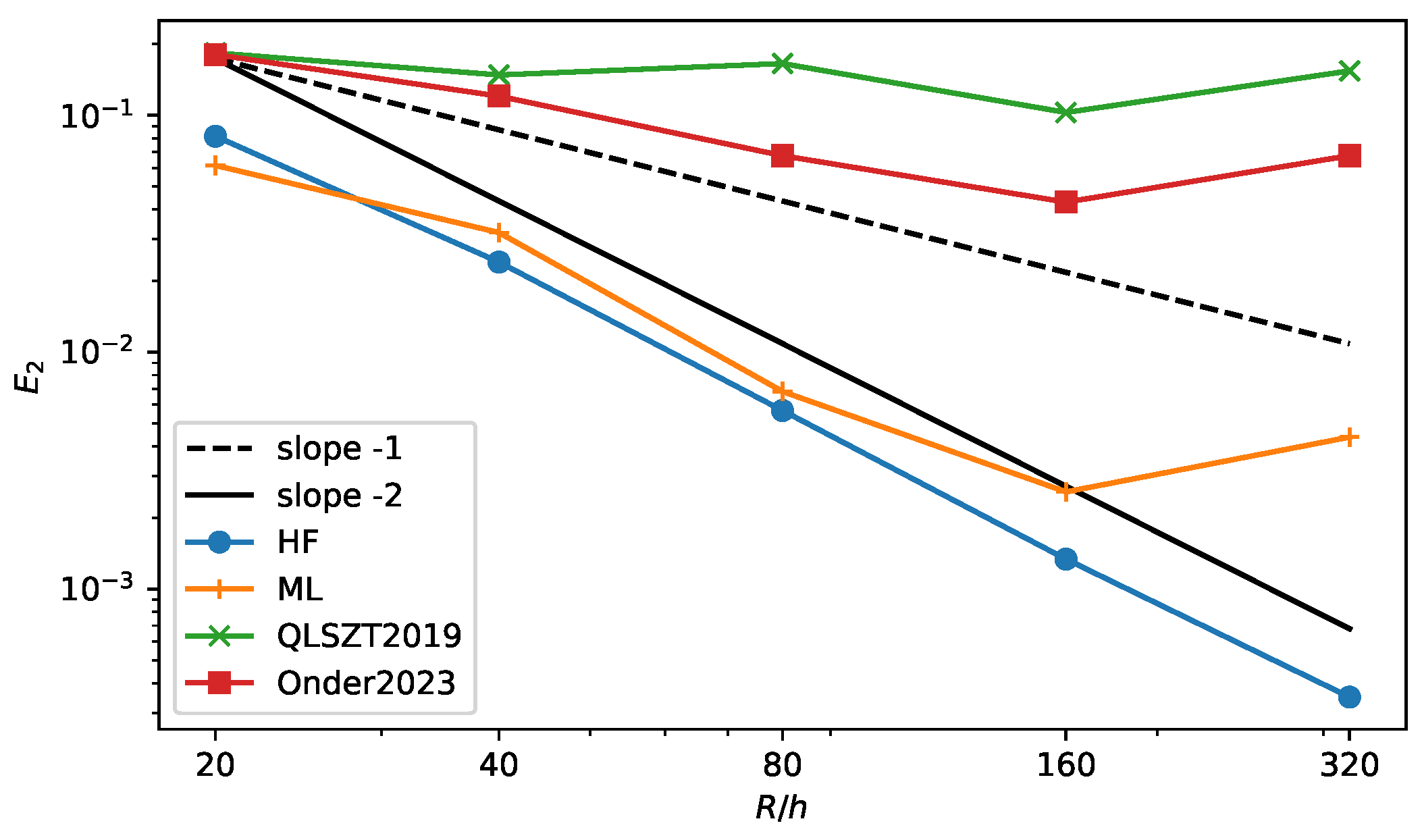
The error in the curvature calculation is shown in Figure 12 for the HF method (HF line) and a few machine learning methods—in particular, the method presented in this paper (ML line), the method from [19] (QLSTZ2019 line) and the SymMLP method from [9] (Onder2023 line). The new algorithm shows a lower value of the error at all resolutions when compared to the other two ML approaches. Furthermore, the error scales similarly to the HF method, but again, it stops converging at the highest resolution. It is interesting to see that at the lowest resolution, it performs better the the HF method, as was the case for the circle test. This is an interesting feature because the HF method degrades for very coarse resolutions when it is not possible to construct three proper height values around a cut cell. We can then think of a hybrid method that relies on the HF method at intermediate and high resolutions and that switches to the ML method at low resolutions. A similar method has been implemented in [14] that uses the convolution method at low resolution. We plan to explore this strategy in future works.
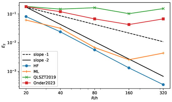
Figure 12.
error for the four-petaled star interface as a function of the grid resolution. Comparison of the Height Function method (HF), the Machine Learning method from this article (ML), the original ML method from [19] (QLSZT2019) and the SymMLP from [9] (Onder2023).
5. Conclusions
In this work, we have explored an alternative approach for computing curvature in two-phase flow simulations with the Volume of Fluid (VOF) method by employing machine learning techniques. We have used the height function data in combination with machine learning to develop a neural network model capable of efficiently predicting the local interface curvature. Since the fluid forces can easily predominate over the capillary one, in this paper, we have tested the accuracy of the curvature computation without motion and leave dynamic tests for future papers. The proposed model is tested on different geometric shapes and compared with the HF method based on the same volume fractions. The state-of-the-art HF method has been widely used to compute curvature on smooth and low-varying interfaces. However, we note it may face accuracy loss in non-regular cases where three consecutive height points do not exist in any direction. To overcome this limitation, a novel neural network model has been developed by training it with the HF data. Our approach aims to handle regular and non-regular cases by creating a synthetic dataset with a wide range of interface curvatures. When an optimal alignment between the predicted curvatures and the exact curvatures can be found, the neural network achieves a high degree of accuracy. However, it is worth noting that while the HF method scales quadratically with the grid resolution, the machine learning prediction does not.
The computational cost associated with the height function method is typically only a fraction of that associated with a two-phase flow solver, so, in general, the time reduction that the machine learning algorithm would provide does not justify, at this stage, the loss in accuracy with resolution. A case can be made for the ML approach in situations where the HF method is not robust or accurate enough, i.e., when the radius of the bubble or droplet is close to the mesh spacing. Further analysis should be carried out in this direction, as well as in the improvement of the ML methodology.
Author Contributions
Conceptualization, A.C. and R.S.; methodology, A.C., R.S. and L.S.; software, A.C., R.S. and L.S.; validation, A.C., R.S. and L.S.; formal analysis, A.C., S.M., R.S. and L.S.; investigation, A.C., S.M., R.S. and L.S.; writing—original draft preparation, A.C., S.M., R.S. and L.S.; writing—review and editing, A.C., S.M., R.S. and L.S. All authors have read and agreed to the published version of the manuscript.
Funding
This research received no external funding.
Data Availability Statement
The original contributions presented in the study are included in the article, further inquiries can be directed to the corresponding author.
Conflicts of Interest
The authors declare no conflicts of interest.
References
- Tryggvason, G.; Scardovelli, R.; Zaleski, S. Direct Numerical Simulations of Gas–Liquid Multiphase Flows; Cambridge University Press: Cambridge, UK, 2011. [Google Scholar]
- Chirco, L.; Da Vià, R.; Manservisi, S. VOF evaluation of the surface tension by using variational representation and Galerkin interpolation projection. J. Comput. Phys. 2019, 395, 537–562. [Google Scholar] [CrossRef]
- Cummins, S.J.; Francois, M.M.; Kothe, D.B. Estimating curvature from volume fractions. Comput. Struct. 2005, 83, 425–434. [Google Scholar] [CrossRef]
- Brackbill, J.U.; Kothe, D.B.; Zemach, C. A continuum method for modeling surface tension. J. Comput. Phys. 1992, 100, 335–354. [Google Scholar] [CrossRef]
- Cerroni, D.; Da Vià, R.; Manservisi, S. A projection method for coupling two-phase VOF and fluid structure interaction simulations. J. Comput. Phys. 2018, 354, 646–671. [Google Scholar] [CrossRef]
- Hirt, C.W.; Nichols, B.D. Volume of Fluid (VOF) Method for the Dynamics of Free Boundaries. J. Comput. Phys. 1981, 39, 201–225. [Google Scholar] [CrossRef]
- Buhendwa, A.B.; Bezgin, D.A.; Adams, N.A. Consistent and symmetry preserving data-driven interface reconstruction for the level-set method. J. Comput. Phys. 2022, 457, 111049. [Google Scholar] [CrossRef]
- Bornia, G.; Cervone, A.; Manservisi, S.; Scardovelli, R.; Zaleski, S. On the properties and limitations of the height function method in two–dimensional Cartesian geometry. J. Comput. Phys. 2011, 230, 851–862. [Google Scholar] [CrossRef]
- Önder, A.; Liu, P.L.F. Deep learning of interfacial curvature: A symmetry-preserving approach for the volume of fluid method. J. Comput. Phys. 2023, 485, 112110. [Google Scholar] [CrossRef]
- Ataei, M.; Bussmann, M.; Shaayegan, V.; Costa, F.; Han, S.; Park, C.B. NPLIC: A machine learning approach to piecewise linear interface construction. Comput. Fluids 2021, 223, 104950. [Google Scholar] [CrossRef]
- Han, A.; Evrard, F.; Desjardins, O. Comparison of methods for curvature estimation from volume fractions. Int. J. Multiph. Flow 2024, 174, 104769. [Google Scholar] [CrossRef]
- Owkes, M.; Desjardins, O. A mesh-decoupled height function method for computing interface curvature. J. Comput. Phys. 2015, 281, 285–300. [Google Scholar] [CrossRef]
- Popinet, S. An accurate adaptive solver for surface–tension–driven interfacial flows. J. Comput. Phys. 2009, 228, 5838–5866. [Google Scholar] [CrossRef]
- Patel, H.V.; Kuipers, J.A.; Peters, E.A. Computing interface curvature from volume fractions: A hybrid approach. Comput. Fluids 2018, 161, 74–88. [Google Scholar] [CrossRef]
- Svyetlichnyy, D. Neural networks for determining the vector normal to the surface in CFD, LBM and CA applications. Int. J. Numer. Methods Heat Fluid Flow 2018, 28, 1754–1773. [Google Scholar] [CrossRef]
- Kumar, B.; Singh, N.K. Curvature Estimation in Context of Interface Capturing Using Machine Learning. In Proceedings of the 9th Thermal and Fluids Engineering Conference (TFEC), Corvallis, OR, USA, 21–24 April 2024. [Google Scholar]
- Haghshenas, M.; Kumar, R. Curvature estimation modeling using machine learning for CLSVOF method: Comparison with conventional methods. In Proceedings of the Fluids Engineering Division Summer Meeting, San Francisco, CA, USA, 28 July–1 August 2019; American Society of Mechanical Engineers: New York, NY, USA, 2019; Volume 59032, p. V002T02A078. [Google Scholar]
- Kumar, B.; Chand, S.; Singh, N.K. Local interface remapping based curvature computation on unstructured grids in volume of fluid methods using machine learning. Phys. Fluids 2024, 36, 062107. [Google Scholar] [CrossRef]
- Qi, Y.; Lu, J.; Scardovelli, R.; Zaleski, S.; Tryggvason, G. Computing curvature for volume of fluid methods using machine learning. J. Comput. Phys. 2019, 377, 155–161. [Google Scholar] [CrossRef]
- Patel, H.V.; Panda, A.; Kuipers, J.A.M.; Peters, E.A.J.F. Computing interface curvature from volume fractions: A machine learning approach. Comput. Fluids 2019, 193, 104263. [Google Scholar] [CrossRef]
- Parker, B.J.; Youngs, D.L. Two and Three Dimensional Eulerian Simulation of Fluid Flow with Material Interfaces; Technical Report 01/92; UK Atomic Weapons Establishment: Berkshire, UK, 1992. [Google Scholar]
- Shacham, H.; Page, M.; Pfaff, B.; Goh, E.J.; Modadugu, N.; Boneh, D. On the effectiveness of address-space randomization. In Proceedings of the 11th ACM Conference On Computer and Communications Security, Washington, DC, USA, 25–29 October 2004; pp. 298–307. [Google Scholar]
- Chierici, A.; Chirco, L.; Chenadec, V.L.; Scardovelli, R.; Yecko, P.; Zaleski, S. An optimized VOFI library to initialize the volume fraction field. Comput. Phys. Commun. 2022, 281, 108506. [Google Scholar] [CrossRef]
- Bnà, S.; Manservisi, S.; Scardovelli, R.; Yecko, P.; Zaleski, S. Vofi—A library to initialize the volume fraction scalar field. Comput. Phys. Commun. 2016, 200, 291–299. [Google Scholar] [CrossRef]
- Beale, M.H.; Hagan, M.T.; Demuth, H.B. Neural network toolbox. In User’s Guide; MathWorks: Natick, MA, USA, 2010; Volume 2, pp. 77–81. [Google Scholar]
- Roweis, S. Levenberg-Marquardt Optimization; Notes; University Of Toronto: Toronto, ON, Canada, 1996; Volume 52. [Google Scholar]
- Yan, Z.; Zhong, S.; Lin, L.; Cui, Z. Adaptive Levenberg–Marquardt algorithm: A new optimization strategy for Levenberg–Marquardt neural networks. Mathematics 2021, 9, 2176. [Google Scholar] [CrossRef]
Disclaimer/Publisher’s Note: The statements, opinions and data contained in all publications are solely those of the individual author(s) and contributor(s) and not of MDPI and/or the editor(s). MDPI and/or the editor(s) disclaim responsibility for any injury to people or property resulting from any ideas, methods, instructions or products referred to in the content. |
© 2024 by the authors. Licensee MDPI, Basel, Switzerland. This article is an open access article distributed under the terms and conditions of the Creative Commons Attribution (CC BY) license (https://creativecommons.org/licenses/by/4.0/).

