Abstract
Hydraulic turbines have become indispensable for harnessing renewable energy sources, particularly in-pipe hydraulic turbine technology, which leverages excess energy within pipeline systems like drinking water distribution pipes to produce electrical power. Among these turbines, the propeller-type axial turbine with circular blades stands out for its efficiency. However, there is a notable lack of literature on fluid dynamics and structural behavior under various operational conditions. This study introduces a comprehensive methodology to numerically investigate the hydraulic and structural responses of turbines designed for in-pipe installation. The methodology encompasses the design of circular blades, followed by parametric studies on fluid dynamics and structural analysis. The circular blade’s performance was evaluated across different materials, incorporating static, modal, and harmonic response analyses. Results showed that the circular blade achieved a peak hydraulic efficiency of 75.5% at a flow rate of 10 l/s, generating 1.86 m of head pressure drop and 138 W of mechanical power. Structurally, it demonstrated a safety factor exceeding 1 across the entire hydraulic range without encountering resonance or fatigue issues. This research and its methodology significantly contribute to advancing the understanding of designing and assessing the fluid dynamic behavior and structural integrity of circular blades in axial propeller-type turbines for in-pipe installations, serving as a valuable resource for future studies in similar domains.
1. Introduction
In recent years, concerns about the environment, economy, and resource sustainability have driven a growing focus on energy efficiency. This shift is significant in turbines, essential for tapping into renewable energy sources. Efficient energy systems are vital for lessening harm and improving the economic viability of power production. Hydraulic turbines play a role in enhancing energy recovery and system efficiency. The effectiveness of these turbines directly affects the expenses and eco-friendliness of power plants [1]. In energy production processes through turbines inside pipelines such as Savonius, Michell–Banki, and spherical Darrieus turbines develop an efficiency of 40% [2,3,4]. In comparison, PAT (Pump as Turbine) technology presents up to 70% efficiencies [5], and the propeller type reaches up to 76% [6].
Maintaining pressure levels in water distribution systems is critical and often regulated by industry standards [7,8]. Conventional pressure-regulating valves commonly waste energy as heat, resulting in energy loss. However, integrating turbines into these systems has shown promise in capturing and utilizing this excess materialized energy to enhance system efficiency. For instance, Hannachi et al. designed a new pressure control mechanism that incorporates a Banki turbine with an integrated flap adjustment device, achieving efficiencies of up to 76% in recovering energy from water networks [9]. Finally, the study of Pasha et al. [10] showed that the greater the number of storage tanks, the more uniform the pressure distribution across the piping system, which in turn allows excess potential energy to be stored and then converted in the turbines into mechanical and electrical energy.
In terms of the in-pipe turbine’s optimal functionality, the fluid exerts a hydraulic load on the blades due to its velocity. This force causes the blades to rotate, which is then transferred to the shaft connected to a generator. As the shaft rotates, it spins the generator, converting the mechanical energy into electrical energy. However, the mechanical drive torque may induce abnormal stresses and deformations that provoke structural failure of some turbine components [11]. These failures are often due to hydrodynamic, inertial, centrifugal, and gravitational forces that produce significant vibrations and deformations over the blades [12]. As a result, a deep analysis of the hydrodynamic and structural performance of the turbine’s components becomes vital to improve the design and costs of in-pipe hydraulic turbines [11].
In previous studies, it is possible to find fluid–structure analyses to determine the blade failure probability and evaluate the blade stress [13,14,15]. Other approaches consider the incidence of the materials with their respective roughness on the global performance of the turbine [16,17,18]. For example, they found that the turbine weight is a crucial element in the stress suffered by the machine shaft and how system leakage causes premature equipment wear due to the erosion phenomenon [19]. Also, they stressed the importance of refining these designs using Box Behnken Design and NSGA II algorithms to optimize energy efficiency and how turbine structure and operation enhancements contribute to improved efficiency curves and operational adaptability, which are essential for use and long-term performance [1]. In addition to structural-based studies, dynamic analyses serve to obtain higher reliability levels of the structural response of this type of turbomachinery. Xia et al. [20] found that the fundamental vibrations modes of simplified cantilever blade structures (i.e., no shaft) are primarily shaped by the vibrations of the blades, which are organized into mode families. Each family’s characteristics strictly depend on the number of blades, showing a clear pattern in frequency bands. The modal vibration of the turbine’s shaft and blades tends to couple. This coupling can lead to abnormal shifts in some modal families’ behaviors, scattering the natural frequencies and increasing the likelihood of resonance. They also found that the bearing stiffness close to the runner and the blade opening affects mode coupling and the frequency bandwidths. It was observed that increased bearing stiffness results in narrower frequency bandwidths, suggesting a potential approach to controlling vibrational characteristics. Likewise, An et al. [21] studied the same scenario, and they found that the bearing stiffness predominantly manifested as vibrations on the blades. These vibrations can be classified into mode families based on the single-blade modes, which correspond to a series of frequency bands with very small widths. They also found that understanding these modal characteristics can help predict and mitigate resonance in turbine designs, thereby improving axial turbines’ operational stability and efficiency to better simulate real-world performance challenges. Linet al. [22] successfully validated the finite element model (FEM) used for predicting the dynamic behavior and strength characteristics of turbine rotors under operational conditions. Their work demonstrated that the mode shapes and natural frequencies derived from the FEM correlate well with those obtained from experimental modal analysis (EMA), using the Modal Assurance Criterion (MAC) for verification. Additionally, the study highlights that the stress distribution across the rotor, caused by centrifugal and aerodynamic forces during operation, can be accurately predicted using the FEM, thereby providing a reliable method for assessing rotor durability and structural integrity in real-world conditions. This type of study to estimate structural fatigue, the vibrational response to a realistic spectrum of excitations, and the associated equivalent damping has achieved differences between numerical and experimental results of less than 10% [23], which suggests it is a reliable methodology but needs exploration into more complex scenarios.
Some other studies focus on improving turbine blade performance through passive morphing using advanced computational FSI analysis. For instance, Castorrini et al. [24] employed sophisticated stabilization techniques to handle the turbulent flow dynamics, which is crucial for in-pipe systems where flow conditions can significantly impact turbine efficiency and blade stress. However, applying these findings to circular blade designs in axial propeller turbines still needs to be explored, highlighting a research opportunity. Previous studies [25] integrated fluid, thermal, and structural interaction modeling to predict the life of turbine blades under extreme operational conditions. This comprehensive approach is pertinent for designing in-pipe axial turbines with circular blades, where varying thermal and flow conditions can drastically affect lifespan and performance. However, specific challenges related to the unique environment of in-pipe systems, such as confined flows and the potential for increased turbulence, remain unexplored. Krishna et al. [26] incorporated two-way fluid–structure simulations to study a marine propeller, where two-way simulations allow for the prediction of the hydroelastic response of the propeller. For this purpose, they used the Large Eddy Simulation (LES) turbulence model and the Ffowcs Williams–Hawkings (FWH) acoustic model, which is used to evaluate the sound pressure level generated by the propeller (SPL). The main difference is that the two-way FSI can accommodate the maximum value of stress and strain developed during the initial part of the transient solution, which is essential in propeller design.
In this work, we focused on the propeller-type turbine with circular blades because it closely matches hydraulic efficiencies of around 76% without using passive elements such as guide vanes [27,28]. Thus, this research aims to improve the design of in-pipe turbines with circular blades to boost their durability and energy conversion efficiency by combining cutting-edge numerical models. The study seeks to uncover knowledge about how fluids interact with turbine blade structure, paving the way for greener and more effective renewable energy solutions.
The novelty of this paper consists in offering to the scientific literature an easily replicable and reproducible methodology for the fluid–structure analysis of propeller-type turbines not only considering the static mechanical analysis but also dynamical, which will facilitate the process for future research thanks to the computational tools developed and offered in a free form, making it possible for this work to contribute to engineering practices by pushing the limits of turbine technology and laying the groundwork for future advancements in renewable energy applications by:
- Providing the scientific literature with a methodology to analyze the hydrodynamic performance and structural (static, modal, and harmonic) behavior of an axial propeller-type turbine with circular blades for in-pipe installation in water distribution systems. Previous fluid–structure analyses reported in the scientific literature do not structurally study this type of turbine with a constant thickness curved blade, especially considering resonance and fatigue conditions for different materials which can be scaled to other types of turbomachines.
- Offering the scientific community a couple of open-source computational tools to perform the grid convergence study by applying the Grid Convergence Index method (GCI) recommended by The American Society of Mechanical Engineers (ASME) and provide the meridional coordinates of the circular blade to obtain its three-dimensional model.
This paper is divided into five sections. Section 1 describes the state of the art around the topic at hand, identifies the potential research opportunities, and states the main contribution of this work. Section 2 contains the design of a turbine blade with constant curvature and thickness known as a “circular blade”. Section 3 states the proposed methodology used to carry out the one-way fluid–structure interaction (FSI) parametric simulations applied to the circular blade. Section 4 reports the numerical model validation and compiles and analyzes the fluid dynamic and structural results. Finally, Section 5 concludes the findings of the work and states the plausible future works associated with the present research.
2. Circular Blade 3D Model
This section presents the design process of a circular blade for an axial propeller-type turbine. The goal is to obtain a three-dimensional blade model and its corresponding control volume to perform the fluid dynamic and structural simulations. First, the design parameters are selected based on previous studies (see Table 1) and a series of physical and capacity restrictions from a hydraulic test bench. Moreover, we show the theoretical design process of the circular blade and the assumptions made. Lastly, we report the blade geometry generation methodology using a coordinate transformation process, which results are fed into Ansys BladeGen.

Table 1.
Axial propeller-type turbine design parameters used in different studies.
2.1. Design Parameters Selection
Table 1 presents a compilation of the parameters used by different authors for designing axial propeller-type turbine blades. The turbine design’s initial parameters are the flow rate Q, the available head pressure H, the assumed hydraulic efficiency , the angular velocity N, the mechanical power , the outer diameter , the ratio between the inner and outer diameters , and the number of blades z. According to this information, we identified that the propeller-type turbines have a wide application margin concerning the working conditions they can operate at due to the wide range of the values’ variation. Therefore, the design parameters could range for each design parameter as follows: l/s, m, %, rpm, W, mm, , .
Table 2 reports the design parameters used to generate the circular blade proposed in this work. The table specifies the turbine and piping sizing parameters and the assumed hydraulic design parameters. First, we determined the pipe’s internal diameter based on a commercial 3-inch PVC pipe with Schedule 40. A blade clearance of mm was assumed to maximize the turbine efficiency, as demonstrated by the research of Tran et al. [45]. Once was defined, we determined the turbine’s outer diameter. The turbine’s outer diameter was considered a constraint parameter because we plan to manufacture and install a prototype of this turbine within a 3-inch pipe. This pipe is part of the hydraulic test bench of the Simulation, Modeling, and Prototyping Laboratory of the Advanced Computing and Digital Design research line at the Instituto Tecnológico Metropolitano ITM, Medellín, Colombia. Following, the ratio between the inner and outer diameter of the turbine was assumed, with which we obtained the turbine’s inner diameter . Additionally, we decided to implement a blade thickness mm according to the suggestion of [6]. The blade number was defined according to the results of our previous research [46]. Finally, the hydraulic parameters were determined based on the test bench nominal capacity available in the laboratory.
Table 2.
Circular blade design parameters.
2.2. Theoretical Design
The theoretical design methodology was based on the study of Ramos et al. [34]. The methodology assumes a free vortex flow behavior at the blade’s trailing edge. It implies that the product of the circumferential velocity and the radius of the turbine is constant . It also assumes that the radial velocity component is zero and that the axial velocity is constant throughout its transit through the turbine [47] (p. 218, Section 6.3). The assumption of vortex free flow satisfies the widely used radial equilibrium theory for designing turbines and compressors for incompressible fluids. This theory states that centrifugal forces balance the pressure forces on a fluid particle [47] (p. 215, Section 6.2).
Figure 1 presents the velocity triangles used to define the mathematical expressions for angles and that define the blade geometry of a propeller-type axial turbine [47]. The diagram shows the top-down fluid direction from the leading edge in the direction of the trailing edge and the right-to-left rotation of the blade. Additionally, the vectors composing the velocity triangles located at the leading and trailing edge are represented by a velocity vector as follows: is the tangential velocity of the blade (present in both triangles), is the axial velocity of the fluid, is the circumferential velocity at the trailing edge, and are the relative velocities of the leading and trailing edge, respectively; and are the absolute velocities of the leading and trailing edge, respectively. Finally, angles and relate the angular position of the tangential velocities and relative velocities and at the leading and trailing edges, respectively.
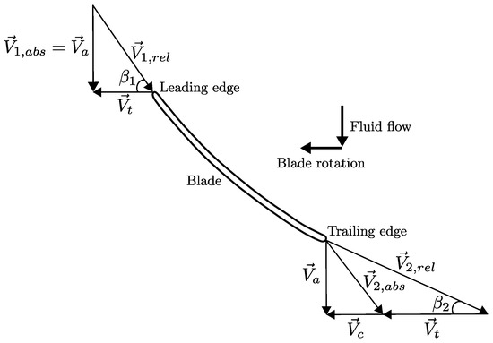
Figure 1.
Circular blade velocity triangle.
Before defining the blade angles, the following equations present the velocity magnitude definitions. Equation (1) defines the axial velocity derived from the continuity principle.
where Q is the flow rate (/s), A the annular area through which the fluid transits the turbine, and (m) are the turbine’s tip and hub radii, respectively.
The magnitude of tangential velocity is defined as the following product defined by Equation (2):
where (rad/s) is the angular velocity and r (m) the turbine’s radius.
The circumferential velocity is defined from the free vortex relation as shown by Equation (3).
Although k is not known at the beginning of a turbine design, it can be redefined in terms of known design parameters using the following definitions for mechanical power (Equations (4) and (5)) and the torque (Equation (6)) [30]:
where T (Nm) is the torque and the mass flow rate (kg/s).
In that regard, from Equation (4) through (6), the new definition for k is achieved as shown by Equation (7).
Then, substituting Equation (7) into (3) we could obtain the circumferential velocity as a function of known parameters defined by Equation (8).
Once the velocity vectors are known, the blade angles and can be determined with Equations (9) and (10), respectively.
Additional parameters are used to quantify the hydraulic performance of the turbine. The first one is the head pressure drop generated by the turbine. This is defined Equation (11) and its units are meters of water column (mwc).
where and are the total pressures (Pa) of two different reference points. Point 1 corresponds to the fluid inlet to the turbine and point 2 to the outlet. In the denominator is the specific gravity of the working fluid , where is the fluid’s density (kg/).
Next, Equation (12) defines the Ansys CFX solver’s mechanical torque computed during the CFD simulations.
where S represents the rotational surfaces (the turbine blades), is the position vector, is the total stress tensor (pressure and viscous stresses), is the unit vector normal to the rotational surface, and is the unit vector parallel to the rotational axis [48].
The hydraulic power is the energy contained by the fluid in motion, which is transformed by the turbine into mechanical energy. This is defined by Equation (13).
where the hydraulic power can be rewritten in terms of the mass flow because (kg/s).
The turbine hydraulic efficiency is the ratio of output power to input power. For a turbine, the output power is and the input power is . Thus, using Equations (4) and (13), the efficiency of a hydraulic turbine can be computed as shown in Equation (14).
An important parameter to define a turbine’s hydrodynamic performance is the pressure coefficient . It represents the ratio between the pressure difference and the dynamic pressure. is defined by Equation (15).
where is the static pressure on the blade surface and , , and are the far-field pressure, density, and velocity, respectively.
2.3. Design Methodology
The circular blade geometry design considered the recommendations in Ramos et al. [34]. This methodology uses Cartesian coordinates in a two-dimensional plane for the geometric construction of the blade, see Figure 2. Figure 2a shows a front view in the -plane of a turbine schematic. The inner circumference with radius called “hub” represents the physical location where the blades meet the turbine body. The outer circumference with radius called “tip” represents the final physical extension of the blade. The annular area A located between the casing and the blade tip also called the area swept by the turbine is the area through which the fluid flows through the turbine. Additionally, the location of the design points along the radial coordinate r of one of the blades can also be observed. The wrap angle defines the blade span and the horizontal length L.
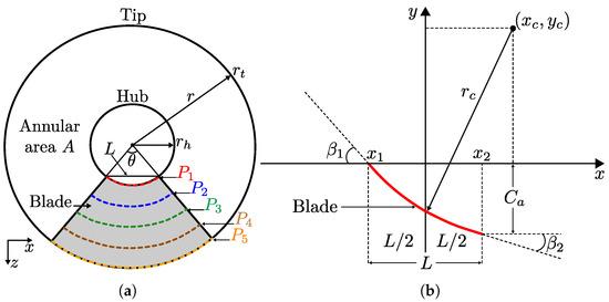
Figure 2.
Circular blade design’s schematic visualization. (a) Turbine’s frontal view where the design points are located at the radial coordinate r. (b) Geometric parameters defining the circular blade geometry. Modified from [34].
Moreover, the design points are defined based on the blade geometrical parameters shown in Figure 2b through a two-dimensional reference frame in the -plane. The blade can be seen in red, which has a geometry based on the arcs defined by the design points shown in Figure 2a. The geometrical parameters of the arc are as follows: represents the blade’s leading edge (fluid inlet), represents the trailing edge of the blade (fluid outlet), and L is the horizontal distance between and . The angles and are the blade’s leading and trailing angles. The coordinates and are the center of the arc. The length is the radius of the arc representing the distance from the center of the arc located at to the blade. Finally, is the blade axial chord measured from the x-axis to the trailing edge vertically. This length is paramount for turbine design because it defines the blade pitch as it meets the turbine casing at radius .
Now, the circular blade’s characteristic equations can be defined as follows. Firstly, the blade profile geometry could be obtained for five design points ranging from to . The P values are calculated using Equation (16).
where are the different design points to generate the blade profile along the radial coordinate r. are the hub and tip radii. is the increment distance to obtain the next design point. However, we chose to perform the blade design for three points because it is sufficient to generate the blade profile while keeping a simple design process.
The length L relates the design point and the wrap angle , as shown by Equation (17). Then, it is possible to determine the and using Equation (18).
The radius defining the distance from the arc’s center to the blade is a function of the length L and the blade angles and , as shown by Equation (19). Then, the arc’s center coordinates and can be computed with Equations (20) and (21).
The blade’s axial chord length is defined in Equation (22). Figure 2b shows geometrically where is located.
We obtained the circular blade geometrical parameters using the design parameters reported in Table 2. The free-vortex constant was /s (see Equation (7)) and a wrap angle . The wrap angle was obtained by computing , so the turbine blades could cover the annular area completely. Table 3 reports the circular geometric parameters obtained by using Equations (1)–(22) for design points , and .
Table 3.
Circular blade geometric parameters for a free vortex constant /s and a wrap angle .
The Cartesian coordinates and that describe the blade geometry curves are defined in Equations (23) and (24). These equations are based on the definition of a non-centered circumference.
where are the arc’s coordinate position and radius, respectively. The subscript “i” represents an nth point of the coordinates parametrization. Moreover, the parameters and are used to parametrize the blade curves at the nth points.
2.3.1. Coordinates Transformation
Ansys BladeGen was employed to create the 3D model of the circular blade. The strength of BladeGen resides in its capability to produce three-dimensional turbomachine blade models based on two-dimensional meridional coordinates. However, the designer must be familiar with these coordinates because they are distinct from Cartesian coordinates. This process involves converting from two-dimensional coordinates to cylindrical ones, then to three-dimensional coordinates, and ultimately acquiring the necessary meridional coordinates.
The process begins by transforming the two-dimensional Cartesian coordinates defined in Equations (23) and (24) into cylindrical coordinates . This transformation is performed using Equations (25)–(27).
where is the radial cylindrical coordinate equivalent to the hub, medium, or tip radii , respectively. The medium turbine radius can be determined as . The angular coordinate is computed from the definition of the length of an arc, where is the horizontal Cartesian coordinate of the blade, see Equation (23). Lastly, is the longitudinal cylindrical coordinate, where corresponds to the vertical Cartesian coordinate of the blade, see Equation (24).
Once the cylindrical coordinates are obtained, they are transformed into 3D coordinates using Equations (28)–(30).
where are the radial, angular, and longitudinal cylindrical coordinates, respectively.
Finally, the three-dimensional coordinates are transformed into the meridional coordinate system . The meridional coordinates correspond to a curved reference system used by Ansys BladeGen to generate blade geometries for various turbomachines. Chen et al. [49] have given in their study a good explanation of the meridional coordinate system using a Francis turbine as an example. In this manner, Equations (31)–(34) are used to obtain the meridional coordinates.
where the subscript i represents the i-th node located on the “spatial relative streamline (SSL)”, see [49]. denotes the three-dimensional coordinates on the i-th node in the Cartesian system. represents the i-th node in the meridional (curved) system. are the origin coordinates of the meridional system, which are assumed to be zero, i.e., . and are the axial and radial intervals of the adjacent nodes, respectively.
Lastly, a polynomial regression is applied to the meridional coordinates to determine the values at the position of . We checked if the coefficient of determination . If not, the grade of the polynomial regression should be increased. We found suitable results for a fourth-degree polynomial.
Figure 3 shows graphically the circular blade’s coordinates transformation process. The two-dimensional, three-dimensional, and meridional coordinates are shown in Figure 3a–c, respectively. For each coordinate system, the circular blade design points were generated at , which correspond, respectively, to the turbine’s hub , medium , and tip radii. Specifically for the meridional coordinates seen in Figure 3c, we made sure that the final values of at corresponded to because it was a design restriction imposed by the wrap angle .
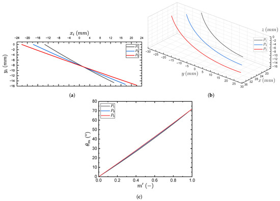
Figure 3.
Circular blade’s coordinate transformation process for design points . (a) Two-dimensional projection. (b) Three-dimensional projection. (c) Meridional coordinates.
2.3.2. BladeGen Geometry Generation
This subsection presents the circular blade’s 3D model using Ansys BladeGen. Figure 4 shows different design modules encountered within BladeGen. Figure 4A presents the three-dimensional turbine model, which indicates the fluid inlet and outlet, the blades’ location, and the front bulb’s simplification. We validate this simplification in the results section. In Figure 4B, module (a) corresponds to the meridional view that defines the turbine’s control volume and the blade boundaries from the leading edge to the trailing edge. We describe the meridional view in detail in Figure 5. In module (b), the blade-to-blade view, also called the cascade configuration, is observed. In this view are present two blade profiles with their curvature and thickness. Next, module (c) is of utmost significance in obtaining the blade geometry because the meridional coordinates obtained in the coordinate transformation process described above are inputted in this section. The x and y-axes corresponding to the coordinates and can be visualized, where is represented in blue color. Additionally, the function of the angle (in green), which corresponds to the blade inclination measured from the axial direction of the flow, can be observed. To clarify section (c), only the coordinates and are modified because the angle is automatically calculated according to the aforementioned meridional coordinates. For the last module (d), the blade thickness (in red) is defined with a constant value of 1.7 mm according to previous studies [6,34].

Figure 4.
(A) Three-dimensional model of the turbine. (B) BladeGen design modules.
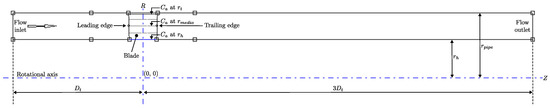
Figure 5.
BladeGen’s meridional view of the circular blade’s control volume (flow passage).
Figure 5 shows the meridional view coordinates used in the validation study to define the control volume, also called the flow passage. In BladeGen, the meridional view coordinates are , where Z is the axial coordinate (horizontal direction), and R is the radial coordinate (vertical direction). The domain of is and , respectively. The meridional profile of the blade is bounded by the leading and trailing edge lines defined by , see Equation (22). In the meridional view, this distance is defined in the Z coordinate for each design radius . For this type of blade, increases from radius to . It should be clarified that the blade is designed up to the turbine’s outer radius and not up to . The horizontal line located at represents the pipe wall and the turbine’s hub wall. Additionally, to ensure a developed flow, the inlet was located at a distance of one turbine diameter measured from the vertical R coordinate and the fluid’s outlet at . These lengths were based on the experimental setup of the reference study to perform the numerical validation [34].
3. Fluid–Structure Interaction (FSI) Simulations
This section describes the general methodology to carry out the fluid–structure parametric simulations. Then, we present the control volume discretization, the CFD boundary conditions, and the parametric fluid dynamic simulations. Lastly, we show the methodology to perform the static and dynamic structural parametric simulations.
3.1. Proposed Methodology
Figure 6 shows the methodology we proposed to perform the one-way fluid–structure interaction (FSI) simulations to investigate the circular blade. The methodology was divided into four main phases: the first consisted of the discretization of the control volumes and the mesh study (quantification of the mesh uncertainty). The second phase corresponded to the CFD fluid dynamic parametric simulations. In the third phase, static structural parametric simulations were developed. Finally, the fourth phase included the dynamic structural simulations corresponding to the modal analysis and harmonic response. The following is a general description of each phase of the methodology.
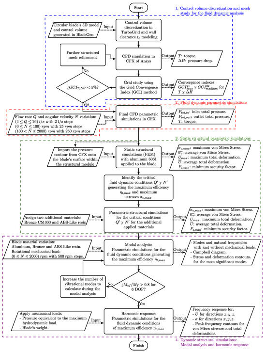
Figure 6.
Proposed methodology for the one-way fluid–structure interaction (FSI) parametric simulations.
In the first phase, the mesh for the circular blade’s control volume was generated in the meshing module Ansys TurboGrid. In TurboGrid, the blade clearance mm was created according to the design parameters, see Table 2. The blade clearance is essential to model the losses generated by tip leakage vortices to avoid overestimating the hydraulic efficiency of the turbine. Then, the meshes were transferred to Ansys CFX, where a working condition was simulated to obtain the results of torque T and pressure drop . With these results, we performed the mesh study by applying the Grid Convergence Index (GCI) method [50]. The results of the mesh study are the convergence indexes for the fine and medium meshes and , respectively. We checked if one of them was below 5% to select the mesh. If not, the mesh was refined again.
The second phase corresponds to the final parametric CFD fluid dynamic simulations in CFX. The fluid dynamic and turbulence model governing equations are presented in Appendix A. On the one hand, the variable input parameters are the flow rate Q of the working fluid (water at ambient temperature) and the turbine angular velocity N. The flow rate varies over a range of l/s with steps of 2 l/s. This range corresponds to the capacity of the hydraulic test bench available in our laboratory. Following, N varies in two ranges: the first corresponds to rpm with steps of 25 rpm and the second is rpm with steps of 250 rpm. On the other hand, the output parameters are the total inlet and outlet pressures and , respectively, and the turbine torque T.
In the third phase, static structural parametric simulations were carried out. The static structural governing equations are presented in Appendix B.1. The pressure contour on the wall of the circular blade was imported from CFX into the Ansys static structural module. The output parameters of the static structural simulations were the maximum von Mises stress and average , the maximum total deformation and average , and the minimum safety factor . During the static structural simulations, the aluminum 6061 material was assigned to the circular blade. The next step was to identify the corresponding fluid dynamic working conditions for flow rate and angular velocity, renamed as and , respectively, which generated the results of , , , and the maximum turbine hydraulic efficiency . This was done to configure additional static structural parametric simulations, which had two additional materials as bronze and ABS-like resin.
Lastly, the fourth phase corresponds to dynamic structural simulations that include modal and harmonic response analyses, whose governing equations are presented in Appendix B.2 and Appendix B.3, respectively. For the modal analysis, we varied the blade material using aluminum, bronze, and ABS-like resin for the fluid dynamic conditions that generate . Then, we determined the variation of mode natural frequencies a function of turbine rotational speed in a range of rpm with steps of 500 rpm. In this way, we evaluated the relationship between natural frequencies and the rotational speed of the structure, and the result is the so-called “Campbell diagram”. To achieve this, the parameter determining the number of calculated modes is the ratio of effective mass to total mass . We checked if , as recommended by Ansys [51], to decide on the amount of mode shapes to be calculated. The output parameters are the modes shapes and their natural frequencies with and without mechanical loads, the Campbell diagram, and the stress and deformation contours. For the harmonic response analysis, the mechanical loads of the maximum hydrodynamic pressure on the blade surface determined in the corresponding static structural analysis were applied as boundary conditions, along with a force corresponding to the weight of the blade. In this manner, these sinusoidal-varying mechanical loads were simulated harmonically to evaluate fatigue effects on the structure for the hydrodynamic conditions that generate . The output parameters are the frequency response of total deformation U and the normal stress in the x, y, z directions, as well as the von Mises stress and total deformation contours corresponding to the identified maximum frequency peaks in the frequency responses of the structure.
3.2. CFD Parametric Simulations
This subsection covers the first and second phases presented in Figure 6 related to the mesh discretization/mesh study and the final fluid dynamic parametric simulations. The first and second phases are presented in Section 3.2.1 and Section 3.2.2, respectively.
3.2.1. Spatial Discretization
Figure 7 shows the mesh refinement of the circular blade. Figure 7a–c show the fine , medium , and coarse meshes, respectively. The number of cells for each mesh size is given. Additionally, only the area of the control volume passage in meridional coordinates is shown, so it is visualized in two-dimensional form. Thus, it is possible to appreciate the refinement details of the meshes around the blade where, in general, the refinement is more important. From the three meshes, it can be seen that the change in refinement near the blade walls is not easily identifiable. However, the refinement of this zone, which corresponds to the inflation layers, correspond, respectively, to the fine, medium, and coarse meshes to a distance of the first cell of mm.
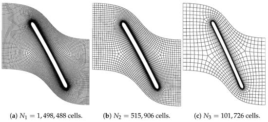
Figure 7.
Circular blade’s mesh refinement. (a) Fine , (b) medium , (c) and coarse meshes.
Once we generated the different mesh refinement levels, we applied the Grid Convergence Index (GCI) method whose equations can be found in [50]. Table 4 shows the results of the GCI study. The total number of cells for each mesh is reported. The refinement factors and satisfy the ASME recommendation concerning their lower limiting value, i.e., . Since , the apparent value p was calculated using a fixed-point iteration with an initial value . As for the response variables of the fluid dynamic solution, the pressure head , and the turbine torque T were selected. The selection of these parameters is because they are the main ones to determine the hydrodynamic performance of this type of turbomachine. For the numerical values obtained from the GCI study, a monotonic convergence was achieved because the ratio of the differences of the response variables is positive , and in turn, the apparent order also is . Concerning the theoretical order of the solution, which is related to the apparent order of the numerical solution p, it corresponded to the second-order (High-resolution) advection scheme used by CFX, i.e., . In general, apparent order p values for T and were close to the theoretical order of the fluid dynamic solution. The above is an indicator of the correct convergence of the meshes. However, the differences between the theoretical and numerical orders could be attributed to some shortcomings in the mesh quality, mesh refining, non-linearity of the solution, and turbulence modeling [52]. Despite this, these apparent orders do not invalidate the GCI methodology and are still acceptable for demonstrating mesh convergence. The approximate relative errors and the extrapolated relative errors were reported. These results indicate there are high relative errors greater than 13% for the coarse mesh. However, for the fine mesh, they are less than 3.2%. The extrapolated values , also called the Richardson extrapolation values, correspond to the asymptotic solution when the representative mesh size tends to zero , i.e., an infinitely refined mesh. Finally, the mesh convergence index GCI corresponding to the medium mesh was less than 3.15% for both T and . In contrast, the GCI for the coarse mesh exceeds 5%, which is considered high for proper convergence for the coarse mesh. Since a Mesh Convergence Index of less than 5% is considered within an acceptable threshold [53], the mesh selected was the medium mesh based on the result.
Table 4.
Mesh study results applying the Grid Convergence Index (GCI).
Figure 8 presents the mesh of the circular blade generated in TurboGrid, which consists exclusively of hexahedral elements. As a clarification, the reason only one blade is visible in the figure is that the turbine geometry was created in BladeGen, which allowed one-fifth of the control volume to be discretized because the turbine was designed with five blades. Thus, modeling a fraction of the turbine reduces the computational cost. Different details of the meshes can be seen. For example, in Figure 8a are the inflation layers on the walls of the control volume, i.e., on the pipe wall at the radius and the inner radius of the turbine. In Figure 8b is the surface mesh on the turbine walls, where details of the inflation layers are shown at the root and tip of the blade and , respectively.

Figure 8.
Medium-refined mesh used to perform the final CFD simulations. (a) Control volume mesh. (b) Mesh on turbine walls.
3.2.2. CFD Boundary Conditions and Parametric Study
Figure 9 shows the fluid dynamic boundary conditions used for the final simulations, which were applied to the control volume of the turbine with a circular blade. This image is intended to clarify the locations of the boundary conditions and some of their constant numerical values. For example, the entire control volume shown in the figure is called the “passage” or “R1”, which rotates around the Z-axis in the negative direction with a variable angular velocity N. This rotational domain is defined by the fluid inlet and outlet surfaces, which are assigned a constant total inlet pressure of = 97,805.7 Pa, and a variable outlet mass flow , respectively. The constant total inlet pressure was defined based on the results of Samora et al. [6] regarding the Thoma coefficient, which is related to the cavitation of a turbine. In their study, they found that for the evaluated flow rate , cavitation conditions did not occur if it was ensured an inlet pressure equivalent to 10 meters of water column (mwc). For such reasons, a total inlet pressure equivalent to 10 (mwc) was defined for the fluid dynamic simulations of the present work, taking into account that the density of water was assumed as kg/ at room temperature. The definition for the variable parameters is explained after Figure 9. On the other hand, the lateral surfaces were defined as a fluid–fluid interface (periodic 1 and periodic 2) of rotational periodicity around the Z-axis. Additionally, the physical walls of the control volume correspond to the blade surfaces, the turbine inner radius at , and the pipe wall at . For these walls, the no-slip boundary condition was assumed, which defines the velocity at the wall with a velocity equal to zero .
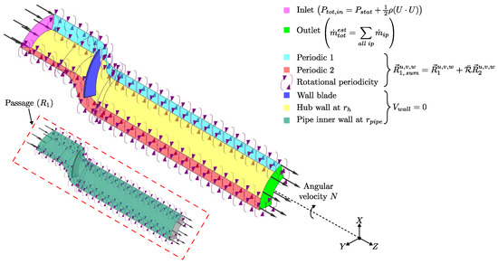
Figure 9.
CFD boundary conditions.
In the legend of Figure 9, we presented the fundamental mathematical definition of the boundary conditions. However, we describe them in more detail as follows:
The inlet is set to a subsonic total pressure boundary condition. It is defined mathematically as [48]:
where is the total pressure, is the static pressure, is the fluid’s density, and U the vector of velocity .
The outlet is set to a subsonic mass flow boundary condition. It is defined mathematically as [48]:
where the subscript “” stands for integration point, which locates each grid vertex. is the total estimated mass flow rate and are the density, area, and velocity, respectively, at each integration point.
Then, a scaling factor F is computed so the estimated mass flow rate at the integration points adds up to the specified mass flow rate .
Finally, during the computation of F, the new mass flow rate at each integration point is iteratively calculated as follows
The rotational periodicity boundary conditions are applied to the lateral surfaces of the control volume. The CFX solver of Ansys discretizes the turbulence model using a cell-vertex scheme [48]. Therefore, the mathematical definition of the rotational periodic boundary conditions is defined as [54]:
where the subscripts “1” and “2” are the two periodic boundary conditions set on the lateral surfaces of the control volume. The superscripts “” denote the three momentum equations. is the general vector for any physical quantity of the solution and is the rotation matrix defined as:
where is the angle between the periodic boundaries, which for the present paper is because one out of five blades is being modeled. Additionally, for our specific case, the control volume rotates about the z-axis.
Finally, the no-slip condition is applied to all walls. This means that fluid velocity at the walls is zero, i.e., .
Moreover, the fluid dynamic simulations were developed not only for one operating condition but also for a wide range of operating points. The parameters that varied to generate the different working conditions were the angular velocity of the turbine N and the discharge mass flow rate . First, N varied from 0 rpm to 100 rpm with steps of 25 rpm. Then, it continued from 250 to 2000 rpm with steps of 250 rpm. In total, the variation of N corresponded to 13 numerical values. As a clarification, the first range for N was implemented to capture in more detail the variation of turbine performance for low angular velocities, while the second one was used to cover a wide range. Second, varied for each N value from 0.798 kg/s to 5.184 kg/s with steps of 0.399 kg/s, that is, 12 values. Therefore, the total number of fluid dynamic working conditions simulated was 156.
The following equations were used to determine the numerical values for the boundary conditions used in the CFD simulations. Equation (41) shows how the inlet total pressure (Pa) was computed.
where m is the head pressure assumed at the inlet’s control volume, kg/ is the water density at room temperature, and m/ is the gravitational acceleration.
Equation (42) was used to calculate the outlet mass flow rate values .
where Q is the assumed inlet and outlet flow rate of the control volume. The range was /s with steps of /s. The above range was defined considering the capacity of our hydraulic test bench for future experimental studies. Lastly, the mass flow rate was divided by 5 because we modeled one-fifth of the entire control volume, for example, one of five turbine blades. The resulting value is known as the “passage mass flow rate”.
Concerning the CFX solver setup, the fluid dynamic parametric simulations were performed on a workstation with an Intel Xeon E5-2667 12-core 2.9 GHz processor and 32 GB of RAM. A steady-state analysis was used with a continuous fluid-type domain (water at 25 °C) used at a reference pressure of 1 atm. In the validation study, reported in Section 4.1, it was shown that there is no significant numerical difference for the fluid dynamic response variables obtained with a steady-state and transient analysis. For this reason, a stationary analysis was implemented. The turbulence model used is . This model correctly predicts the adverse pressure gradients on the sustaining surfaces of hydraulic turbines, which is why different authors have used this turbulence model for this type of simulation. The governing equations for the model can be found in Appendix A.2. The advection scheme was of second order, i.e., High Resolution. The convergence criterion was configured for the RMS residuals (Root Mean Square) with a magnitude of . This is because the most relevant convergence magnitude was identified taking into account the stability and convergence of the output variables, such as torque and total inlet and outlet pressures. Furthermore, it has been identified in different studies related to hydraulic turbine fluid dynamic simulations that the magnitude of convergence mentioned above is acceptable from an accuracy point of view, taking into account numerical errors [48].
Table 5 presents information on important parameters for CFD simulations from different studies of in-pipe turbines, the simulation regime, the turbulence model used to model the fluids’ governing equations, and the dimensionless wall distance are reported. Most studies’ simulations use a transient regime, the SST turbulence model, , and the ANSYS CFX fluid dynamics simulation module. The SST turbulence model was chosen due to its proven accuracy and robustness in predicting complex flow phenomena, particularly in boundary layer flows under adverse pressure gradients. This model combines the benefits of both the model in the near-wall region and the model in the free-stream region, making it highly effective for capturing the detailed flow characteristics around turbine blades. The SST model is less sensitive to the initial conditions and can handle a wide range of flow scenarios, which is relevant for accurately simulating the regimes observed in turbine operations within pipelines. Therefore, for developing the fluid dynamics simulations and following previous research recommendations, the SST turbulence model was selected for this problem.
Table 5.
CFD simulation parameters for in-pipe turbines used in different studies.
3.3. Structural Parametric Simulations
This subsection covers the third and fourth phases presented in Figure 6, namely, the static structural parametric simulations and the dynamic parametric simulations (modal and harmonic analyses). The methodology presented in this section was based on similar studies previously reported [12,22]. The static and dynamic structural governing equations can be found in Appendix B.
3.3.1. Static Structural
The materials considered for the structural parametric simulations are reported in Table 6. The materials used were aluminum alloy 6061-T6, bronze alloy C51000, and ABS-like resin. For each material, the mechanical properties were defined, where is the density, the coefficient of thermal expansion, the Poisson’s coefficient, E the Young’s modulus, G the shear modulus, the yield strength, and the ultimate stress. The mechanical properties of aluminum and bronze were determined with the Ansys Granta database [61], which is available in Ansys Workbench. On the other hand, the ABS-like resin’s mechanical properties were taken from the SUNLU manufacturer [62]. Aluminum and bronze were considered to evaluate the structural behavior of the blades because they are materials of interest for the manufacture of blades due to their mechanical characteristics suitable for fluid dynamic loads [63,64]. ABS-like resin can also be an alternative to the previous two materials because it is used by 3D resin printers with curing through UV light, which can facilitate manufacturing processes [65]. This manufacturing process is known as stereolithography, with which different types of blades have been successfully fabricated, such as turbine blades for aircraft engines [66]. In addition, the resin also has acceptable mechanical properties for fluid dynamic loads typical of turbomachinery in the hydraulic field [67].
Table 6.
Mechanical properties of the materials used in the structural simulations.
Regarding the boundary conditions used in the Ansys static structural module, fluid dynamic (pressure contours on the blade surface), centrifugal (turbine rotational speed), and gravitational mechanical loads were imposed. Figure 10a shows the pressure contour imported to the pressure surface of the circular blade. This data transfer is performed from the CFX results to the static structural module and is done using the “Mechanical-Based Mapping” algorithm, allowing us to interpolate the results of the pressure contour on the blade surface in question. Next, Figure 10b shows the additional boundary conditions used during the static structural simulation. As can be seen, a fixed support identified in the figure with the letter “A” was created at the root of the blade . This fixed support constrains the blade in its 6 degrees of freedom. Identified with the letter “B” are the surfaces on which the pressure contour imported from CFX shown in Figure 10a was applied. To take into account the weight of the blade due to the Earth’s gravity, and the centrifugal forces due to the angular velocity, “C” and “D” boundary conditions were applied, respectively. The numerical value of this boundary condition varies as an input parameter according to the rotational speed N of the turbine defined in Table 6.

Figure 10.
Structural boundary conditions. (a) Imported pressure contour from the CFD simulation into the static structural simulation. (b) Static structural boundary conditions.
To carry out the structural simulations, a mesh independence study was necessary. The goal was to find a number of nodes and cells of the blade mesh that capture the structural results within an acceptable limit. For this purpose, the “Convergence” tool offered by the Ansys static structural module was used. For the present study, it was decided that the mesh study and, therefore, the mesh refinement be performed for the von Mises stress results, also called “Equivalent stress”. In this way, the structural module evaluates whether or not the numerical value of the von Mises stress solution is within a permitted percentage change. Thus, the allowable percentage change selected was 10% [68]. The mesh convergence study is shown in Figure 11a for a specific fluid dynamic condition. Figure 11b shows a three-dimensional visualization of the meshed blade corresponding to the mesh refinement process. The most remarkable feature of this mesh study method is that the solid representing the blade is not refined uniformly throughout its volume, but the refinement takes effect in the localized zones where the gradient of the numerical values of the structural solution is higher; and for those zones where the gradient is lower, the refinement is lower. This can be visualized at the blade root, where the maximum stress values developed (see red label “max”). In contrast, the refinement is lower in the areas where the stress values do not change considerably (minimum values “min”). As a clarification, this process was performed for the 156 simulation points established for the FSI simulations.

Figure 11.
Structural mesh convergence study. (a) Structural refinement plot. (b) Refined structural mesh visualization.
3.3.2. Dynamic Structural
This section describes the methodology for developing dynamic structural simulations corresponding to modal and harmonic response analyses. Because these analyses are the last performed, Figure 12 shows the modular data flow in Ansys Workbench to develop the FSI fluid–structure simulations, specifically those to finalize the dynamic structural study corresponding to phase 4 of the general methodology presented previously in Figure 6. According to Figure 12, the results of the static structural analysis are used as a pre-configuration for the modal analysis. Two modules were used for the modal analysis. The first module was used to generate the Campbell diagram results for the evaluated materials. The second modal analysis module was used as the initial condition for the harmonic response analysis. Essentially, it was necessary to use two different modules for the modal analysis because, for the first module, Coriolis effects had to be activated to generate the Campbell diagram output. However, the harmonic response analysis is not compatible with the modal analysis module if the Coriolis effect setting is active. Therefore, the second modal analysis module had to be created without the Coriolis effect configuration to be used as input conditions for the harmonic response analysis. In the following, the configuration of the modules for modal and harmonic response analyses is described.

Figure 12.
Information flow in Ansys Workbench to complete the FSI simulations with modal and harmonic response analyses.
For the modal analysis, we used as input parameters the previously defined materials, the fluid dynamic conditions that generated and the variation of N varying from 0 rpm to 2000 rpm with steps of 500 rpm. As an output parameter, the number of modes to be calculated was defined. This value was selected based on the ratio between the effective mass and the total mass of each mode corresponding to its natural frequency. If for all six blade degrees of freedom (6 DOF), both translational and rotational , then the number of modes to be calculated in the modal analysis must be increased, and thus the modal analysis must be redone. Conversely, if , then a sufficient number of modes are considered to have been computed to determine the most significant modes of vibration of the structure. Finally, the Campbell diagram, and stress and strain contours for the most significant modes were also obtained. The same methodology was applied to the second module for modal analysis. However, the rotational mechanical load varying N was not used to create the initial conditions for the harmonic analysis.
For the harmonic response analysis, the solution of module 2 of the modal analysis was used to preconfigure the harmonic response analysis module. This was done to carry out the harmonic response simulations through the mode superposition method, which solves the governing equations [51] by applying the assigned mechanical loads harmonically, i.e., they vary sinusoidally. The mode superposition method creates additional modes based on the simulation of the previous modal analysis to calculate the response of the structure in the frequency domain. Hence, this method is faster and less computationally intensive compared to a full harmonic analysis [69]. The boundary conditions used for the present study are shown in Figure 13. First, Figure 13a shows the configuration tree of the harmonic response module in Ansys, where it is observed that the initial conditions correspond to the second module of the modal analysis (“Modal (Modal 2)”). Next, Figure 13b shows the applied mechanical loads corresponding to a pressure and a force. The pressure corresponded to the maximum hydrodynamic pressure detected for each blade according to the fluid dynamic simulation, and the applied force was the weight of each blade taking into account its mass. The pressure load was assigned on the blade surfaces except for the one where the blade is fixed, i.e., on the root of the blade corresponding to the inner radius of the turbine ; the force was assigned to the solid representing the blade. Additionally, in the “Analysis Settings” section presented in Figure 13a, a damping coefficient of 2% was assumed to avoid the frequency responses not matching with real results, thus avoiding incoherent or overestimated results. This was done based on the Ansys recommendation [69].

Figure 13.
Boundary conditions used in the harmonic response analysis. (a) Creation of the mechanical loading conditions of pressure and force, and generation of results. (b) Zones of application of mechanical loads on the blade.
Regarding the solution parameters of the harmonic response analysis, the frequency response of the total deformation U and of the normal stress in the directions were taken into account, as can be seen in the solution section “Solution” in Figure 13a. For each of the above results, the maximum value was specified to define the frequency range , which corresponded to a factor of the maximum natural frequency of the last mode calculated in the modal analysis. Thus, the frequency specified for each U and result is given by Equation (43).
where the 1.5 factor is recommended by Ansys to specify the maximum value for the frequency range to be determined in the frequency response results [69].
4. Results
This section is divided into three subsections. Section 4.1 presents the numerical model validation. Section 4.2 presents the fluid dynamic simulation results. Lastly, Section 4.3 compiles the static and dynamic structural results.
4.1. Numerical Model Validation
The objective of this section is to compare the turbine efficiency obtained from the numerical model with experimental results available in the literature. It also intends to compare the numerical results between steady state and transient simulations and compare them with the experimental results to determine the type of analysis to be used for the final fluid dynamic simulations. The validation study used the experimental results of Samora et al. [6]. However, the authors did not report the original design parameters with which they generated the turbine geometry under investigation. Therefore, for the present validation case, the design parameters of the turbine at the best efficiency point (BEP) were assumed based on the experimental results. Thus, Table 7 shows those experimental parameters at the BEP of the turbine from the study of Samora et al.
Table 7.
Turbine design parameters at the best efficiency point (BEP) for the numerical model validation based on the study of Samora et al. [6].
Figure 14 shows the turbine geometry obtained from the design parameters reported in Table 7. In Figure 14A is the 3D model of the turbine, where the blades and the fluid inlet and outlet are indicated. In the inlet region, a straight section up to the blades can be observed. It was decided to simplify the front bulb of the turbine because the hydraulic losses generated by it are negligible compared to those generated by the blades and the fluid section at the outlet [70]. The simplification of the bulb makes it easier to obtain acceptable quality metrics, in addition to reducing the total number of mesh elements. In the outlet section, there is a casing that physically contains the turbine shaft and has a radius equal to the turbine hub . This casing is geometrically modeled following the experimental setup of Samora et al., [6]. In Figure 14B are the design modules from (a) to (d), which were configured as explained in Section 2.3.2. As clarification, in module (c), the angle is represented in green color, and in blue. In module (c), the blade thickness of 1.7 mm is represented by the line in red.
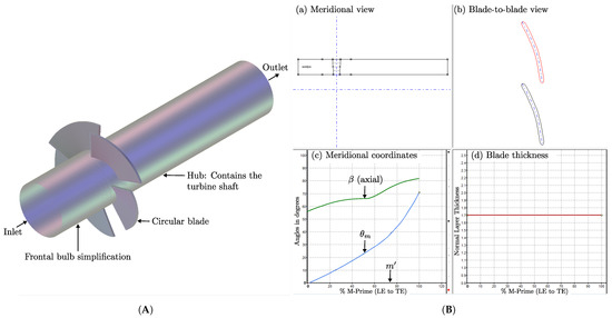
Figure 14.
BladeGen geometry generation for the experimental results of Samora et al. [6]. (A) Three-dimensional model of the turbine. (B) BladeGen design modules.
Table 8 shows the turbine geometric parameters consisting of the inlet and outlet angles and the two-dimensional coordinates that define the turbine blade at three design points at the inner , middle , and outer radii of the turbine. Once the geometry of the turbine is designed based on the experimental BEP, we performed a mesh study and applied the GCI method, as reported in Section 3.2.1. Then, we configured the CFX solver following the same methodology reported in Section 3.2.2.
Table 8.
Two-dimensional Cartesian coordinates of the blade for the validation study for a free-vortex constant /s and a wrap angle of .
4.1.1. Steady-State Analysis
The validation study had two goals. The first one was to evaluate the effect on the hydraulic efficiency of the turbine by varying four geometric parameters corresponding to the circular blade using a steady-state analysis. The second goal was to perform transient simulations and compare their results with the steady-state ones to decide which of the two analyses would be used in the final CFD simulations for this study.
The first two cases corresponded to the axial chord length of the blade, see Equation (22) for its definition. In theory, based on the meridional view of the blade in BladeGen, the correct horizontal length of each side of the meridional profile with respect to the R-axis is towards the leading edge, and towards the trailing edge, resulting in a total axial chord of , see Figure 15a. However, within the validation study, an additional case was considered for the definition of the axial chord length. This additional case corresponds to an axial chord length measured from the R axis to the leading and trailing edges for each side. That is, the total axial chord length is , see Figure 15b.
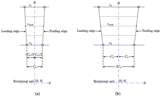
Figure 15.
Definition of the axial chord of the blade’s meridional profile measured with respect to the R-axis. (a) Case 1 for . (b) Case 2 for .
In BladeGen, the R-axis is located at the center of the blade’s meridional profile, see Figure 15. However, the axial chord is defined at the Z coordinate (horizontally) by varying the design radius with the radii , and . Therefore, Table 9 shows the axial chord lengths and for each design radius . The objectives were to study the influence on the turbine efficiency with the variation of the axial chords (cases 1 and 2), and to validate which axial distance is the correct one while comparing the numerical result to the experimental one to validate the numerical method. Finally, the location of and , was performed as follows: is located at the R coordinate and , are located at the Z coordinate.
Table 9.
Blade’s axial chord length cases as a function of the design radius .
We evaluated two additional cases concerning the modeling of the blade clearance . The blade clearance is the distance between the turbine blade’s external wall and the inner pipe wall. On the one hand, Figure 16a shows the clearance mm modeling. In this case, the working fluid passed between the pipe wall and the outer wall of the blade. This case corresponds to the actual physical operation of the turbine. On the other hand, Figure 16b shows the ideal case in which there is no blade clearance between the blade and the pipe, which means no hydraulic losses are generated. These hydraulic losses are known as tip leakage vortices.
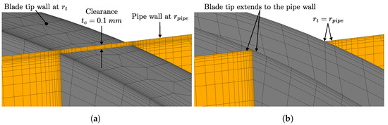
Figure 16.
Evaluated cases for the blade clearance. (a) Case 3 with clearance. (b) Case 4 no clearance.
Four fluid dynamic simulations were carried out combining the two cases of the blade axial chord and the two cases of the blade clearance modeling. According to Table 9 and Figure 16, the combinations between the axial chord and blade clearance are the following: (1) no clearance and . (2) No clearance and . (3) With clearance and . (4) With clearance and . Thus, Figure 17 shows the results of the hydraulic efficiency, calculated with Equation (14), for the four aforementioned cases. The horizontal line represents the experimental hydraulic efficiency of the turbine at point BEP , whose experimental data were obtained in the research of Samora et al., [6]. Concerning this value, the relative error of the numerical efficiencies for each case was calculated. According to the obtained results, the case that was closest to the experimental efficiency was case (4), which corresponds to modeling the blade clearance and an axial chord of . For this case, the relative error was , which is considered acceptable. The other cases have a relative error above 4%. This result indicates that the correct blade axial chord is , whose numerical value is presented in Table 9. On the other hand, if an axial chord of is used and the blade clearance is not modeled, this produces an overestimation of the efficiency by 4.35%. This is because it would be taking advantage of all the hydraulic energy available from the turbine generated by the maximum swept area of the blades inside the pipe. Therefore, it is imperative to take into account the blade clearance to ensure accurate CFD calculations.
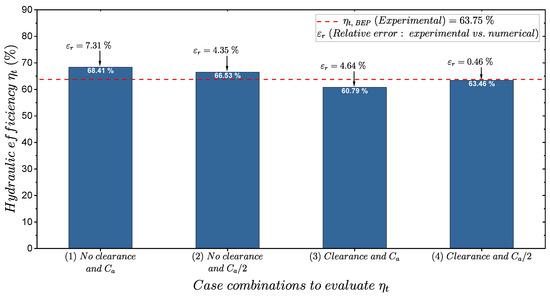
Figure 17.
Comparison of the hydraulic efficiency obtained through the CFD numerical model for different geometrical cases of the circular blade with respect to the experimental efficiency obtained from [6].
4.1.2. Transient Analysis
The transient CFD analysis was divided into two studies:
- The study of the influence of the time-step size on the numerical solution, where corresponds to the fraction of time of each iteration of the transient solution. With the obtained results, the temporal grid convergence index (GCI) method was applied to the time-step .
- The study of the influence of the total physical time of the transient simulation.
In the following, we present the results of the aforementioned transient studies:
- 1.
- Study of the influence of the time-step size :
The time-step size was determined using Equations (44) and (45).
where is the time-step size (s), is the number of turbine rotations, is the turbine angular velocity (rad/s), is the number of total iterations of the transient simulation, and is the angular rotation of turbine per iteration. , , and are input parameters for this study.
Table 10 presents the parameters selected to perform the time-step size study. The first input parameter was the degree of rotation of the turbine , for which four values were selected to cover a wide range from 20° to 1° of rotation per time-step size . As decreased, so did proportionally. The second input parameter was the number of turbine rotations, which was assumed with a constant value of . The reason was to keep the total simulation time invariant as the time-step size changed. The last input parameter was the angular velocity of the turbine, which corresponded to a constant value of rad/s (750 rpm). This value corresponded to the turbine’s design angular velocity of the experimental study, see Table 7. On the other hand, the output parameters were the size of the time-step , which was reduced due to the increase in the total number of iterations of the simulation. Finally, the total simulation time remained constant with a value of 0.32 s, which allowed us to isolate the influence of the change of on the numerical solution of the total simulation time . Thus, in the CFX-pre module, the simulation type was changed from stationary to transient, and the values of the time-step size and any of the values between the number of iterations or the total simulation time were used.
Table 10.
Parameters for studying the influence of time-step size on the transient simulation.
Table 11 presents the Grid Convergence Index (GCI) study applied to the time-step size . The numerical values selected for were s, s, s, from the most refined to the least refined, respectively. The response variables for the numerical solution were the pressure head and the turbine torque T. The apparent order p for the torque T and pressure head approximately equaled the theoretical order of the fluid dynamic solution, which corresponds to the second order (High resolution) advection scheme used by CFX, i.e., a numerical order of 2. The extrapolated values for T and resulted in 0.072502 Nm and 1.037424 m, respectively. These values correspond to the asymptotic solution when the representative mesh size tends to zero, i.e., for an infinitely small time-step size . Finally, the mesh convergence index GCI of for for T and was about 0.0048% and 0.0087%, respectively. In contrast, the GCI for for T and was 0.0057% and 0.0259%, respectively. According to the results, the selected time-step size was because its mesh convergence index was the lowest without drastically compromising the computational cost.
Table 11.
Results of the Grid Convergence Index (GCI) applied to the time-step size .
- 2.
- Study of the influence of the total physical time of the transient simulation:
Table 12 presents the parameters used to study the effect of the total physical time . The degree of rotation of the turbine is defined with a constant value of . This is because the result obtained from the GCI was applied to the time-step size (Table 10), which caused the time-step size to remain constant with a value of s. The number of rotations of the turbine varied from 2 to 8 with steps of 2. The angular velocity of the turbine was also kept constant. Then, using Equation (45), the number of iterations was obtained. Thus, the total physical time of simulation was calculated as .
Table 12.
Parameters for studying the influence of the total physical time .
Figure 18 shows the results of the study of the total physical time of the transient simulation. To give a more intuitive physical sense, the time can be represented through the number of turbine rotations , see Table 12. Thus, the independent variable of the graph corresponds to the number of rotations of the turbine . For the dependent variable, one can observe, from left to right, the values of the hydraulic efficiency , the relative percentage error between the numerical and experimental hydraulic efficiencies, and the wall-clock time to complete the simulation, respectively. The experimental efficiency of the turbine, represented by the horizontal line, corresponds to the best efficiency point (BEP) with a value of . According to the results, has an absolute variation of 0.05% with respect to the variation of the number of rotations ; the values of for and are 63.31% and 63.37%, respectively. Therefore, it is concluded that increasing the number of turbine rotations does not generate a significant change in the numerical hydraulic efficiency. On the other hand, the relative error between the numerical and experimental efficiencies for and is 0.68% and 0.6%, respectively. This result indicates that with the increase in the number of turbine rotations, the error with respect to the experimental efficiency value is reduced, but not significantly due to a percentage variation of about 0.03%. However, the wall-clock time (green line) required to complete the simulation does increase significantly. For these times values, there was a 49.3% increase between the corresponding values for (12.92 min) and (82.65 min). This increase in time is considered high considering that the change in hydraulic efficiency is minimal. Therefore, this result reaffirms that the transient simulation does not present significant differences compared to the steady-state analysis.
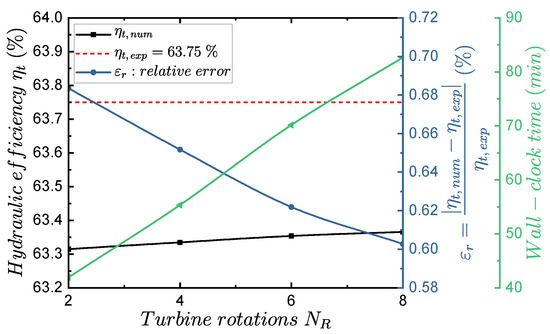
Figure 18.
Numerical transient-state hydraulic efficiency as a function of the number of total turbine rotations compared to the experimental efficiency at BEP obtained from [6].
To complete the validation study, Figure 19 shows the distribution on the suction and pressure surfaces of the blade for the dimensionless distance shown in Figure 19a and the pressure coefficient shown in Figure 19b. These distributions are a function of the dimensionless chord , where 0 and 1 correspond to the leading and trailing edges of the blade, respectively. For each blade surface, these quantities were calculated for the steady-state and transient solutions. According to this comparison, it can be observed that the distributions of and for the steady-state and transient solutions are almost the same with negligible differences. Thus, it is confirmed that there are no significant differences between the two different analyses. Therefore, it was decided to use a steady-state analysis for the final CFD simulations for the circular blade according to the methodology of the numerical model presented here.
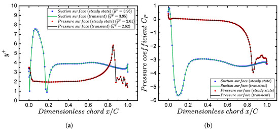
Figure 19.
Distribution comparison of (a) the dimensionless distance and (b) the pressure coefficient on the suction and pressure blade surfaces between the steady-state and transient analyses.
4.2. Fluid Dynamic Results
This subsection presents quantitative results of the fluid dynamic behavior of the circular blade relating to hydraulic parameters such as flow rate, pressure head, and hydraulic efficiency.
Figure 20 presents the hydraulic performance of the circular blade in terms of the flow rate Q. Figure 20a shows the flow rate values for which the turbine extracts energy from the fluid for a given angular velocity N. This means that the extension of the horizontal lines determined by the range of Q suggest torque generation behavior by the turbine. It was found that the blade was able to operate as a turbine for the full range of angular velocities evaluated (from 25 rpm to 2000 rpm) and with a decrease in the Q range to /s for 1750 rpm and 2000 rpm. Figure 20b shows the head pressure drop , see Equation (11), which represents the power energy consumed by the turbine to perform the energy transformation to mechanical energy. In general, for propeller-type turbines, is proportional to Q with an ascending quadratic trend. From the graph, it can be seen that the numerical values of decrease as the angular velocity N of the turbine increases. This is because, at high rotational speeds, the fluid perceives less obstruction due to better guiding of the fluid by the blade. The maximum head pressure drop m occurred for the maximum flow rate evaluated, i.e., /s at rpm. Figure 20c shows the mechanical power , see Equation (4), which behaved proportionally to Q and N with an ascending quadratic trend. increased gradually for the full range of N with no decrease in torque. Finally, the maximum mechanical power of 2364.72 W occurred at the maximum flow rate of /s at rpm. Figure 20d presents the hydraulic efficiency , see Equation (14). Some conditions developed an ascending curve that reached a maximum point and then descended again, which is expected for this kind of turbine. However, some curves did not exhibit the bell-shaped tendency but rather descended gradually as the flow Q increased. This means that the turbine operated under conditions of low rotational speed N, for which the maximum values of cannot be obtained. These conditions occurred for angular velocities rpm.
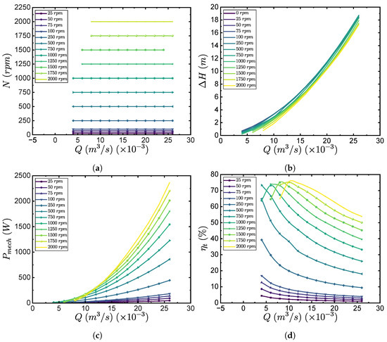
Figure 20.
Fluid dynamic performance of the circular blade as a function of the flow rate Q. (a) Angular velocity N. (b) Head pressure drop . (c) Mechanical power . (d) Hydraulic efficiency .
Figure 21 presents the best efficiency point (BEP) corresponding to the curves of hydraulic efficiency , pressure head , and mechanical power as a function of flow rate Q. The vertical line (in green) indicates the maximum efficiency and the corresponding values of pressure head and mechanical power. The maximum efficiency (whose function is in black) of occurred at a flow rate of /s. The pressure head (in red) and mechanical power (in blue) at the maximum efficiency were m and W, respectively. For the aforementioned values at the BEP point, it is possible to determine that the circular blade could operate efficiently, generating a considerable pressure drop and acceptable mechanical power considering that the turbine has a relatively small diameter of approximately 75 mm. However, it is discussed that the mechanical power plays an important role when it comes to the selection of the electrical generator to be paired with the turbine. The reason is because higher values of mechanical power facilitates the selection of the electric generator. Thus, according to the hydraulic performance of the circular blade, it could operate at the maximum values of , i.e., at rpm, while operating above 55% of efficiency for most of the flow rate Q, see Figure 20d.
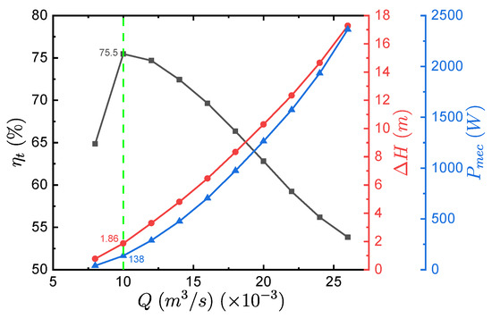
Figure 21.
Best efficiency point (BEP) of the circular blade.
Figure 22 allows for visualizing the behavior of hydraulic efficiency as a function of flow rate while relating it to different hydraulic variables using heat contours. It was identified that the maximum values of hydraulic efficiency were obtained for a flow rate range between 4 and for all the relationships presented. In this manner, Figure 22a shows the hydraulic efficiency as a function of flow rate Q and angular velocity N. It can be observed that the maximum values of hydraulic efficiency were obtained for angular velocities between 1000 and 2000 rpm. Figure 22b shows the hydraulic efficiency as a function of flow rate Q and pressure head . It was identified that the peak values of the efficiency were for pressure heads less than 5 m. Figure 22c presents the hydraulic efficiency as a function of flow rate Q and mechanical power . For this case, the maximum efficiency values can be achieved for a power range between 10 to 1000 W.

Figure 22.
Hydraulic efficiency hill charts as a function of (a) Flow rate Q and angular velocity N. (b) Flow rate Q and head pressure drop . (c) Flow rate Q and mechanical power .
Figure 23 shows the distribution of the dimensionless distance on the suction and pressure surfaces of the circular blade. The distribution of is a function of the dimensionless chord , where 0 and 1 represent the leading and trailing edges, respectively. For comparison purposes, the distribution also corresponded to the fluid dynamic conditions at the best efficiency point (BEP). Additionally, the distribution corresponding to the suction and pressure surfaces was calculated at the mean blade radius, i.e., . Regarding the numerical results of the distributions, it can be observed that close to the leading edge , the magnitude peaks occurred due to the fluid acceleration in this blade zone. Along the middle zone of the chord, i.e., , the values did not vary significantly. For a value of close to 1, sudden variations occurred for values in a downward manner. This is due to the decrease in fluid velocity in this zone. Finally, the magnitudes remained within an acceptable range for the turbulence model with a maximum average value of .

Figure 23.
(a) Dimensionless distance distributions on the suction and pressure surfaces of the blade at . (b) Pressure coefficient distributions on the suction and pressure surfaces of the blade at with its corresponding lift coefficient .
Figure 23b presents the distribution of the pressure coefficient at the mean blade radius over the suction and pressure surfaces. The pressure coefficient for each blade surface was calculated using Equation (15). On the one hand, the theoretical maximum positive value for the pressure coefficient was , which corresponds to the maximum total pressure on the blade surface, also known as stagnation pressure. On the other hand, the more negative the value of is, the more suction the blade generated for that surface, which generally corresponded to the suction surface. This means that the pressure field in the vicinity of the blade suction surface corresponded to negative relative pressures. The most negative values were located at the leading edge . This behavior is because of the increase in the fluid velocity at the suction surface, and, therefore, a sudden decrease in the local pressure was generated. Then, as the fluid advanced along the chord length, the local pressure on the suction surface gradually recovered as the fluid velocity decreases. The values on the pressure surface did not vary significantly as the fluid advanced through the mean values of the blade’s chord. However, the curves over the pressure surface experienced a sudden decrease near the trailing edge . This is because, at this blade location, the fluid traveling on the pressure surface experienced drag, and hence acceleration, caused by the fluid traveling on the suction surface. Thus, fluid velocity increased on the pressure surface near the leading edge due to the negative or low-pressure field on the suction surface. Finally, the area under the curve of the distributions for the suction and pressure surfaces corresponded to the lift coefficient , which was calculated using Equation (46).
4.3. Structural Results
4.3.1. Static Structural Results
We start by presenting the static structural parametric simulation results. In Figure 24 we present the structural response of the blade to a range of fluid dynamic conditions. The structural solutions were reported as a function of the flow rate Q and the angular velocity of the turbine N, including when the turbine was not rotating, that is, rpm. Figure 24a shows the the curves for the maximum von Mises stress . It was identified that is directly proportional with a quadratic trend to the increase in the flow rate Q. The above was expected because the increase in mass flow, and therefore, the increase in flow momentum, should increase the mechanical forces exerted on the blades due to the increase in fluid pressure. However, an inversely proportional behavior between , and the turbine angular velocity N occurred. This is because the fluid pressure is higher when the turbine is not rotating, which corresponds to the condition of higher torque production by the blades. Thus, once the turbine begins to rotate, the fluid guiding improves, and, therefore, the mechanical loads exerted by the fluid decrease. As a clarification, the curves for for some N conditions behaved in an oscillating manner. The above occurred for N = (25, 500, 1000, 1250, 1750) rpm. This behavior can be attributed to errors in the interpolation of the solution or to numerical instabilities inherent to the workstation where the results were obtained. The aforementioned is concluded because the general trend of corresponded, for most of the curves, to a trend proportional to Q and inversely proportional to N. Finally, the maximum stress identified occurred at MPa. Figure 24b shows the maximum values of total strain as a function of flow rate Q for different angular velocity conditions N. It was identified that, like the von Mises stress, is proportional to Q with a quadratic trend and inversely proportional to N. The maximum value of was mm when the turbine was not rotating ( rpm). Figure 24c shows the safety factor as a function of flow Q for different angular velocity N conditions. The safety factor for all structural simulations was calculated with respect to the yield stress. For the case of aluminum, this stress is MPa. Thus, was determined using Equation (47), where the maximum von Mises stress is related.
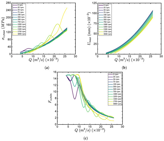
Figure 24.
Static structural parametric results of the circular blade as a function of the flow rate Q. (a) Maximum von Mises stress . (b) Maximum total deformation . (c) Minimum safety factor .
An important result regarding the safety factor is that its minimum values were not less than 1. This means the aluminum material could operate for all angular velocity ranges and flow rates. The aforementioned is because the maximum stress exerted on the latter is not greater than the yield stress. Therefore, the blade could not suffer permanent deformations. Finally, the minimum value of for the circular blade was = 1.11 for /s and rpm.
Figure 25a shows the maximum von Mises stress as a function of flow rate Q and angular velocity N. The maximum values of were found for angular velocities of rpm for a flow rate range of /s. Figure 25b shows as a function of Q and pressure head . The maximum values of occurred for the highest pressure heads m and flow rates /s. Figure 25c shows the peak strain as a function of flow rate Q and angular velocity N. It was identified that the peak values for were found over the entire range of angular velocities N for the maximum Q values. In Figure 25d is as a function of Q and the pressure head . In this contour, the same relationship was maintained, compared to the stress, of the peak values of located at the highest values of head pressure drop and flow rate Q. The hydraulic parameters at which these values occurred corresponded to rpm and /s. Lastly, Figure 25e shows the safety factor as a function of flow rate Q and angular velocity N. It can be seen from the contour that the maximum values of were maintained for values of /s and for the whole range of N. The minimum value of was approximately 1.1 for the maximum values of Q and N. Figure 25f shows as a function of Q and the head pressure drop . In this contour, it was evident that the maximum values corresponded to m and /s. For the rest of the Q range, decreased gradually with increasing values.
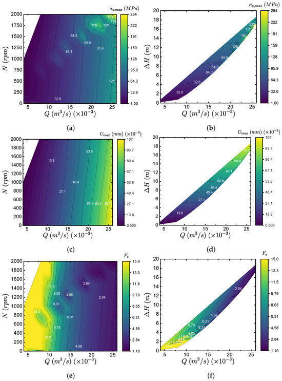
Figure 25.
Static structural hill charts. Von Mises stress , maximum total deformation , and minimum safety factor as a function of Q and N (a,c,e), and as a function of Q and (b,d,f), respectively.
Table 13 presents the identification of the fluid dynamic conditions that generated the maximum structural magnitudes for the evaluated materials, i.e., maximum hydraulic efficiency , maximum von Mises stress , the maximum total deformation , and the minimum safety factor . This was carried out according to phase 3 of the methodology presented in Figure 6. In the far left column are the aforementioned critical operating points. In the next three columns are the different materials evaluated and the fluid dynamic conditions , that generated the critical operating conditions. On the right side of the table are the numerical values of the von Mises stress , the total deformation U, and the safety factor . Concerning the obtained results, it can be observed that combinations between the different critical conditions were obtained. For example, “” means that the fluid dynamic conditions corresponding to and generated the maximum values of the maximum stress and deformation, and the minimum safety factor, respectively. Therefore, the combination between the critical conditions of and was expected to always exist because the factor of safety depends on the maximum stress, see Equation (47). Specifically for aluminum, only the combination of the critical conditions “” existed, thus, the fluid dynamic conditions , were different for the critical condition of . For the other materials, the combination of the critical conditions of “” also occurred. Next, for the safety factors, it was identified that they resulted in acceptable values for the highest efficiency conditions, i.e., with values of . However, there was a safety factor of 0.08 for the ABS-like resin material. This is attributed to the large stresses generated by the high-pressure head characteristic of the circular blade. This safety factor occurs when the turbine is static, i.e., not rotating, which is consistent with the maximum pressure head results.
Table 13.
Structural results corresponding to the critical fluid dynamic conditions and as a function of the material type.
Table 14 compiles the contours of von Mises stress and total deformation U for the circular blade’s critical conditions of maximum hydraulic efficiency as a function of aluminum, bronze, and ABS-like resin materials. These contours correspond directly to the fluid dynamic conditions and shown in Table 13. Concerning the visualization of the contours, the visible surface corresponds to the pressure surface, and thus, the fluid direction is toward the page. The suction surface of the blades is at the back side (not visible in the contours). The maximum values of the von Mises stress contour for the critical condition were located at the bottom edge of the blade for all materials. This is because, at the blade’s root, there is a sharp junction between the blade and the turbine body, leading to stress concentration.
Table 14.
Contours of von Mises stress and total deformation U for the critical condition of maximum hydraulic efficiency as a function of aluminum, bronze, and ABS materials.
In reference to the total deformation contours U, it was identified that the maximum values were located at the blade tip. This is attributed to the forces applied on the blade that produces higher bending as the radial length increases. It was also identified that the maximum values of U were located near the leading edge of the blade. This happened because the largest pressure gradients are generated at the leading edge due to the sudden change in fluid velocity as it transitions from the pressure surface to the suction surface.
4.3.2. Dynamic Structural Results
This subsection presents the dynamic structural parametric simulation results using the modal and harmonic response analyses.
- Modal analysis
The modal analysis was carried out for conditions and that generated the critical operating condition corresponding to the maximum hydraulic efficiency . These hydraulic conditions are reported in Table 13. The first result of the modal analysis is the determination of the number of vibration modes and its natural frequencies.
Figure 26 shows the modes and the natural frequencies as a function of the bronze, ABS-like resin, and aluminum materials corresponding to the circular blade. The number of significant modes was determined from the sum of the masses affected by the vibrations of the natural frequencies of the six degrees of freedom corresponding to the translational and rotational directions. When the sum was greater than 0.8, the number of significant modes of vibration was assumed to be acceptable [71]. The number of significant modes was 20 for each material. A larger number of significant modes of vibration indicates that there are more possible ways in which vibration energy can be distributed and transmitted in the structure during an external dynamic excitation by a mechanical load. This implies that there may be a lower risk of damaging resonances within the structure since there is a lower probability that the excitation frequencies will exactly match the natural frequencies of the structure, which could lead to excessive vibration amplitudes and possible failures. During the modal analysis, the natural frequencies with and without mechanical loads were determined. This can be differentiated according to the colors of the bars in the graphs. First, the natural frequencies, when there is no mechanical load exerted on the blades, are the frequencies at which the structure vibrates when it is not subjected to any external force or load. These frequencies are fundamental because they represent the inherent vibration characteristics of the structure and can influence its dynamic behavior when affected by external loads, in this case, hydrodynamic and rotational loads. Second, once the mechanical loads were applied, the natural frequencies changed and were higher than the unloaded natural frequencies. This is because mechanical loads alter the mass distribution and stiffness of the structure, which in turn affects the natural frequencies and vibration modes. Therefore, due to the considerable difference between the frequencies with and without load, it could be concluded that it is not plausible that the frequencies generated by the mechanical loads match the natural frequencies without loads. Therefore, within the evaluated fluid dynamic range, the circular blade could operate safely without presenting resonance phenomena and high vibration levels that could generate structural failures.
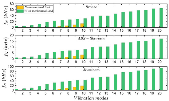
Figure 26.
Vibration modes and their corresponding natural frequencies as a function of the materials bronze, ABS-like resin, and aluminum.
Finally, referring to the magnitudes of the frequencies, the aluminum material obtained the highest frequencies for each vibration mode. The higher the frequencies between the vibration modes with and without load, the lower the possibility of blade resonance. Therefore, ABS-like resin could have a higher possibility of presenting this type of vibrational phenomenon, and in the same ascending order, bronze and aluminum. In contrast, the numerical values of the unloaded natural frequencies were relatively low compared to the loaded frequencies.
The Campbell diagram is a tool used in structural analysis, specifically for vibration analysis. It is normally applied to rotating machinery, which in this case corresponds to the blades that make up the propeller-type turbine investigated. In this context, the Campbell diagram relates the natural frequencies of the blades as a function of their rotational speed. In this way, it is possible to know how the natural frequencies of the vibration modes vary when the rotational speed of the turbine varies. The purpose of the Campbell diagram is to identify the resonance conditions between the natural frequencies corresponding to the blade modes of vibration and the rotational speed range of the turbine. Because resonance can produce damaging stress and strain amplitudes on the blades, it is important to identify which rotational speeds or multiples of them, known as the harmonics of the rotational speed, generate such resonances when these frequencies coincide with the frequencies of the modes of vibration. Therefore, knowing these conditions, one can identify safe operating ranges, conclude whether resonance conditions are not plausible to occur, or make decisions regarding the redesign of the structure under investigation.
Figure 27 presents the results of the Campbell diagrams of the circular blade as a function of bronze, ABS-like resin, and aluminum materials. In the Campbell diagrams, one can observe the natural frequencies (with mechanical loads) of the vibration modes on the vertical axis represented by green-colored lines. The total number of these lines corresponds to the number of significant modes defined in Figure 26. On the horizontal axis are both the rotational frequency (Hz) and the rotational velocity N (rpm). The numerical values of the rotational frequency were obtained from the relation s. In this way, it is possible to relate the rotational speed of the turbine in rpm to the natural frequencies of the vibration modes in Hz. Next, the straight lines in black color represent the multiples of the angular frequency , also known as the harmonics of the rotational velocity. Additionally, the maximum value corresponding to the multiples of was calculated to be greater than the natural frequency of the last mode of vibration. This is because the natural frequencies of the last mode are relatively high, thus providing a wide range for calculating the harmonics of . Additionally, the vertical line in blue represents the rotational velocity at which the blade operated at maximum hydraulic efficiency . Finally, the critical velocities were represented by the red asterisks. The critical velocities occur when there is an intersection between the curves of the natural frequencies of the vibration modes , the straight lines of the multiples/harmonics of the rotational frequency , and the straight line representing the rotational velocity of the maximum hydraulic efficiency achieved by the blade .
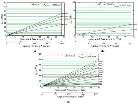
Figure 27.
Campbell diagrams corresponding to the circular blade for materials (a) bronze, (b) ABS-like resin, and (c) aluminum.
An important conclusion concerning the Campbell diagrams is that the natural frequencies corresponding to the vibration modes (green lines) did not vary significantly concerning increasing angular frequency . The above occurred for all three evaluated materials. This means that the blade operated at sufficiently low angular velocities to not affect the natural frequencies of the modes of vibration under the imposed hydrodynamic and mechanical loads. This fact is attributed to the relatively small dimensions of the blade (75 mm diameter rotor) because the vibration frequencies for relatively small structures are much higher compared to larger structures. For example, the natural frequencies of a blade corresponding to a hydro-kinetic turbine with a diameter of 1580 mm do not exceed 700 Hz [12]; this is compared to the maximum natural frequencies obtained in the order of 90 kHz for the circular blade studied. As a clarification, the fact that the natural frequencies of the corresponding vibration modes did not vary significantly with respect to the change of the turbine angular velocity is not an advantageous or disadvantageous result but corresponds to the identified intrinsic behavior. An advantageous fact for the structural integrity of the blade is the high magnitudes of the natural frequencies due to the relatively small sizing. The above is because the multiples of are close to or greater than a magnitude of units of a thousand, so that the excitation of the modes, and hence possible excessive resonances and vibrations are unlikely to occur for the high frequencies.
However, taking the above into account, it can be observed that some materials had a higher number of critical velocities compared to others. For example, the highest number of critical velocities corresponded to aluminum with a total of 12. One of the reasons for this situation is that the circular blade operated with the highest efficiency at 2000 rpm, so the multiples of could cover the whole range of the natural frequencies of the modes. All of the above conclude that the more critical speeds there are, the more susceptible the natural frequencies of the blade modes are to being excited by the frequencies of the harmonics derived from the rotational speed. But, the multiples of the rotational frequency are very large, e.g., the minimum value of the multiples of the rotational frequencies was for ABS-like resin. This implies that for the hydraulic conditions evaluated, the blade is unlikely to have resonances due to the high values of .
- Harmonic analysis
To conclude the dynamic structural analysis, we obtained the harmonic response using the mode superposition method. The objective of the harmonic response analysis was to determine the structural response of the blades from the sinusoidal variation of the hydrodynamic and mechanical loads exerted on the blades. In this way, it was possible to determine whether or not the circular blade subjected to sustained dynamic loads generates resonance and fatigue conditions due to the damaging effects of vibrations.
Figure 28 presents the frequency response function of the circular blade for bronze, ABS-like resin, and aluminum materials. On the vertical axis is the harmonic response of the directional deformation U (top of the figures) and the directional normal stress (bottom part of the figures). These harmonic responses were generated as a function of the evaluated frequency range . As can be seen in each figure, the range of varied for each material. This is because the range of to carry out the harmonic response analysis corresponds to a fraction of the maximum natural frequency of the vibration mode for each material. Therefore, Equation (43) was used to determine the range of . The above is recommended by the Ansys user’s manual [51]. Finally, the objective of plotting the harmonic response was to identify the location in the frequency of the maximum amplitudes of both U and , to identify possible resonances with the frequencies of the vibration modes, and to generate the contours of U and for the identified maximum frequencies. For this matter, the three Cartesian components corresponding to the directional deformation variables U and directional normal stress are also shown. Thus, for each of the graphs, a vertical line was generated to indicate the maximum values of U and , and their corresponding location within the frequency range (horizontal axis).

Figure 28.
Frequency response function of the circular blade for directional deformation U (top) and directional normal stress (bottom) corresponding to materials (a) bronze, (b) ABS-like resin, and (c) aluminum.
Table 15 shows the contours of the total deformation U and the von Mises stress corresponding to the maximum values identified in Figure 28. The left column shows the materials corresponding to bronze, ABS resin, and aluminum. For these materials, the total strain contours U and von Mises stress corresponding to frequencies , and , respectively, were generated with their corresponding phase angles . It was identified that the total deformation resonance conditions may exist because the frequency at which the maximum amplitude of the total deformation U occurs is close to the first mode of vibration (for bronze and ABS-like resin) and for the second mode of vibration (for aluminum). Concerning the stress contours, it was identified that the magnitude of the frequency at which the maximum stress values were generated coincides with the thirteenth mode of vibration. Additionally, it was identified that for all materials, the phase angles were negative, meaning that the structural response of the circular blade lags the input mechanical loads. In other words, the input mechanical loads reached the peak amplitudes first before the structural response of the blade. This is attributed to the damping factor assigned to the materials, which caused the harmonic response to be delayed with respect to the input excitation force. The damping factor assigned to all the materials was , which is a recommended value when its exact magnitude is not known for the material in question. Moreover, it is recommended to assign a damping factor for this type of simulation to avoid results that do not make physical sense [69].
Table 15.
Harmonic response contours of total deformation U and von Mises stress corresponding to frequencies and of the circular blade as a function of bronze, ABS-like resin and aluminum materials.
Finally, although coincidences were identified between the magnitudes of the frequency response and the natural frequencies of the materials, it was concluded that fatigue conditions did not exist for any of the three materials evaluated. This is because the maximum values of von Mises stress were well below the yield stress for all materials. For example, the yield stresses for the bronze, ABS resin, and aluminum materials were 505 MPa, 34 MPa, and 280 MPa, respectively. Thus, when compared to the maximum von Mises stresses of the contours, it can be concluded that for all materials operating under continuous harmonic loading conditions would not be at risk of permanent deformation. Therefore, no fatigue conditions can develop.
5. Conclusions
In this work, we design a turbine blade with constant curvature and thickness, known as a “circular” blade. It is designed based on the following hydraulic parameters selected from the review of the state of the art and the capacity of our hydraulic test bench: a flow rate of 15 l/s, a pressure head of 3 m, a hydraulic efficiency of 65%, and an angular velocity of 3600 rpm are assumed. The conventional one-dimensional design method is used with the free-vortex condition applied to the blade trailing edge. A mathematical methodology for generating two-dimensional Cartesian coordinates based on the design parameters is proposed to obtain the geometrical model of the blade. Then, a coordinate transformation process is used to obtain the meridional coordinates with which the three-dimensional geometry of the blade is generated in the BladeGen module of ANSYS. We contribute to the scientific community by openly sharing the source code used to generate the meridional coordinates of the circular blade and by automatically applying the Grid Convergence Index method to perform the mesh study.
To perform the FSI fluid–structural fluid dynamic simulations, the fluid dynamic numerical model used in this research is validated concerning the experimental results of Samora et al. [6]. The numerical model is satisfactorily validated because there is a 0.46% relative error between the numerical and experimental hydraulic efficiency. The results of the CFD simulations evaluated a flow range from 2 to 26 l/s and an angular velocity range from 0 to 2000 rpm. An average dimensionless distance less than 2.43 at the blade walls is obtained, ensuring reliable results. The circular blade developed a maximum efficiency of 75.47% at a flow rate of 10 l/s and an angular velocity of 2000 rpm, generating a pressure head of 1.86 m and 138 W of mechanical power. Additionally, the potential of the circular blade to reach high hydraulic efficiencies is highlighted because it approaches high performances compared with similar turbines that use passive elements to increase their efficiency, as shown in the work of Nishi et al., [27].
The results of the static structural parametric simulations, specifically for the Best Efficiency Point (BEP), identify that the circular blade operates with a maximum stress of 15.24 MPa and a safety factor greater than 1 for all materials. This means that no material evaluated generates a plastic deformation. Additionally, it is concluded from the harmonic response analysis that resonances with directional deformation exist for the blades with vibration modes 1 and 2 for bronze and ABS-like resin, respectively. No material presented adverse fatigue conditions. This is because the maximum von Mises stresses are much lower than the yield stresses of the materials.
In future work, it would be interesting to evaluate experimentally or numerically whether the hydraulic efficiency can be improved using guide vanes. It is also imperative to explore the optimization of this blade geometry considering geometrical parameters such as pitch, thickness, rounded edges, curvature, and solidity. Finally, it is also necessary to explore the cavitation conditions of this type of turbine from Thoma number or through multi-phase CFD simulations.
Author Contributions
Conceptualization, O.D.M.-C. and S.V.-G.; methodology, O.D.M.-C. and S.V.-G.; software, O.D.M.-C. and S.V.-G.; validation, O.D.M.-C. and S.V.-G.; formal analysis, O.D.M.-C., S.V.-G. and J.D.R.-A.; investigation, O.D.M.-C., S.V.-G., J.D.R.-A. and D.S.-V.; resources, O.D.M.-C., S.V.-G., J.D.R.-A. and D.S.-V.; data curation, O.D.M.-C., S.V.-G., J.D.R.-A. and D.S.-V.; writing—original draft preparation, O.D.M.-C. and S.V.-G.; writing—review and editing, O.D.M.-C., S.V.-G., J.D.R.-A. and D.S.-V.; visualization, O.D.M.-C., S.V.-G., J.D.R.-A. and D.S.-V.; supervision, O.D.M.-C., S.V.-G.; project administration, O.D.M.-C., S.V.-G., J.D.R.-A. and D.S.-V.; funding acquisition, O.D.M.-C., S.V.-G., J.D.R.-A. and D.S.-V. All authors have read and agreed to the published version of the manuscript.
Funding
This research received no external funding.
Data Availability Statement
The source code used in the study (developed by the authors of this paper) is openly available on GitHub. The source code for the generation of the meridional coordinates for the circular blade is at https://github.com/oscar-monsalve/axial-turbine-meridional-coordinates (accessed on 16 May 2024). Additionally, the source code for applying the Grid Convergence Index method is at https://github.com/oscar-monsalve/GCI (accessed on 16 May 2024).
Acknowledgments
This research was supported by the Instituto Tecnológico Metropolitano ITM.
Conflicts of Interest
The authors declare no conflicts of interest.
Nomenclature
The following nomenclature is used in this work:
| Roman letters | |
| A | Characteristic area () |
| Axial chord length (m) | |
| Lift coefficient | |
| Pressure coefficient | |
| Turbine tip diameter (m) | |
| Turbine hub diameter (m) | |
| Pipe inner diameter (m) | |
| Hub-to-tip ratio | |
| Safety factor | |
| Natural frequency of the mode shapes (Hz) | |
| Harmonic frequency range (Hz) |
| Rotational frequency (Hz) | |
| g | Gravitational constant (m/) |
| Convergence index for the fine grid | |
| Convergence index for the medium grid | |
| H | Available head pressure (m) |
| Head pressure drop (m) | |
| k | Free-vortex constant (/s) |
| L | Characteristic length (m) |
| Meridional coordinates | |
| Mass flow rate (kg/s) | |
| N | Turbine angular velocity () |
| Total number of iterations | |
| Total number of turbine rotations | |
| r | Characteristic radius (m) |
| Cylindrical coordinates (m, °, m) | |
| Hydraulic power (W) | |
| Mechanical power (W) | |
| Static pressure (Pa) | |
| Total pressure (Pa) | |
| Far-field pressure (Pa) | |
| Q | Flow rate (/s) |
| T | Torque (Nm) |
| t | time; blade thickness (s, m) |
| Blade clearance (m) | |
| Time-step size (s) | |
| U | Total deformation (m) |
| Far-field velocity (m/s) | |
| Axial velocity vector (m/s) | |
| Tangential velocity vector (m/s) | |
| Circumferential velocity vector (m/s) | |
| 2D Cartesian coordinates (m) | |
| 3D Cartesian coordinates (m) | |
| Dimensionless wall distance | |
| z | Turbine blade number |
| Greek letters | |
| Leading and trailing edge blade angles | |
| Specific weight (N/) | |
| Turbine hydraulic efficiency | |
| Circular blade wrap angle | |
| Turbine rotational angle for each iteration | |
| Density; far-field density (kg/) | |
| Normal stress (Pa) | |
| Von Mises stress (Pa) | |
| Mode shape (Pa) | |
| Angular velocity (rad/s) |
| Abbreviations | |
| ASME | American Society of Mechanical Engineers |
| BEP | Best Efficiency Point |
| CFD | Computational Fluid Dynamics |
| FSI | Fluid–Structure Interaction |
| FEM | Finite Element Method |
| GCI | Grid Convergence Index |
| DOF | Degrees of Freedom |
| PAT | Pump as Turbine |
| SST | Shear Stress Transport |
| SSL | Spatial Relative Streamline |
Appendix A. Governing Equations of Fluid Dynamics
Appendix A.1. Navier-Stokes Equations
The set of equations that describe the dynamics of fluid motion such as their amount of motion, heat, and mass transfers are known as the Navier-Stokes equations. It is divided into the continuity and the momentum equation defined by Equations (A1) and (A2), respectively [48].
where represents the time-dependent transient term, is the density, U is fluid velocity, P the static pressure, the stress tensor, and represents the sources of external forces. ∇ is the gradient of a scalar function which is equivalent to the partial derivatives of the scalar quantity times the unit vector, i.e, for a Cartesian coordinate system with unit vectors . Similarly, the divergence operator is applied to a vector, and the dyadic operator (or tensor product) ⊗ of two vectors represents the product of each component of the vectors.
Appendix A.2. The k − ω SST Turbulence Model
To solve the Navier-Stokes equations numerically without generating large computational costs, the use of a turbulence model is necessary. For the present work, the turbulence model (Shear Stress Transport) formulated by Menter [72] was used. This turbulence model is the most widely used within the area of numerical simulation of turbomachines. Additionally, this model was designed to provide accurate predictions of the amount of flow separation at adverse pressure gradients.
First, we define the turbulence model which is composed of two transport equations, namely the turbulent kinetic energy k (/), and the turbulent frequency (), defined by Equations (A3) and (A4), respectively.
where the subscripts denote the sum of the Cartesian components in either two or three dimensions, the average velocity, is the turbulence production rate, and is a mixing function defined in Equation (A6). However, the turbulence model fails to properly predict the flow separation on smooth surfaces. Therefore, a new transport definition of the eddy viscosity is obtained by the following delimiter, allowing to move from the model to the model:
where is an invariant measure of the strain rate. is one of the two sets of mixing functions along with defined by Equations (A6) and (A7). The mixing functions are critical to the success of the turbulence model.
where y represents the distance to the nearest wall. Additionally, the following constants were defined and tuned by Menter [72] based on experimental data: , , , , , . The aforementioned constants are used in Equation (A3) through (A7).
Appendix B. Governing Equations of Structural Dynamics
The governing equations reported in the following sections follow the notation of matrices as for all its component, and vectors as for all its components. The governing equations for the static structural, modal, and harmonic response analyses are taken from the Ansys Mechanical Theory Reference manual [51].
Appendix B.1. Static Structural
The method for static analysis is valid for all degrees of freedom (DOF). Inertial and damping effects are ignored, except for static acceleration fields. Thus, the general equations of equilibrium for linear structural static analysis are:
where is the stiffness matrix, the nodal displacement vector, N the number of elements, the stiffness matrix of each element N, and the reaction load vector. On the other hand, is the total applied load vector defined as:
where is the applied nodal load vector, is the acceleration load vector, where in turn represents the total mass matrix which depends on the mass of each element . is the total acceleration vector. Finally, and are the thermal load and pressure vectors of the mesh element, respectively.
Appendix B.2. Modal Analysis
The Ansys Modal Analysis module makes the following assumptions:
- Valid for all degrees of freedom concerning structures and fluids.
- The structure has constant mass and stiffness effects.
- No damping is imposed by default unless defined by the user.
- The structure has no time-varying quantities such as forces, displacements, pressures, or temperatures.
Thus, this type of analysis is used to determine the natural frequencies and modes of vibration of a structure. The equation of motion for an undamped system, expressed using the above matrix notation, is defined as:
where represents the acceleration and the displacement. Additionally, it is clarified that the stiffness matrix of the structure may include preloaded conditions assigned by the user.
For a linear system, the free vibrations of the structure will be harmonic as follows:
where is the eigenvector representing the mode of vibration of the nth natural frequency. is the nth rotational frequency in rad/s, and t is the time. Considering the above, Equation (A11) becomes:
The equality shown above is satisfied if or if . The first possibility is trivial, therefore, the following eigenvalue problem is obtained:
The above eigenvalue problem can be solved up n values corresponding to and up to n values of the eigenvectors , which satisfy Equation (A13). Where n are the number of degrees of freedom of the structure. Finally, instead of extracting the rotational natural frequencies in rad/s, the natural frequencies f in are extracted as follows:
Appendix B.3. Harmonic Response
The Harmonic Response module of Ansys makes the following assumptions:
- Valid for structural, fluid, magnetic and electrical degrees of freedom. Thermal degrees of freedom may be present in a coupled field harmonic response analysis using structural DOFs.
- The entire structure has constant or frequency-dependent stiffness, damping, and mass effects.
- All loads and displacements vary sinusoidally at the same known frequency (although not necessarily in phase).
First, the general equation of motion of a structural system is restated as follows:
where the structural damping matrix was added along with the velocity . The other parameters were defined in the description of Equation (A8). Additionally, it is known that the presence of damping causes phase shifts. Therefore, the displacement can be defined as:
where is the maximum displacement, i the imaginary unit, the imposed rotational frequency in rad/s, t is the time, and the phase shift in radians. It is clarified that and can be different for each degree of freedom. The reason for the use of complex notation is that it allows a compact and efficient description and solution of the problem. Otherwise, Equation (A17) can be rewritten as:
where or is the real displacement vector. On the other hand, or is the imaginary displacement vector.
The force vector can be specified analogously to the displacement, which is shown in the following equations:
where is the amplitude of the force, is the phase shift of the force in radians, and and are the real and imaginary force vectors, respectively.
Substituting Equations (A18) and (A20) in their compact form using , and , , respectively, in the general equation of motion defined in Equation (A16), we obtain the following:
- Solution method: Mode Superposition
The most commonly used methods to solve Equation (A22) are the complete solution method and the mode superposition method. For the present work, the mode superposition method was chosen because it is faster and computationally less intensive than the complete solution method [69].
This method imposes the following assumptions:
- Non-zero imposed harmonic displacements are not allowed.
- There are no element damping matrices. However, there are several types of damping of the system.
Therefore, the equation of motion presented in Equation (A16) is converted to modal form as follows:
where is the modal coordinate, the rotational natural frequency of mode j, the critical damping fraction for mode j, and the force in modal coordinates.
The load vector that is converted to modal coordinates is given by:
where is the nodal force vector, s is the load vector scale factor, and is the load vector from the modal analysis.
For a stationary sinusoidal vibration, has the following form:
where corresponds to the complex force amplitude and is the imposed rotational frequency. On the other hand, for Equation (A23) to be true at all times, must have a form similar to the expression of , therefore, the following is defined:
where is the complex amplitude of the modal coordinate for the j mode. Then, differentiating Equation (A26) and substituting this result together with Equation (A25) in Equation (A23), we obtain the following:
Then, grouping the coefficients of , dividing by , and solving for leaves:
The contribution of each mode is:
where is the contribution of mode j, and corresponds to the vibrational mode for mode j. Finally, the main output parameter of the harmonic response analysis corresponds to the complex displacements obtained as follows:
where is the vector of complex displacements. However, a form of the solution that is occasionally more useful is the amplitude and phase of the structural response. For the above, the complex notation is used, where x and y represent the real and imaginary values, respectively. So the amplitude and phase angle are:
where is the amplitude and the phase angle.
References
- Ji, Y.; Song, H.; Xue, Z.; Li, Z.; Tong, M.; Li, H. A Review of the Efficiency Improvement of Hydraulic Turbines in Energy Recovery. Processes 2023, 11, 1815. [Google Scholar] [CrossRef]
- Du, J.; Shen, Z.; Yang, H. Numerical study on the impact of runner inlet arc angle on the performance of inline cross-flow turbine used in urban water mains. Energy 2018, 158, 228–237. [Google Scholar] [CrossRef]
- Payambarpour, S.A.; Najafi, A.F.; Magagnato, F. Investigation of blade number effect on hydraulic performance of in-pipe hydro savonius turbine. Int. J. Rotating Mach. 2019, 2019, 8394191. [Google Scholar] [CrossRef]
- Yang, W.; Hou, Y.; Jia, H.; Liu, B.; Xiao, R. Lift-type and drag-type hydro turbine with vertical axis for power generation from water pipelines. Energy 2019, 188, 116070. [Google Scholar] [CrossRef]
- Carravetta, A.; Del Giudice, G.; Fecarotta, O.; Ramos, H.M. PAT design strategy for energy recovery in water distribution networks by electrical regulation. Energies 2013, 6, 411–424. [Google Scholar] [CrossRef]
- Samora, I.; Hasmatuchi, V.; Münch-Alligné, C.; Franca, M.J.; Schleiss, A.J.; Ramos, H.M. Experimental characterization of a five blade tubular propeller turbine for pipe inline installation. Renew. Energy 2016, 95, 356–366. [Google Scholar] [CrossRef]
- Ministry of Environment, Housing and Territorial Development, Republic of Colombia. General Aspects of Drinking Water Supply and Basic Sanitation Systems, Title A. Available online: https://www.minvivienda.gov.co/sites/default/files/documentos/010710_ras_titulo_a_.pdf. (accessed on 29 April 2024). (In Spanish)
- Ministry of Environment, Housing and Territorial Development, Republic of Colombia. Water Supply Systems, Title B. Available online: https://www.minvivienda.gov.co/sites/default/files/documentos/titulob-030714.pdf. (accessed on 29 April 2024). (In Spanish)
- Hannachi, M.; Ketata, A.; Sinagra, M.; Arico, C.; Tucciarelli, T.; Driss, Z. A novel pressure regulation system based on Banki hydro turbine for energy recovery under in-range and out-range discharge conditions. Energy Convers. Manag. 2021, 243, 114417. [Google Scholar] [CrossRef]
- Pasha, M.F.K.; Weathers, M.; Smith, B. Investigating energy flow in water-energy storage for hydropower generation in water distribution systems. Water Resour. Manag. 2020, 34, 1609–1622. [Google Scholar] [CrossRef]
- Waqas, M.; Ahmad, N. Computation of stress distribution in hydraulic horizontal propeller turbine runner based on fluid–structure interaction analysis. Arab. J. Sci. Eng. 2020, 45, 9325–9337. [Google Scholar] [CrossRef]
- Chica, E.; Rubio-Clemente, A. Design of Zero Head Turbines for Power Generation; IntechOpen: London, UK, 2017. [Google Scholar] [CrossRef]
- Gonabadi, H.; Oila, A.; Yadav, A.; Bull, S. Structural performance of composite tidal turbine blades. Compos. Struct. 2021, 278, 114679. [Google Scholar] [CrossRef]
- Luo, Y.; Yang, G.; Cao, J.; Yang, J.; Chen, J.; Zhao, H.; Wang, Z. Multibody dynamics analysis of a Kaplan turbine runner in full operating conditions. J. Energy Storage 2023, 72, 108269. [Google Scholar] [CrossRef]
- Saeed, R.A.; Galybin, A.; Popov, V. Modelling of flow-induced stresses in a Francis turbine runner. Adv. Eng. Softw. 2010, 41, 1245–1255. [Google Scholar] [CrossRef]
- Yazik, M.H.M.; Zawawi, M.H.; Ahmed, A.N.; Sidek, L.M.; Basri, H.; Ismail, F. One-way fluid structure interaction analysis of a static savonius hydrokinetic turbine under different velocity and surface roughness with different blade materials. Ocean Eng. 2024, 291, 116373. [Google Scholar] [CrossRef]
- Presas, A.; Luo, Y.; Wang, Z.; Guo, B. Fatigue life estimation of Francis turbines based on experimental strain measurements: Review of the actual data and future trends. Renew. Sustain. Energy Rev. 2019, 102, 96–110. [Google Scholar] [CrossRef]
- Thapa, B.S.; Dahlhaug, O.G.; Thapa, B. Sediment erosion induced leakage flow from guide vane clearance gap in a low specific speed Francis turbine. Renew. Energy 2017, 107, 253–261. [Google Scholar] [CrossRef]
- Cao, J.; Tian, H.; Ahn, S.H.; Duo, W.; Bi, H.; Zhao, L.; Zhao, G.; Gao, H.; Wang, M.; Ma, G.; et al. Fatigue analysis in rotor of a prototype bulb turbine based on fluid-structure interaction. Eng. Fail. Anal. 2022, 132, 105940. [Google Scholar] [CrossRef]
- Xia, X.; Luo, H.; Li, S.; Wang, F.; Zhou, L.; Wang, Z. Characteristics and factors of mode families of axial turbine runner. Int. J. Mech. Sci. 2023, 251, 108356. [Google Scholar] [CrossRef]
- An, X.; Wang, P.; Ye, M.; He, R.; Li, C.; Lessard, L. Tip clearance influence on hydrodynamic performance and pressure fluctuation of a composite ducted propeller using a two-way FSI method. Ocean Eng. 2023, 282, 114698. [Google Scholar] [CrossRef]
- Lin, C.S.; Chiang, H.T.; Hsu, C.H.; Lin, M.H.; Liu, J.K.; Bai, C.J. Modal Verification and Strength Analysis of Bladed Rotors of Turbine in Rated Working Conditions. Appl. Sci. 2021, 11, 6306. [Google Scholar] [CrossRef]
- Gauthier, J.; Giroux, A.; Etienne, S.; Gosselin, F. A numerical method for the determination of flow-induced damping in hydroelectric turbines. J. Fluids Struct. 2017, 69, 341–354. [Google Scholar] [CrossRef]
- Castorrini, A.; Corsini, A.; Rispoli, F.; Takizawa, K.; Tezduyar, T.E. A stabilized ALE method for computational fluid–structure interaction analysis of passive morphing in turbomachinery. Math. Models Methods Appl. Sci. 2019, 29, 967–994. [Google Scholar] [CrossRef]
- Ubulom, I.; Shankar, K.; Neely, A. Turbine Blade Life Prediction Using Fluid-Thermal-Structural Interaction Modelling. In Proceedings of the Turbo Expo: Power for Land, Sea, and Air, Montreal, QC, Canada, 15–19 June 2015; American Society of Mechanical Engineers: New York, NY, USA; Volume 56765, p. V07AT28A008. [Google Scholar] [CrossRef]
- Krishna, V.R.; Sanaka, S.P.; Pardhasaradhi, N.; Rao, B.R. Hydro-elastic computational analysis of a marine propeller using two-way fluid structure interaction. J. Ocean Eng. Sci. 2022, 7, 280–291. [Google Scholar] [CrossRef]
- Nishi, Y.; Kobayashi, Y.; Inagaki, T.; Kikuchi, N. The design method of axial flow runners focusing on axial flow velocity uniformization and its application to an ultra-small axial flow hydraulic turbine. Int. J. Rotating Mach. 2016, 2016, 5390360. [Google Scholar] [CrossRef]
- Ohiemi, I.E.; Sheng, Y.S.; Singh, P.; Li, Y. Experimental investigation on the effect of axial gap on performance and unsteady pressure pulsations of low head axial flow hydraulic turbine. Flow Meas. Instrum. 2022, 88, 102255. [Google Scholar] [CrossRef]
- Demetriades, G.; Williams, A.; Smith, N. A simplified propeller turbine runner design for stand alone micro-hydro power generation units. Int. J. Ambient Energy 1996, 17, 151–156. [Google Scholar] [CrossRef]
- Alexander, K.; Giddens, E.; Fuller, A. Axial-flow turbines for low head microhydro systems. Renew. Energy 2009, 34, 35–47. [Google Scholar] [CrossRef]
- Singh, P.; Nestmann, F. Experimental optimization of a free vortex propeller runner for micro hydro application. Exp. Therm. Fluid Sci. 2009, 33, 991–1002. [Google Scholar] [CrossRef]
- Singh, P.; Nestmann, F. Experimental investigation of the influence of blade height and blade number on the performance of low head axial flow turbines. Renew. Energy 2011, 36, 272–281. [Google Scholar] [CrossRef]
- Ho-Yan, B. Design of a Low Head Pico Hydro Turbine for Rural Electrification in Cameroon. Master’s Thesis, University of Guelph, Guelph, ON, Canada, 2012. Available online: http://hdl.handle.net/10214/3552 (accessed on 29 April 2024).
- Ramos, H.M.; Simão, M.; Borga, A. Experiments and CFD analyses for a new reaction microhydro propeller with five blades. J. Energy Eng. 2013, 139, 109–117. [Google Scholar] [CrossRef]
- Byeon, S.S.; Kim, Y.J. Influence of blade number on the flow characteristics in the vertical axis propeller hydro turbine. Int. J. Fluid Mach. Syst. 2013, 6, 144–151. [Google Scholar] [CrossRef]
- Nan, D.; Shigemitsu, T.; Zhao, S.; Ikebuchi, T.; Takeshima, Y. Study on performance of contra-rotating small hydro-turbine with thinner blade and longer front hub. Renew. Energy 2018, 117, 184–192. [Google Scholar] [CrossRef]
- Tran, B.N.; Kim, J.H. Design and analysis of a pico propeller hydro turbine applied in fish farms using CFD and experimental method. J. Korean Soc. Mar. Environ. Saf. 2019, 25, 373–380. [Google Scholar] [CrossRef]
- Kurniawan, R.; Himawanto, D.; Widodo, P. The performance of numbers of blade towards picohydro propeller turbine. In Proceedings of the IOP Conference Series: Materials Science and Engineering, Jakarta, Indonesia, 22–23 November 2018; IOP Publishing: Bristol, UK, 2019; Volume 508, p. 012057. [Google Scholar] [CrossRef]
- Pienika, R.; Rodríguez, N.; Rovira, I. Design and scale model manufacturing of a micro hydraulic axial turbine. In Proceedings of the IV Latin American on Hydro Power and Systems Meeting–IAHR, Panama City, Panama, 1–6 September 2019. [Google Scholar]
- Vivas, A.; Viedma, A.; Kaiser, A. In-pipe axial pico-hydraulic tailored turbine design: A novel approach using a dimensionless design chart. Energy Convers. Manag. 2021, 250, 114884. [Google Scholar] [CrossRef]
- Suprayetno, N.; Sutikno, P.; Tandian, N.P.; Hartono, F. Numerical Simulation of Cascade Flow: Vortex Element Method for Inviscid Flow Analysis and Axial Turbine Blade Design. J. Adv. Res. Fluid Mech. Therm. Sci. 2021, 85, 14–23. [Google Scholar] [CrossRef]
- Yang, F.; Chang, P.; Hu, W.; Mao, B.; Liu, C.; Li, Z. Numerical study on pressure pulsation in a slanted axial-flow pump device under partial loads. Processes 2021, 9, 1404. [Google Scholar] [CrossRef]
- Wu, Y.; Wang, X.; Yang, X.; Ding, J.; Zhu, D.; Tao, R.; Wang, H.; Xiao, R. Prediction of the influence of runner tip clearance on the performance of tubular turbine. J. Mar. Sci. Eng. 2022, 10, 136. [Google Scholar] [CrossRef]
- Wegiel, T.; Borkowski, D.; Liszka, D. Efficiency analysis of an energy conversion system for a variable speed small hydropower plant. In Proceedings of the E3S Web of Conferences. EDP Sciences, Krakow, Poland, 17–19 May 2016; Volume 10, p. 00100. [Google Scholar] [CrossRef]
- Tran, B.N.; Jeong, H.; Kim, J.H.; Park, J.S.; Yang, C. Effects of tip clearance size on energy performance and pressure fluctuation of a tidal propeller turbine. Energies 2020, 13, 4055. [Google Scholar] [CrossRef]
- Monsalve-Cifuentes, O.D.; Velez-Garcia, S.; Revuelta-Acosta, J.D. Influence of Blade Number on the Hydrodynamic Performance of a Propeller-Type Axial Turbine for In-Pipe Installation. CFD Lett. 2024, 16, 134–158. [Google Scholar] [CrossRef]
- Dixon, S.L.; Hall, C. Fluid Mechanics and Thermodynamics of Turbomachinery; Butterworth-Heinemann: Oxford, UK, 2013; ISBN 978-0-12-415954-9. [Google Scholar]
- ANSYS Inc. Ansys CFX-Solver Theory Guide; ANSYS Inc.: Canonsburg, PA, USA, 2023; pp. 1–746. [Google Scholar]
- Chen, Y.; Zhou, J.; Karney, B.; Guo, Q.; Zhang, J. Analytical Implementation and Prediction of Hydraulic Characteristics for a Francis Turbine Runner Operated at BEP. Sustainability 2022, 14, 1965. [Google Scholar] [CrossRef]
- Celik, I.B.; Ghia, U.; Roache, P.J.; Freitas, C.J. Procedure for estimation and reporting of uncertainty due to discretization in CFD applications. J. Fluids Eng.-Trans. ASME 2008, 130, 078001. [Google Scholar] [CrossRef]
- ANSYS Inc. Theory Reference for the Mechanical APDL and Mechanical Applications; ANSYS Inc.: Canonsburg, PA, USA, 2023; pp. 1–1226. [Google Scholar]
- NASA Glenn Research Center. Examining Spatial (Grid) Convergence. Available online: https://www.grc.nasa.gov/www/wind/valid/tutorial/spatconv.html (accessed on 29 April 2024).
- Almohammadi, K.; Ingham, D.; Ma, L.; Pourkashan, M. Computational fluid dynamics (CFD) mesh independency techniques for a straight blade vertical axis wind turbine. Energy 2013, 58, 483–493. [Google Scholar] [CrossRef]
- Blazek, J. Computational Fluid Dynamics: Principles and Applications; Butterworth-Heinemann: Oxford, UK, 2015; ISBN 978-0-08-099995-1. [Google Scholar]
- Ocepek, M.; Peršin, Z.; Kern, I.; Djelić, V.; Muhič, S.; Lipej, A. Experimental and Numerical Analysis of Cavitation and Pressure Fluctuations in Large High Head Propeller Turbine. IOP Conf. Ser. Earth Environ. Sci. 2019, 405, 012032. [Google Scholar] [CrossRef]
- Amjadi, H.; Khashehchi, M.; Soltani, J. Experimental Investigation and Numerical Simulation of an Inline Low-Head Microhydroturbine for Applications in Water Pipelines. IET Renew. Power Gener. 2020, 14, 3209–3219. [Google Scholar] [CrossRef]
- Junginger, B.; Riedelbauch, S. Numerical Analysis of a Propeller Turbine Operated in Part Load Conditions. In High Performance Computing in Science and Engineering ’17: Transactions of the High Performance Computing Center, Stuttgart (HLRS) 2017; Springer: Berlin/Heidelberg, Germany, 2018; pp. 355–368. [Google Scholar] [CrossRef]
- Nagel, W.E.; Kröner, D.H.; Resch, M.M. Numerical Investigation of a Full Load Operation Point for a Low Head Propeller Turbine. In High Performance Computing in Science and Engineering ’15: Transactions of the High Performance Computing Center, Stuttgart (HLRS) 2015; Springer: Berlin/Heidelberg, Germany, 2016; pp. 1–701. [Google Scholar] [CrossRef]
- Gagnon, J.M.; Deschênes, C. Numerical Simulation with Flow Feature Extraction of a Propeller Turbine Unsteady Rotor-Stator Interaction. In Computational Methods and Experimental Measurements XIII; WIT Press: Billerica MA, USA, 2007; Volume 1, pp. 55–64. [Google Scholar] [CrossRef]
- Maulana Bs, Q.; Susatyo, A.; Fathul, M.H.; Suherman. Numerical Simulation of the Effect of Flow Direction Angle at Inlet Boundary Condition on Flow Characteristics and Performance of Axial Flow Hydraulic Propeller Turbine Runner. In Proceedings of the 2015 International Conference on Sustainable Energy Engineering and Application (ICSEEA 2015), Jakarta, Indonesia, 3–5 October 2016; pp. 88–94. [Google Scholar] [CrossRef]
- ANSYS Inc. Ansys Granta: Materials Information Management. Available online: https://www.ansys.com/products/materials (accessed on 29 April 2024).
- SUNLU. SUNLU ABS-Like UV Resin Technical Datasheet. Available online: https://cdn.shopify.com/s/files/1/0152/6507/1190/files/SUNLU_ABS-Like_UV_Resin_Data_Sheet.pdf?v=1691779412 (accessed on 29 April 2024).
- Singh, R.; Tiwari, S.; Mishra, S.K. Cavitation erosion in hydraulic turbine components and mitigation by coatings: Current status and future needs. J. Mater. Eng. Perform. 2012, 21, 1539–1551. [Google Scholar] [CrossRef]
- Khalid Mohammed Ridha, W.; Reza Kashyzadeh, K.; Ghorbani, S. Common failures in hydraulic Kaplan turbine blades and practical solutions. Materials 2023, 16, 3303. [Google Scholar] [CrossRef] [PubMed]
- Kharat, V.J.; Singh, P.; Raju, G.S.; Yadav, D.K.; Gupta, M.S.; Arun, V.; Majeed, A.H.; Singh, N. Additive manufacturing (3D printing): A review of materials, methods, applications and challenges. Mater. Today Proc. 2023, 143, 172–196. [Google Scholar] [CrossRef]
- An, X.; Mu, Y.; Liang, J.; Li, J.; Zhou, Y.; Sun, X. Stereolithography 3D printing of ceramic cores for hollow aeroengine turbine blades. J. Mater. Sci. Technol. 2022, 127, 177–182. [Google Scholar] [CrossRef]
- Rouway, M.; Nachtane, M.; Tarfaoui, M.; Chakhchaoui, N.; Omari, L.E.H.; Fraija, F.; Cherkaoui, O. 3D printing: Rapid manufacturing of a new small-scale tidal turbine blade. Int. J. Adv. Manuf. Technol. 2021, 115, 61–76. [Google Scholar] [CrossRef]
- Patil, H.; Jeyakarthikeyan, P. Mesh convergence study and estimation of discretization error of hub in clutch disc with integration of ANSYS. In Proceedings of the IOP Conference Series: Materials Science and Engineering, Kattankulathur, India, 22–24 March 2018; IOP Publishing: Bristol, UK, 2018; Volume 402, p. 012065. [Google Scholar] [CrossRef]
- ANSYS Inc. Harmonic Response Analysis in Ansys Mechanical. Available online: https://innovationspace.ansys.com/product/harmonic-response-analysis-in-ansys-mechanical/ (accessed on 29 April 2024).
- Nishi, Y.; Kobori, T.; Mori, N.; Inagaki, T.; Kikuchi, N. Study of the internal flow structure of an ultra-small axial flow hydraulic turbine. Renew. Energy 2019, 139, 1000–1011. [Google Scholar] [CrossRef]
- ANSYS Inc. Modal Analysis in Ansys Mechanical. Available online: https://innovationspace.ansys.com/product/modal-analysis-in-ansys-mechanical/ (accessed on 29 April 2024).
- Menter, F.R. Two-equation eddy-viscosity turbulence models for engineering applications. AIAA J. 1994, 32, 1598–1605. [Google Scholar] [CrossRef]
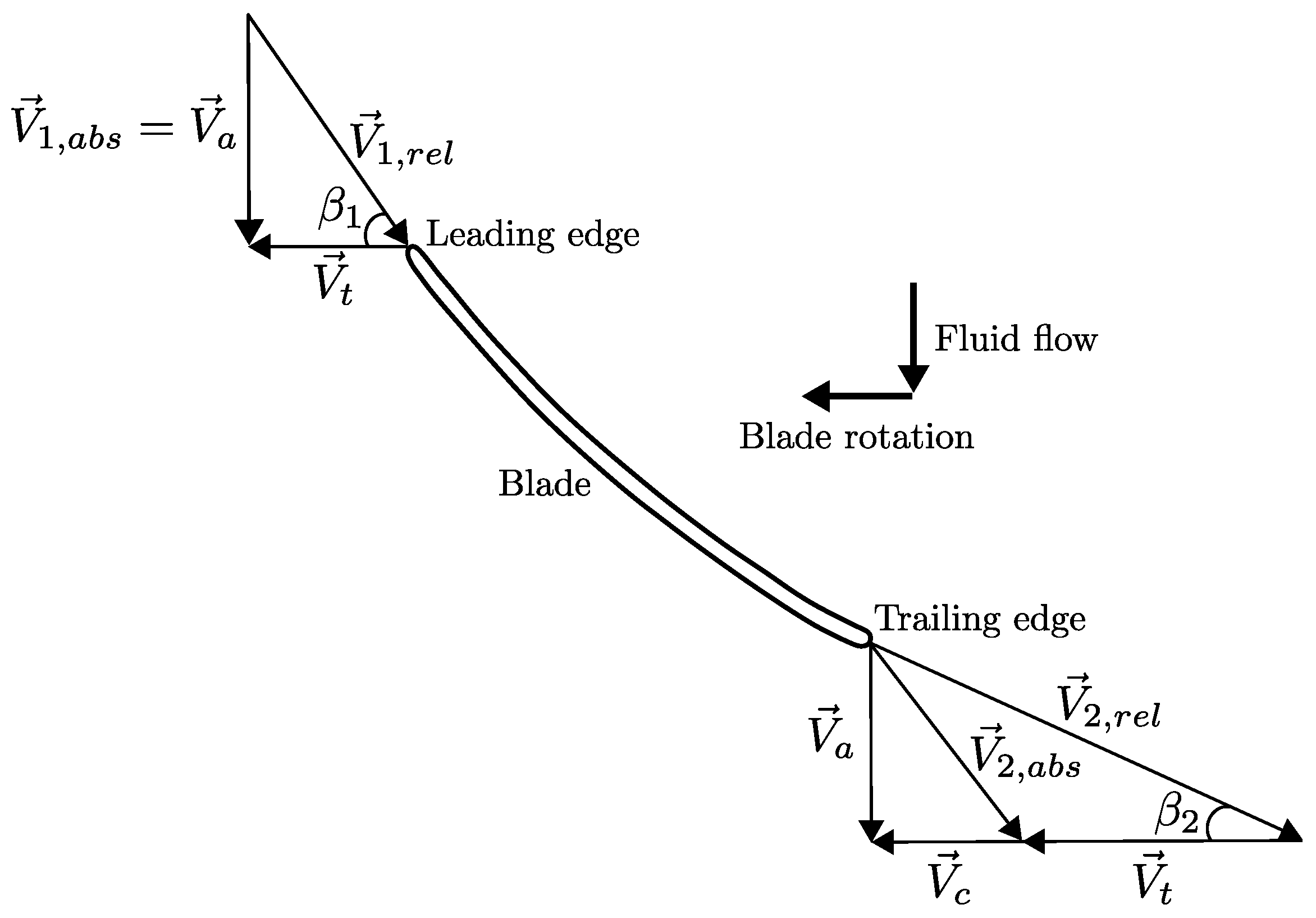
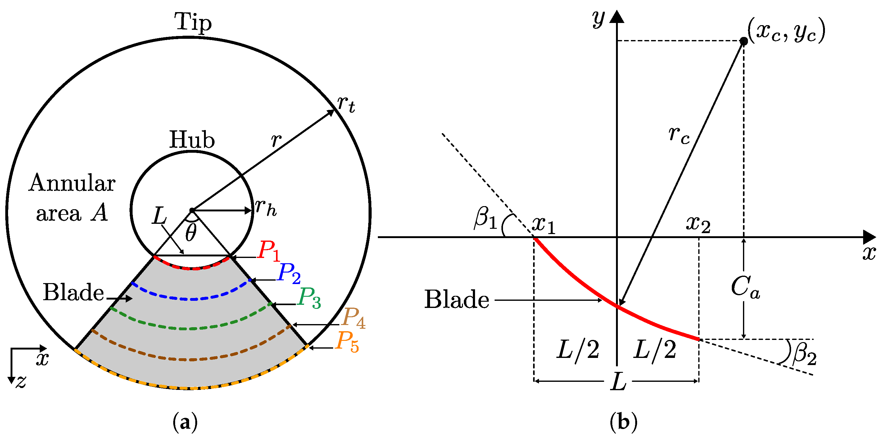
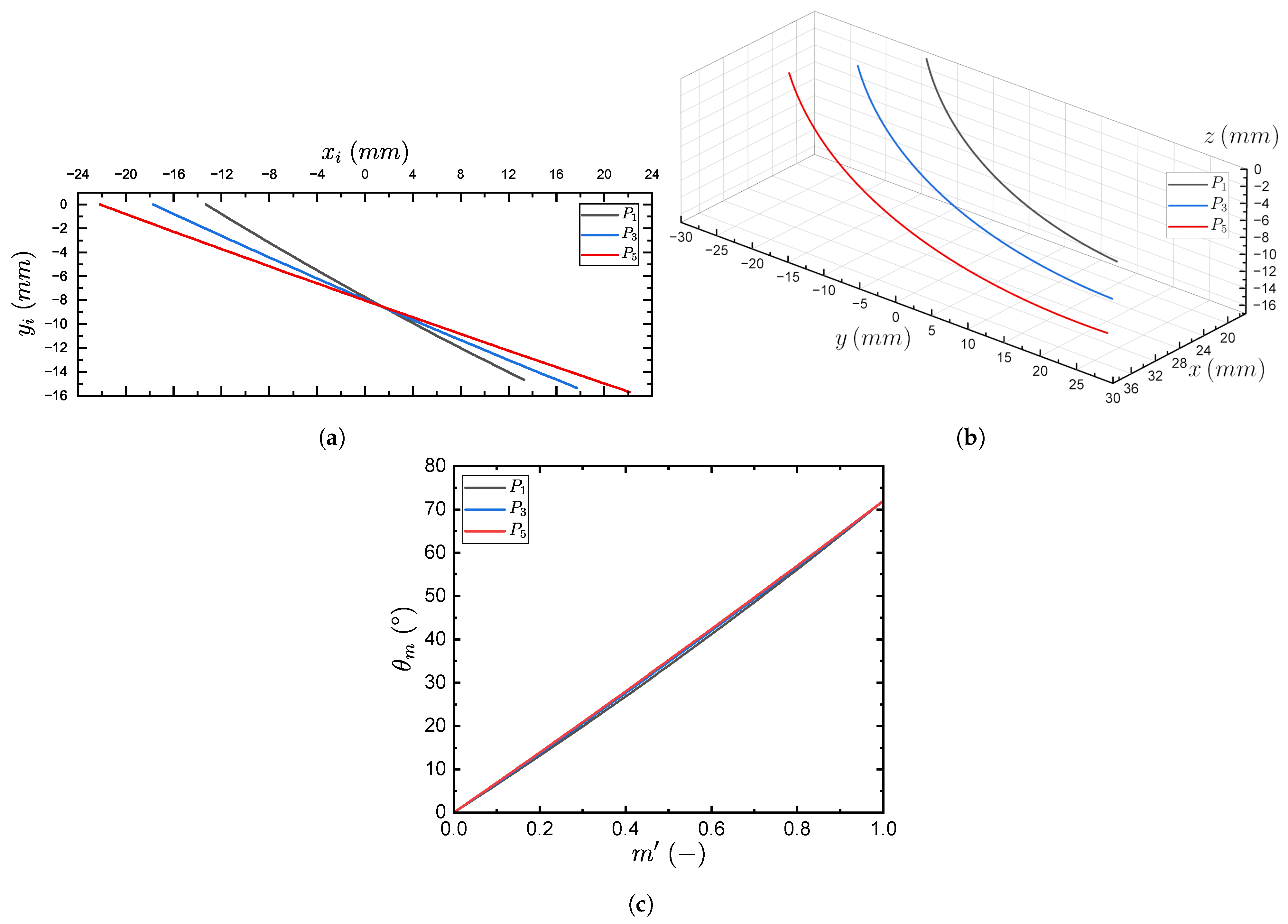
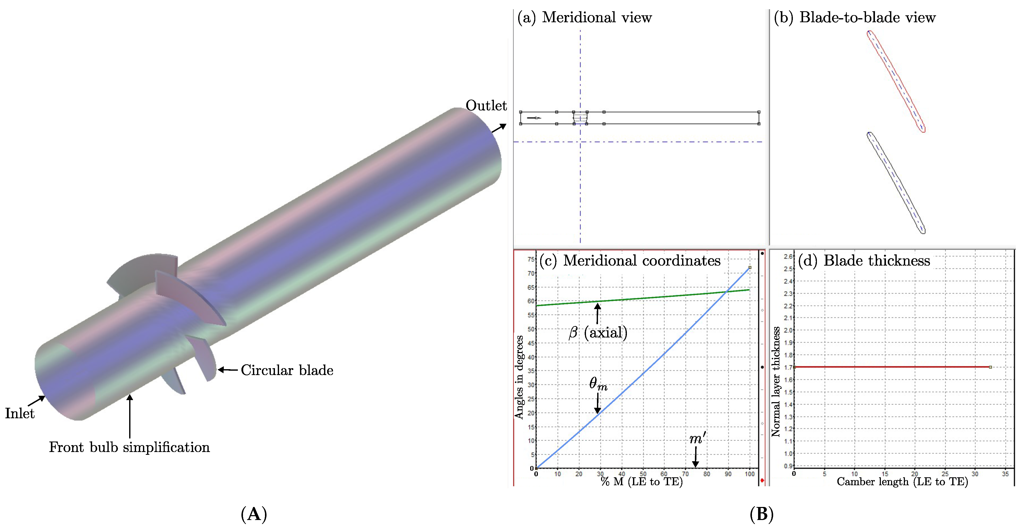
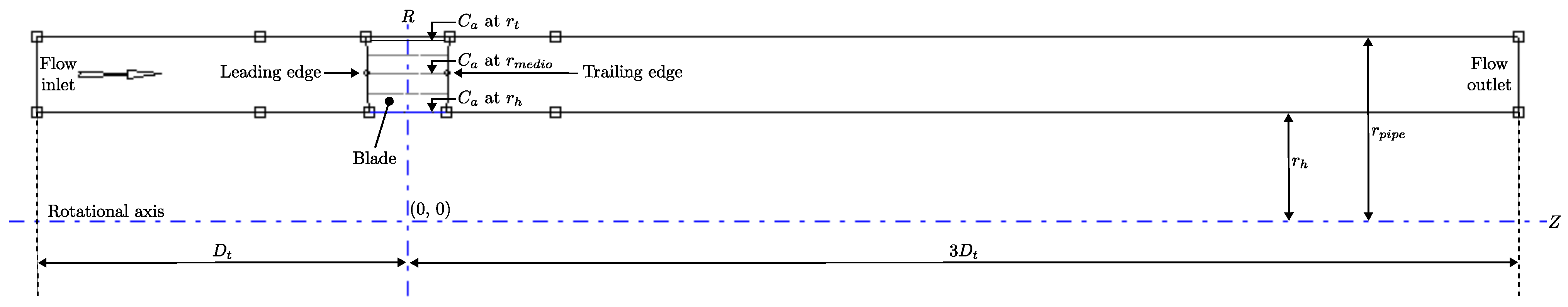
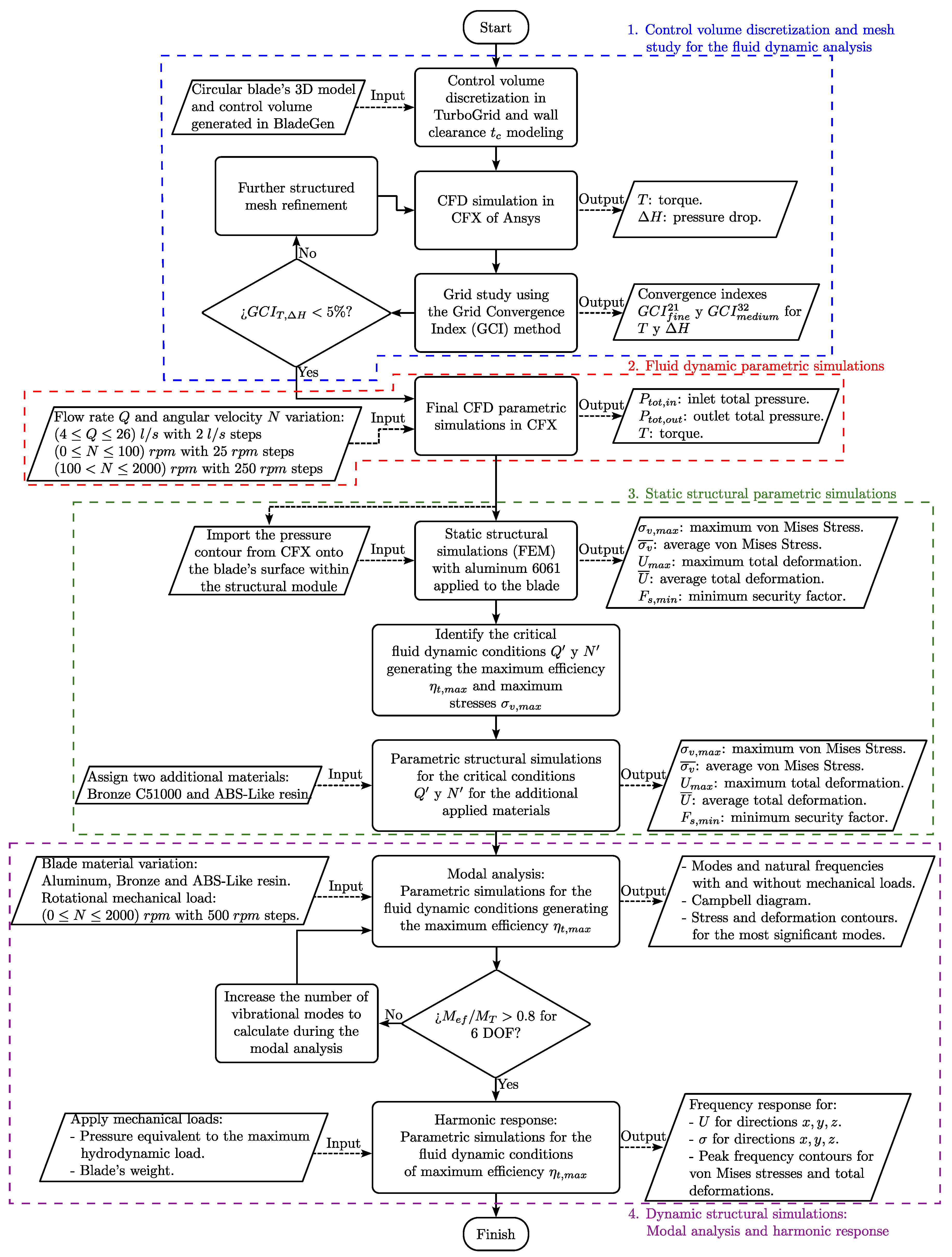

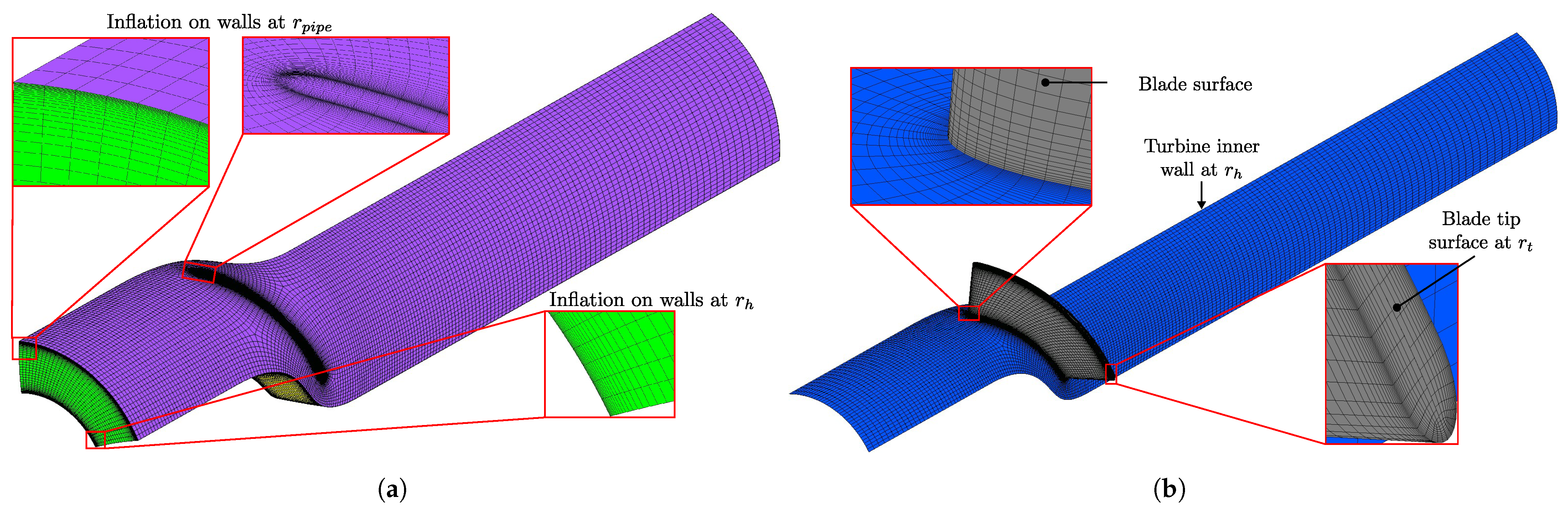

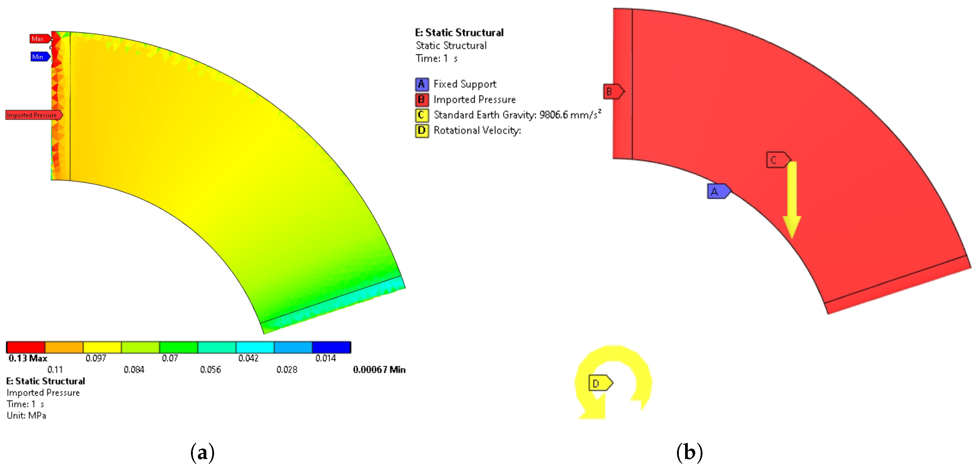
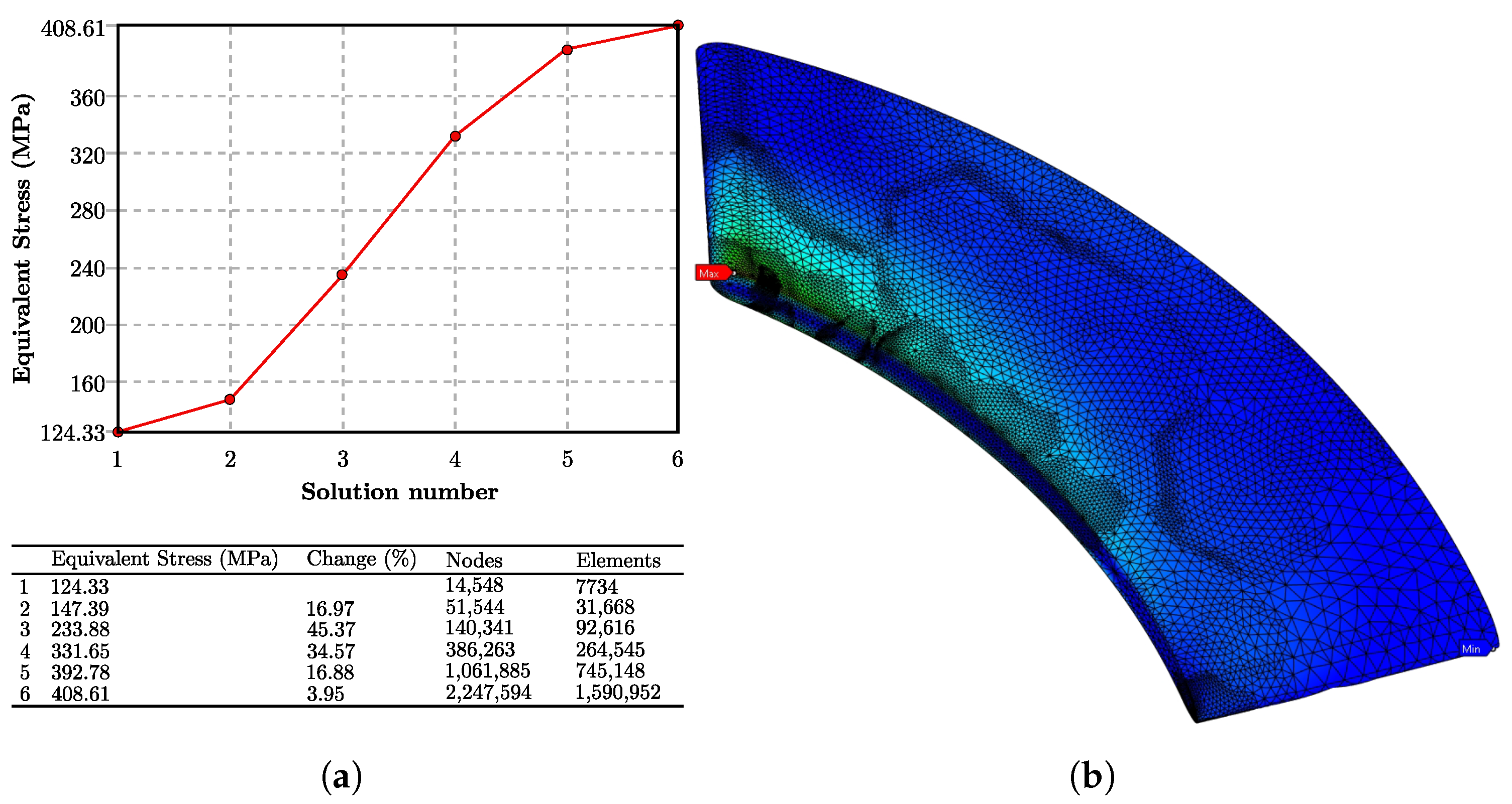
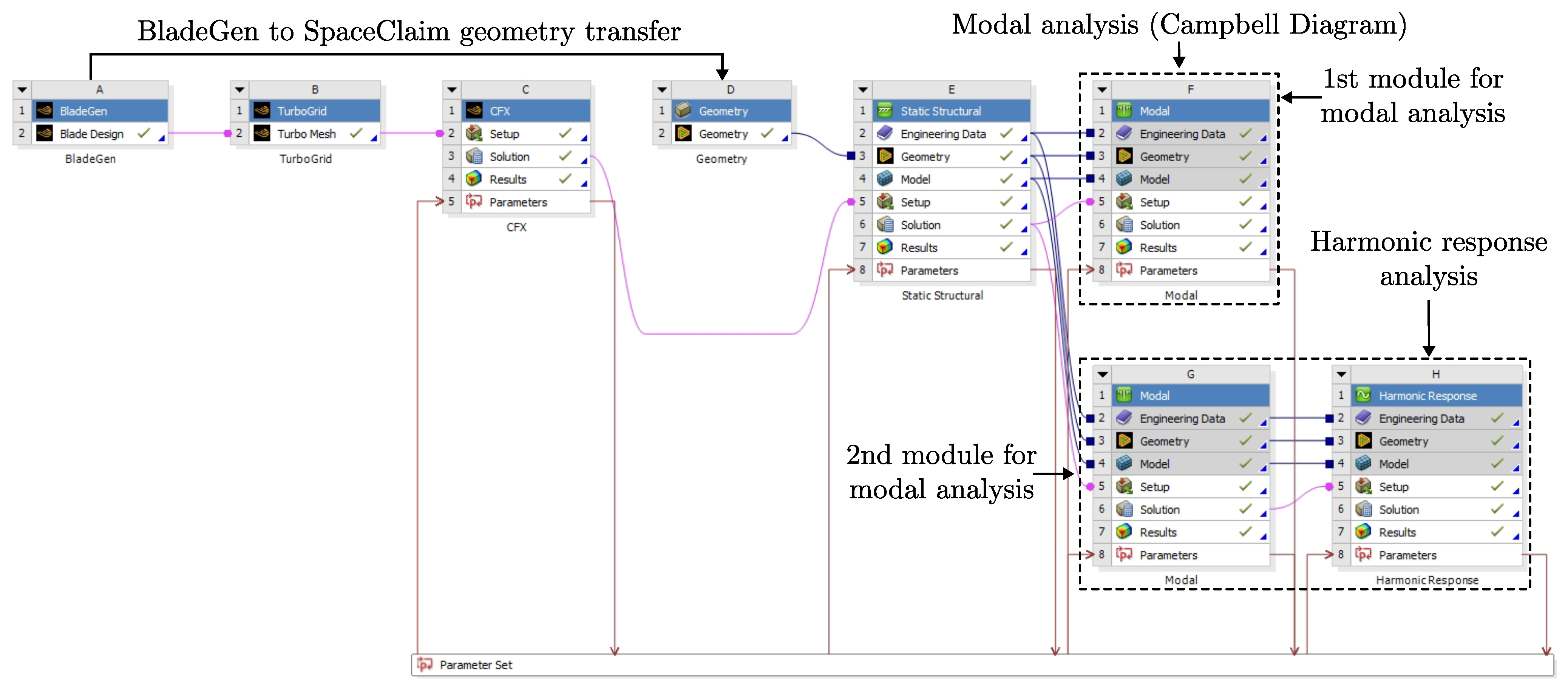
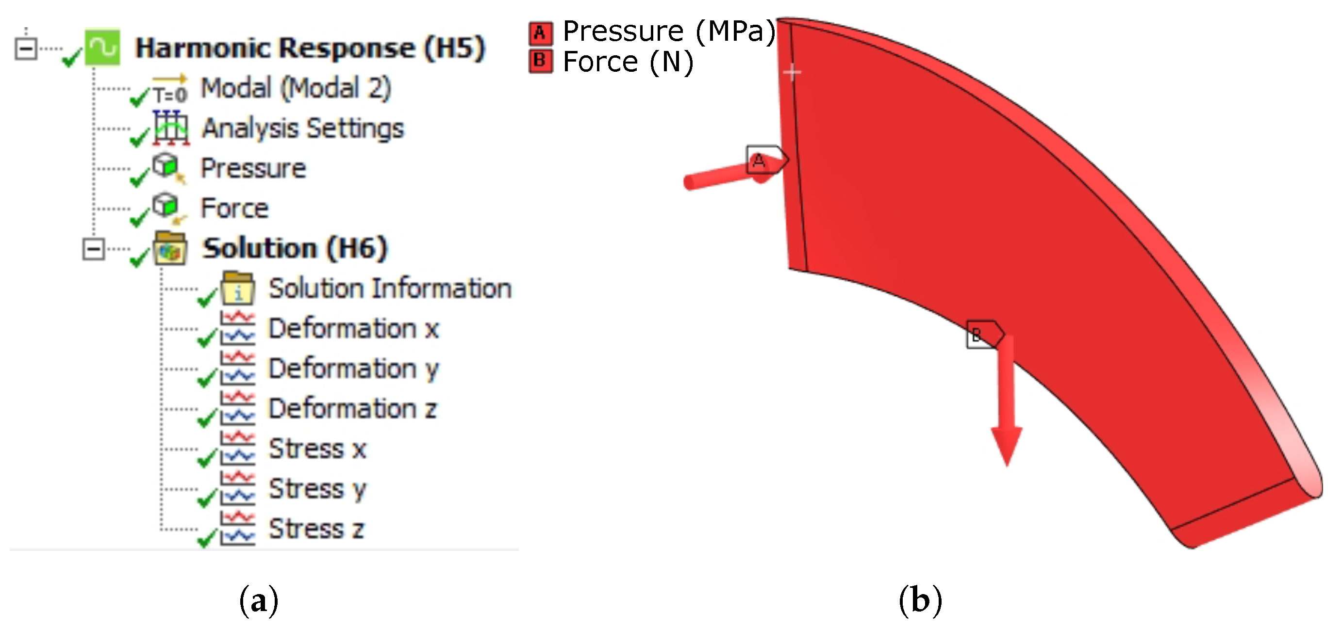

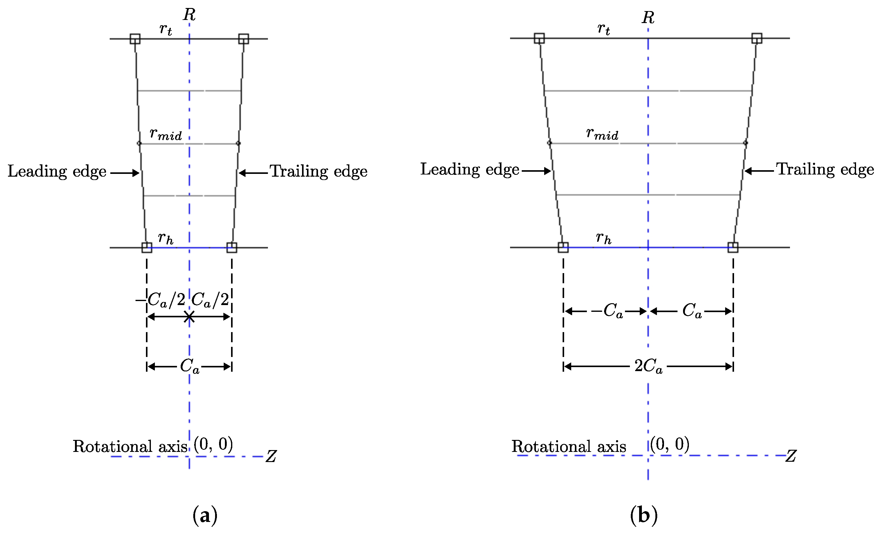
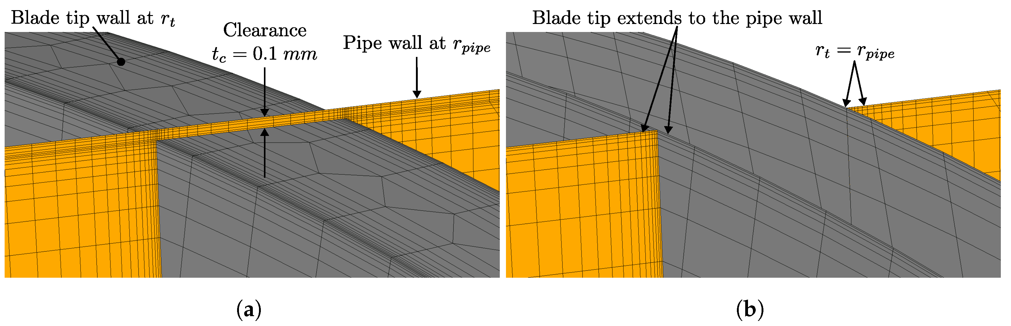

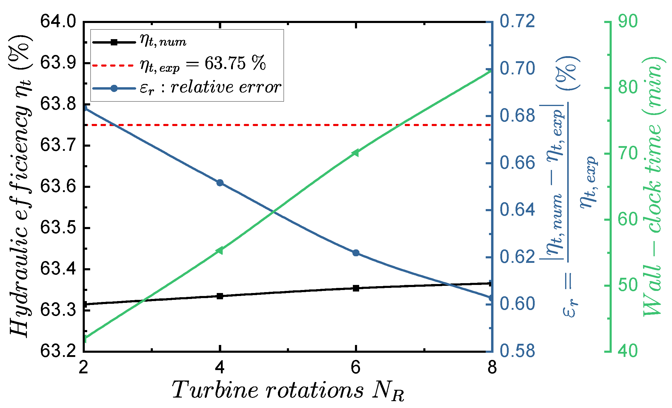
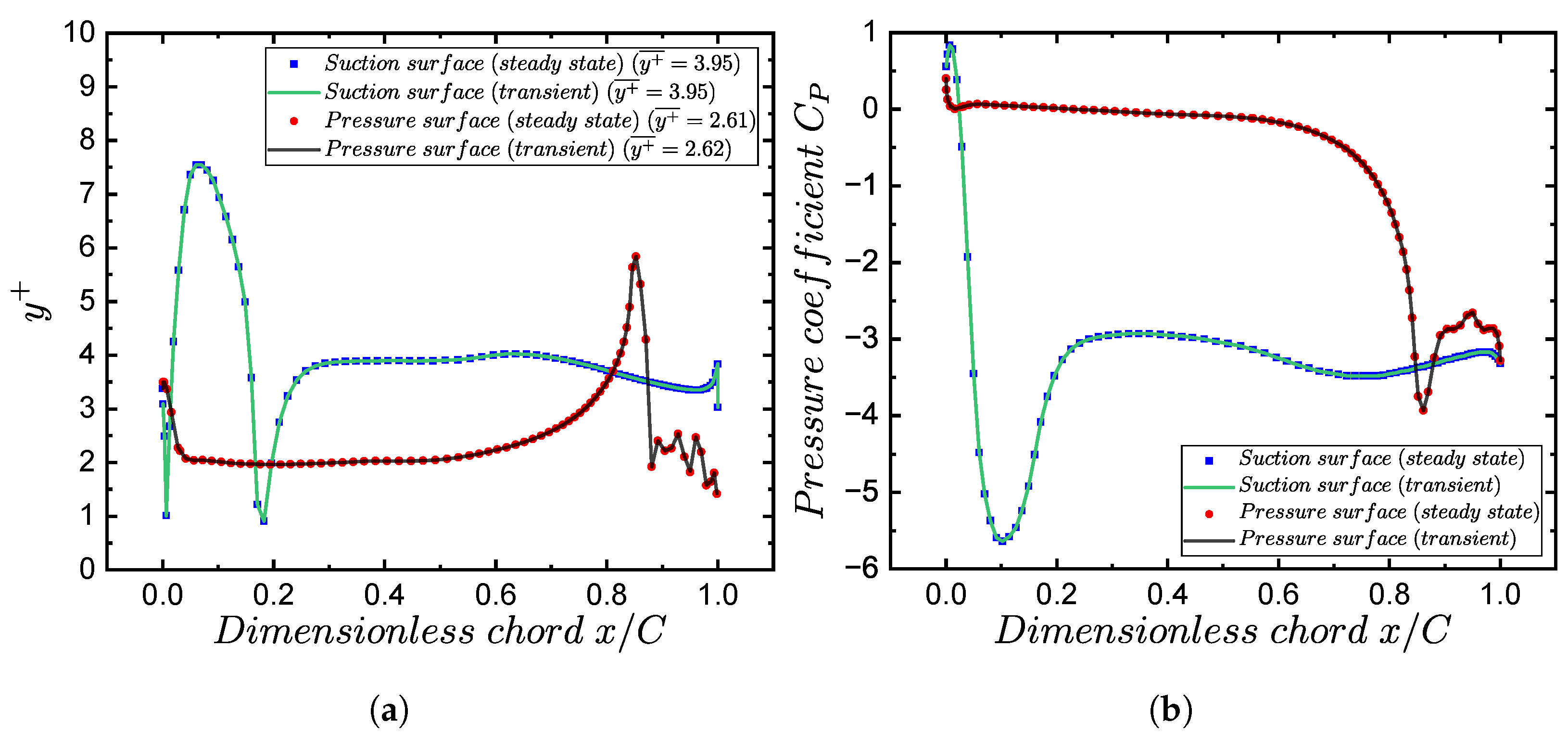
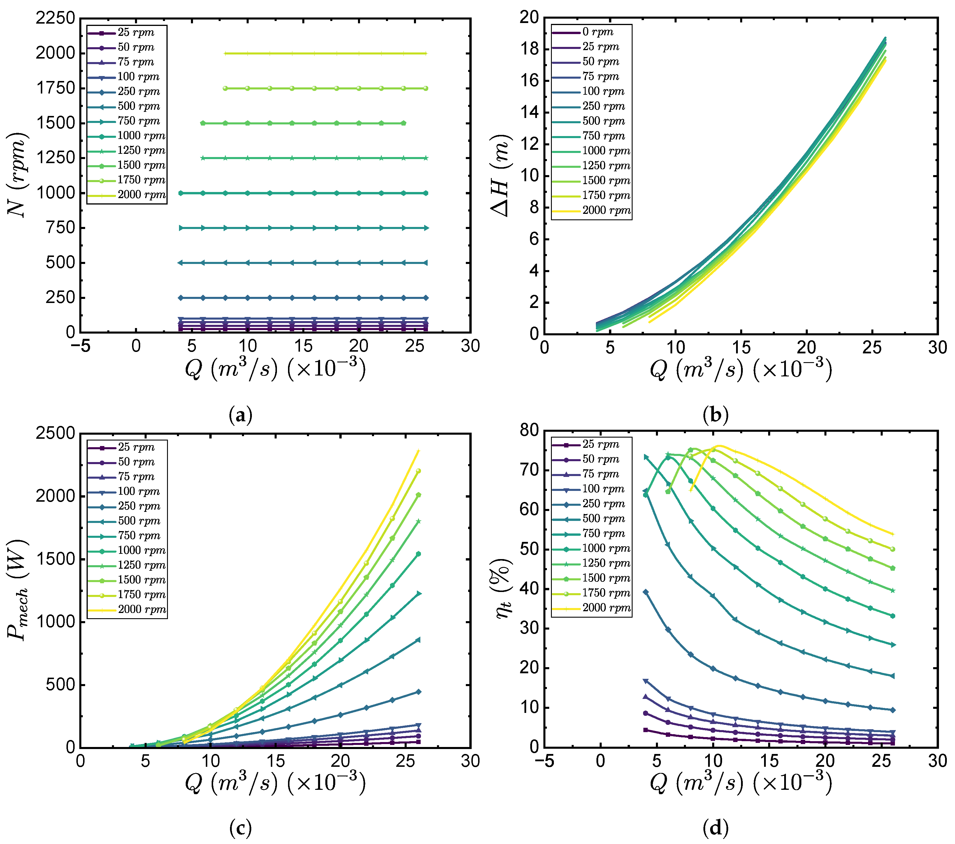
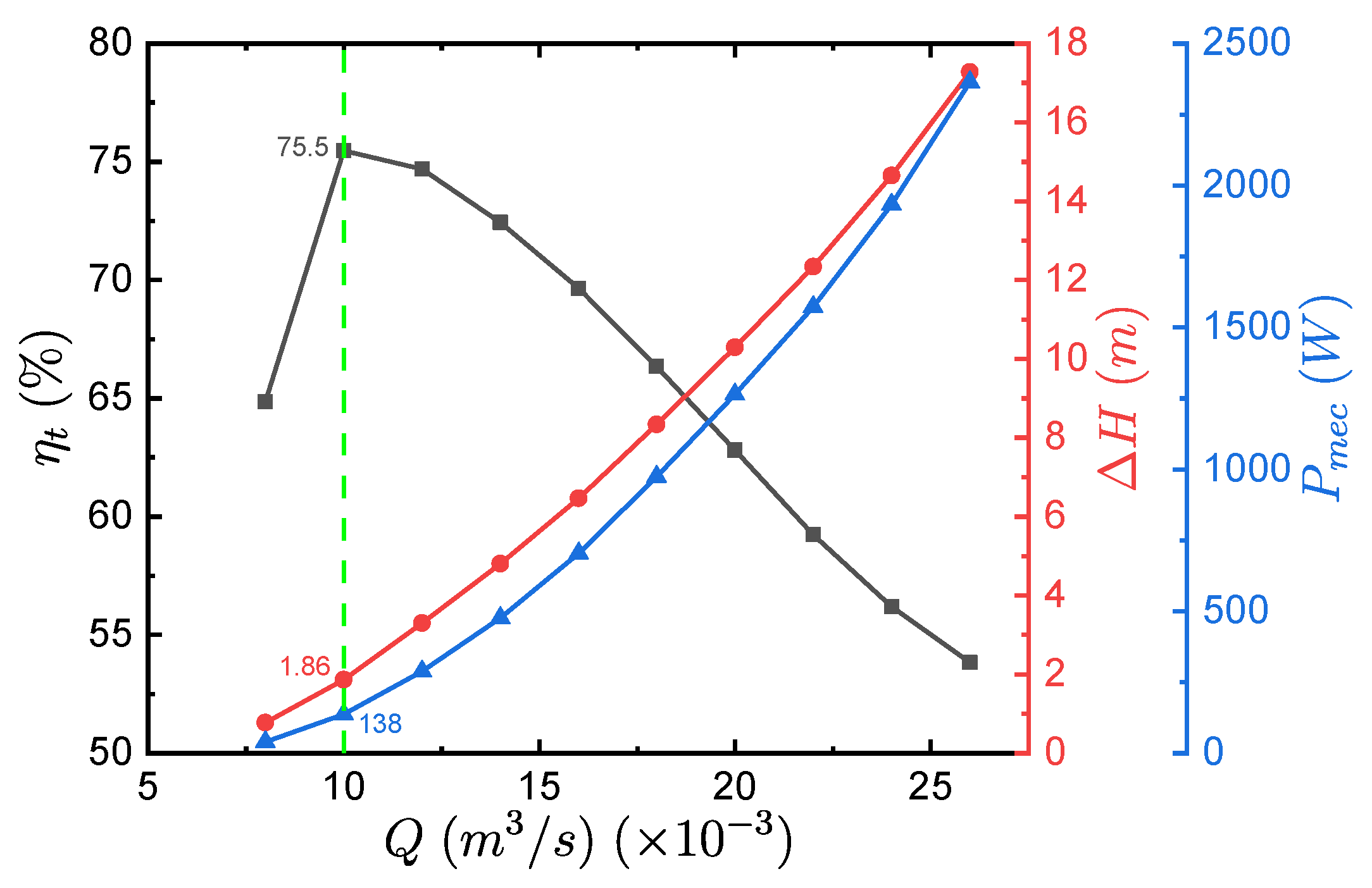
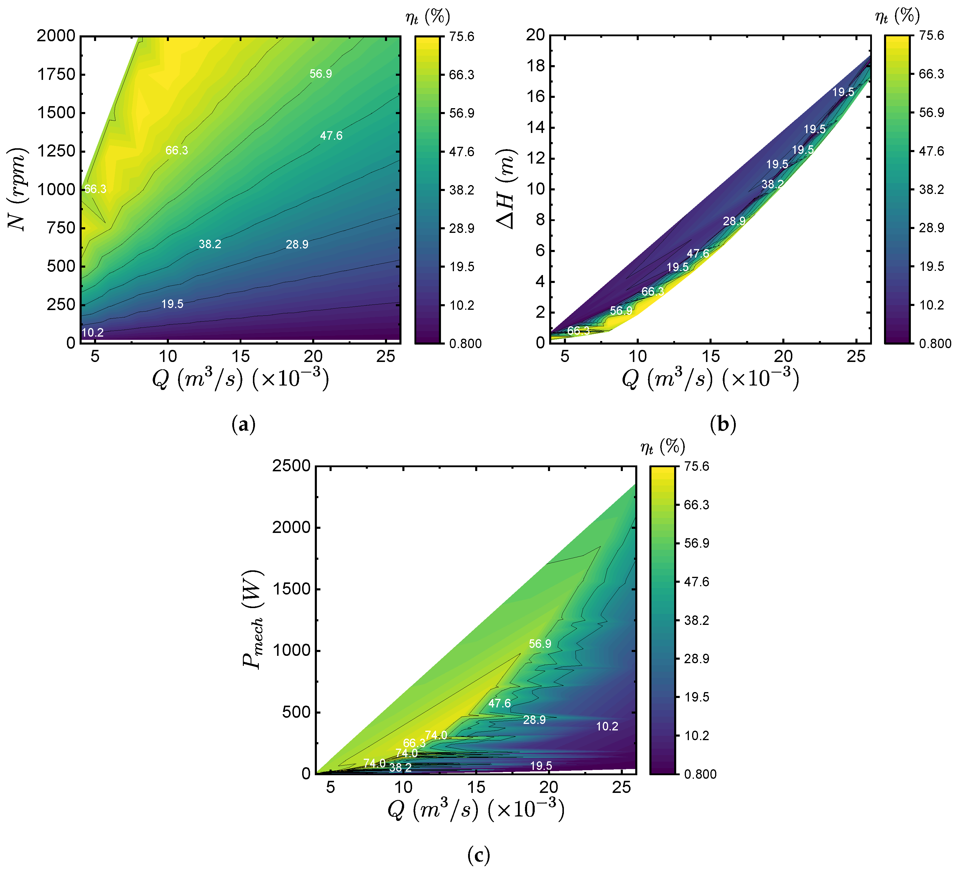
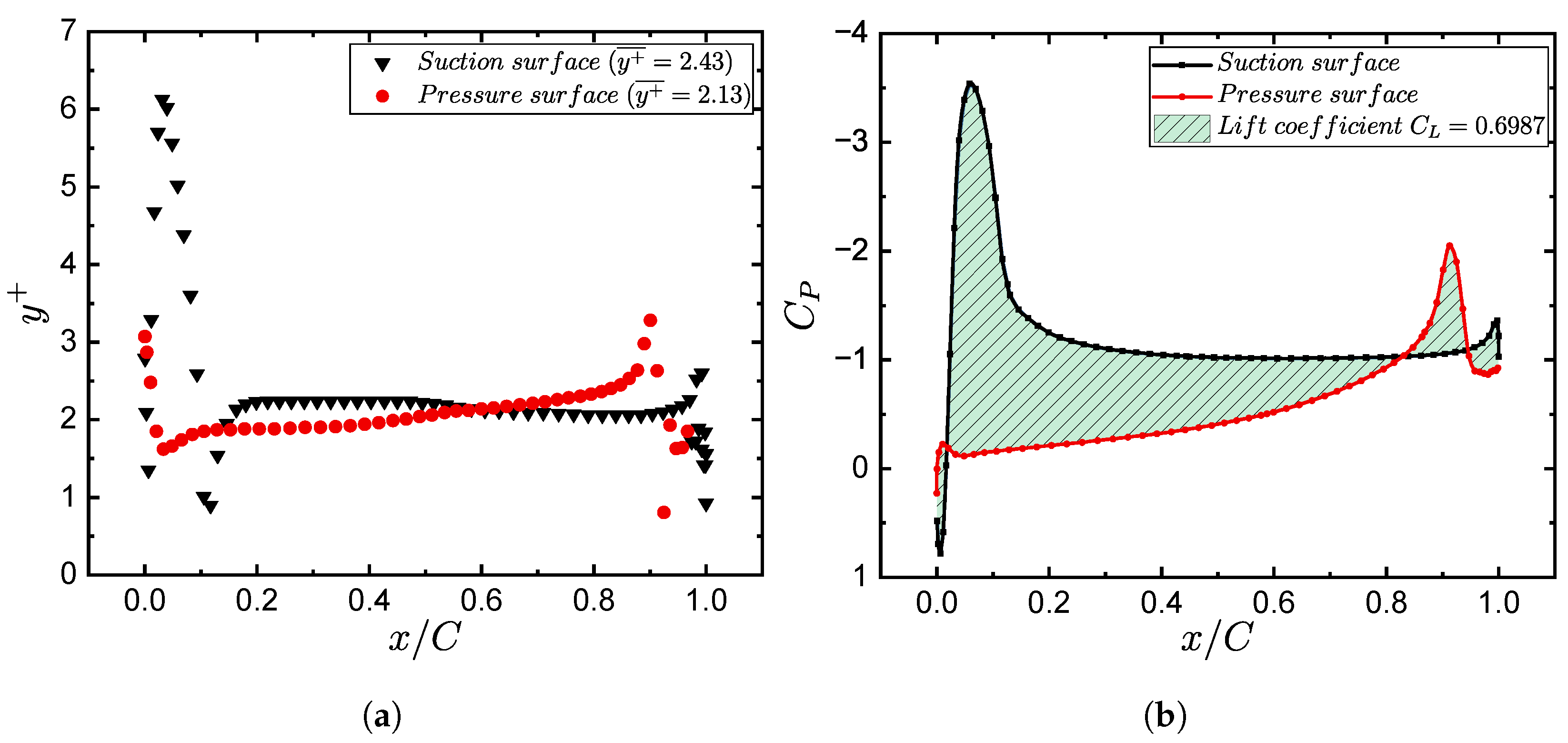

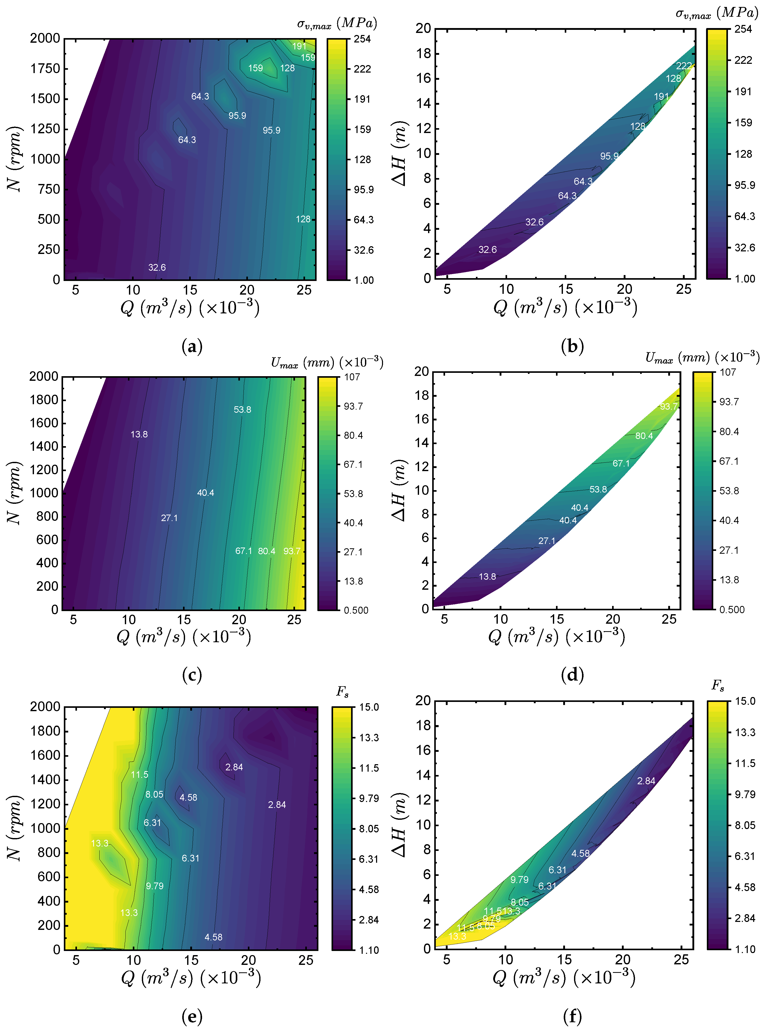
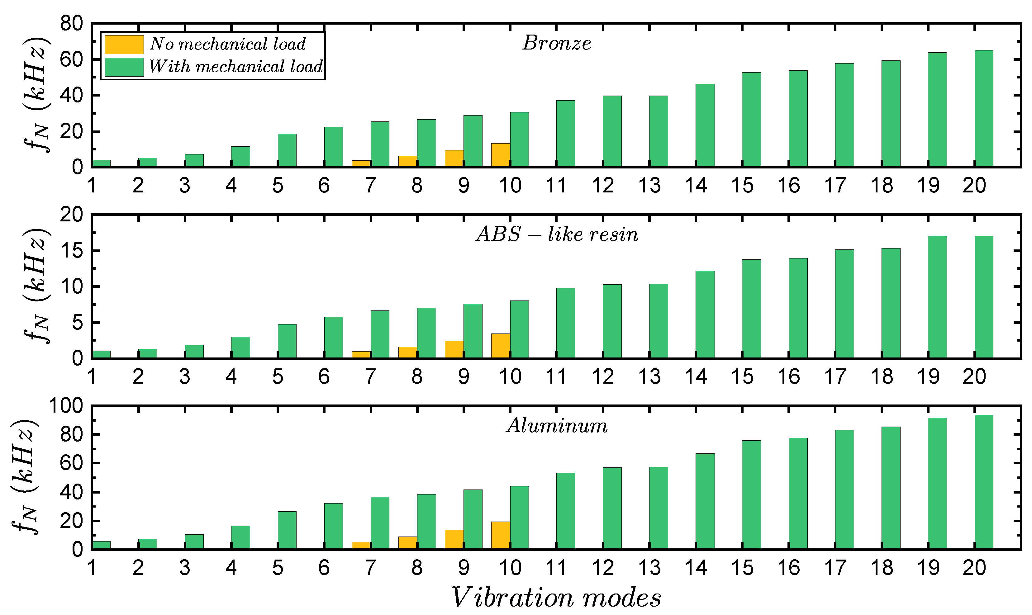
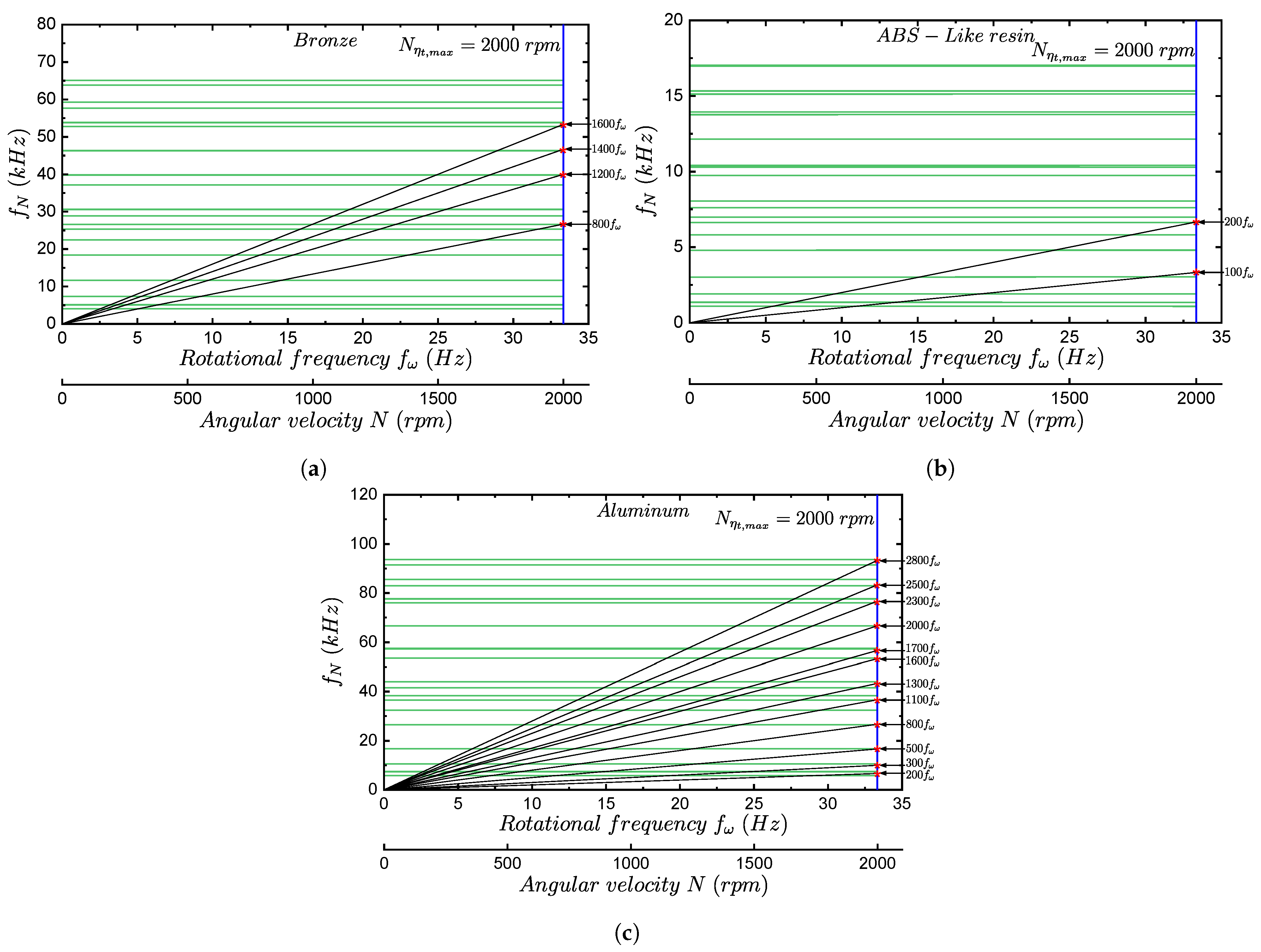
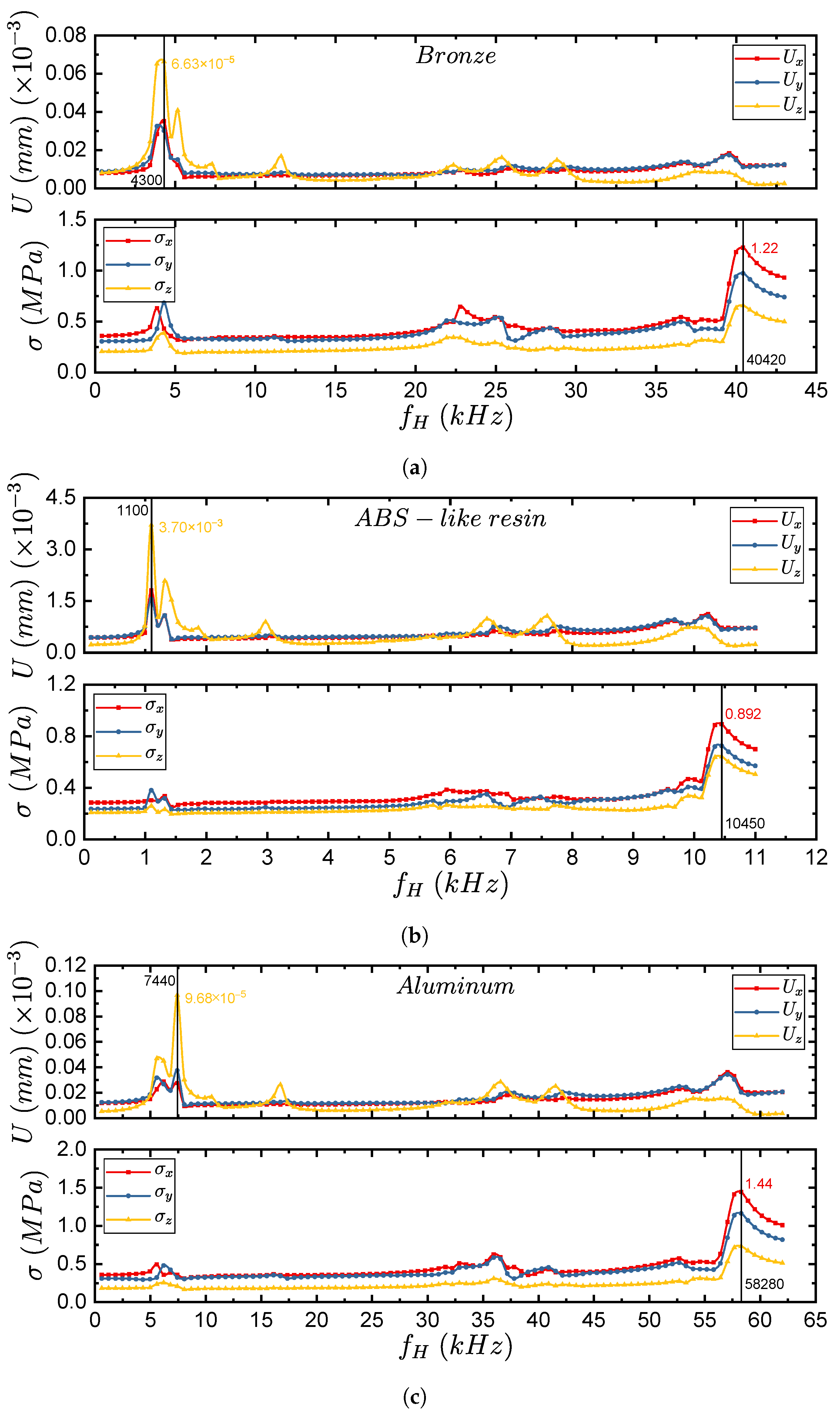
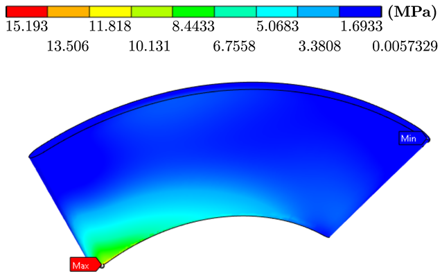
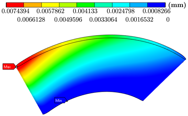
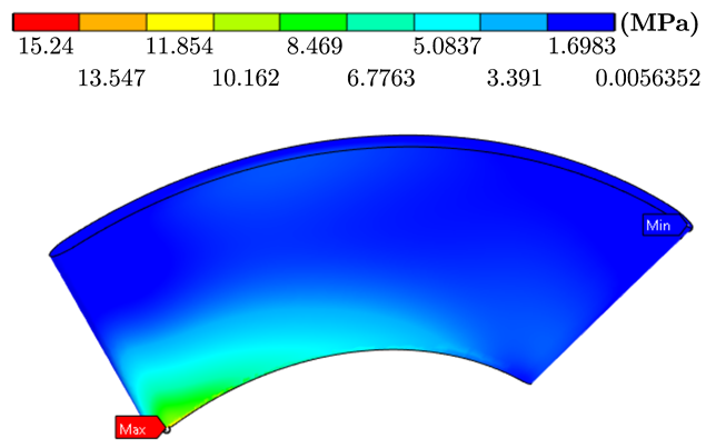
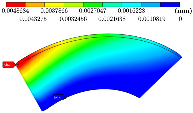
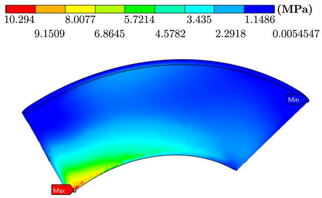
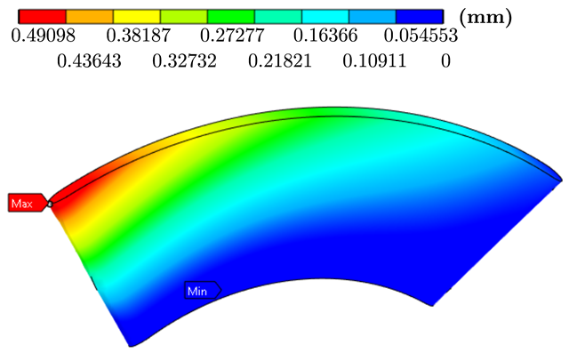
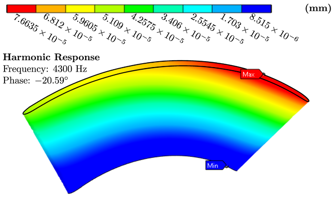
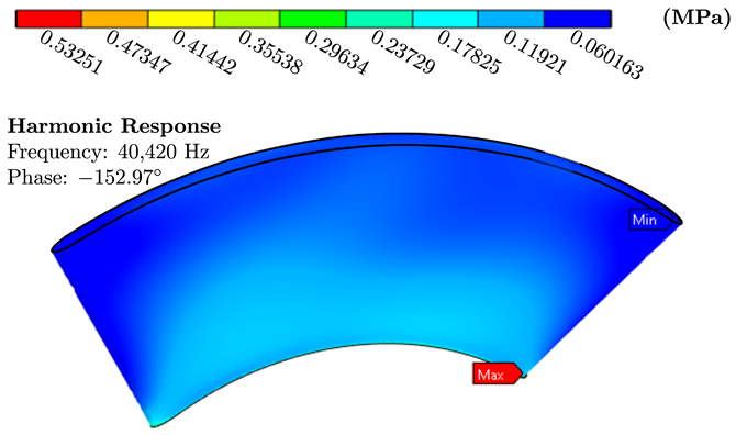
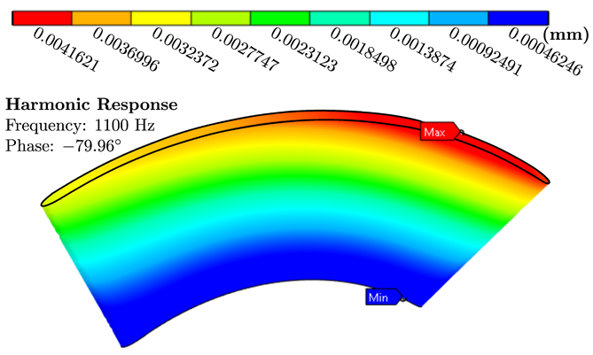
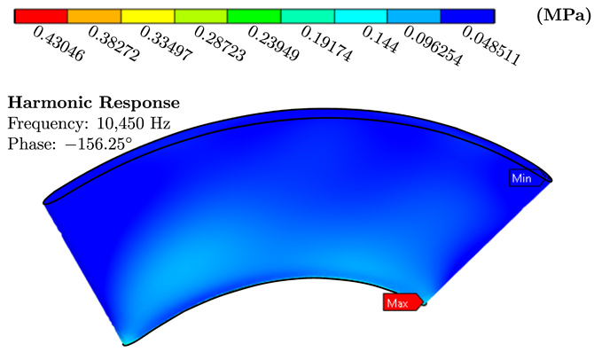
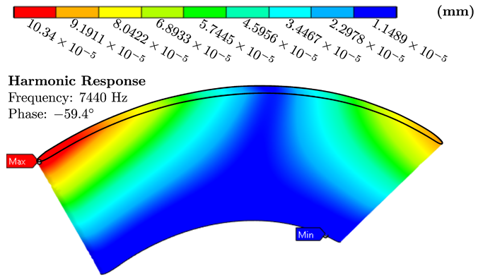
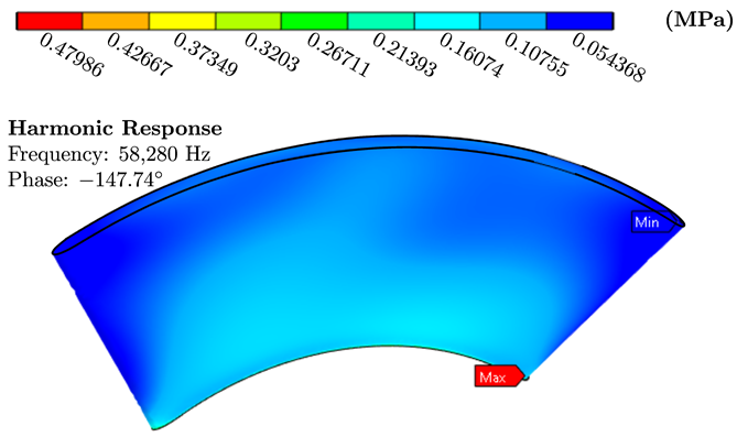
Disclaimer/Publisher’s Note: The statements, opinions and data contained in all publications are solely those of the individual author(s) and contributor(s) and not of MDPI and/or the editor(s). MDPI and/or the editor(s) disclaim responsibility for any injury to people or property resulting from any ideas, methods, instructions or products referred to in the content. |
© 2024 by the authors. Licensee MDPI, Basel, Switzerland. This article is an open access article distributed under the terms and conditions of the Creative Commons Attribution (CC BY) license (https://creativecommons.org/licenses/by/4.0/).