Abstract
Geothermal energy, being a clean energy source, has immense potential, and accurate wellbore modeling is crucial for optimizing the drilling process and ensuring safety. This paper presents a novel geothermal wellbore model based on the drift-flux approach, tested under three different temperature and pressure well conditions. The proposed model integrates the conservation equations of mass, momentum, and energy, incorporating the gas–liquid two-phase flow drift-flux model and heat transfer model. The key features include handling the heat transfer between the formation and the wellbore, addressing the slip relationship between the gas and liquid phases, and accounting for wellbore friction. The nonlinear equations are discretized using the finite difference method, and the highly nonlinear system is solved using the Newton–Raphson method. The numerical simulation, validation, and comparison with existing models demonstrate the enhanced accuracy of this model. In our tests, the model achieved a high accuracy in calculating the bottom-hole pressure and temperature, with mean relative errors (MREs) significantly lower than those of other models. For example, the MREs for the bottom-hole pressure and temperature of the Rongxi area well in Xiongan, calculated by this model, are 1.491% and 1.323%, respectively. These results offer valuable insights for optimizing drilling parameters and ensuring drilling safety. Comparisons indicate that this approach significantly outperforms others in capturing the complex dynamics of geothermal wellbores, making it a superior tool for geothermal energy development.
1. Introduction
Geothermal energy, characterized by its low carbon footprint and abundant reserves, has emerged as a highly promising renewable energy source, garnering ever-growing interest. However, as drilling depths escalate, the operational environment within geothermal wells deteriorates significantly, posing challenges for accurate parameter measurements. Consequently, therefore, employing numerical simulation for modeling geothermal wells is an excellent choice. It allows for an in-depth study of the complex subsurface environment, enabling the prediction of parameters such as the bottom-hole pressure and temperature. This predictive capability is instrumental in optimizing drilling parameters to ensure safe drilling practices.
In recent years, many researchers have conducted the modeling of geothermal wells. Bjornsson et al. have developed HOLA, a steady-state simulator for geothermal wells [1]. Tian et al. have developed a geothermal wellbore model based on the two-phase flow conservation equations. This model is used to simulate the multiphase flow inside the wellbore and the heat transfer process between the well and the formation. It is capable of handling complex drilling scenarios and achieves this functionality through input data [2]. Because steady-state geothermal wellbore models cannot accurately reflect the actual flow conditions inside the wellbore, many scholars have begun to use transient models to model geothermal wellbores. Khasani et al. used numerical simulation to establish a wellbore model to investigate the presence of CO2 gas in geothermal water and the effect of scale deposition formed in the wellbore on the flow characteristics of fluids in geothermal wells [3]. Gao et al. developed a coupled thermo-hydro-mechanical (THM) semi-numerical model for fractured reservoirs with three types of flow modes based on porous media theory, including the non-local thermal equilibrium and non-Darcy law. The study analyzed the impact of CO2 thermal properties on the heat transfer and flow inside the wellbore [4]. Saeid et al. established an efficient transient heat and fluid flow model for deep low-enthalpy geothermal systems in 2013, using finite element software for solution. In 2015, they proposed a prediction model for the lifespan of hydrothermal systems, considering a wide range of physical parameters, and similarly validated the model using the finite element method [5,6]. Brown et al. used OpenGeoSys software to evaluate the heat loss in typical low-temperature (<100 °C) single-phase geothermal systems under open-loop production conditions, with a focus on the heat loss from the bottom of the well to the wellhead [7]. The drift-flux model is commonly used to describe multiphase flow, particularly in cases of gas–liquid two-phase flow, making it especially significant for modeling the flow in geothermal wells. The drift-flux model was first proposed by Zuber and Findlay [8] in 1965. Hasan et al. used the drift-flux method to establish a robust model for two-phase flow in geothermal wells [9]. Pan et al. developed T2Well, a numerical simulator for modeling non-isothermal, multiphase, and multicomponent flow in an integrated well-reservoir system. The drift-flux model is used to solve the one-dimensional momentum equation of the mixture in the wellbore subdomain [10]. Akbar et al. developed a model that utilizes the finite element method to solve the heat and fluid flow in high-enthalpy deep geothermal wellbores. Additionally, they employed the drift-flux model to simulate the transient heat flow of a compressible, two-phase fluid traveling along the wellbore [11]. Tonkin et al. conducted a review of mathematical models for simulating geothermal wellbores, detailing the parameter definitions and differences between models. In 2023, they developed a transient geothermal wellbore simulator based on a mathematical model comprising three conservation equations (mass, momentum, and energy), and incorporating the drift-flux model established by Shi et al. [12,13,14]. Lei et al. used the drift-flux model to establish a geothermal wellbore model for controlling the two-phase flow containing CO2 in the wellbore. They proposed a robust computational method and applied this model to three production wells in the Yangba geothermal field [15]. Xu et al. developed a transient non-isothermal two-phase flow model for the dynamic simulation of multiphase flow in gas kick wellbores, with the ability to predict the temperature and pressure distribution inside the wellbore [16]. Hajidavalloo et al. developed conservation equations for the steady-state annulus and drill string, solved using the finite difference method. They analyzed the impact of temperature changes on predicting the bottom-hole pressure [17].
From the above literature, it is evident that many researchers have modeled wellbores. However, steady-state wellbore models do not account for temporal variations and, therefore, cannot simulate the dynamic changes in parameters such as temperature and pressure, nor can they adequately reflect the true flow conditions inside the wellbore. Some geothermal drilling models include the energy conservation equation, which is essential. Although some models can simulate complex multiphase flows, their descriptions of heat transfer behavior within the wellbore are insufficient, leading to less accurate predictions. Due to inaccuracies in temperature predictions, and since temperature can significantly affect the properties of the fluid in the well, pressure predictions also have inaccuracies.
This paper establishes a comprehensive transient geothermal wellbore model using the conservation equations of mass, momentum, and energy, combined with Shi et al.’s drift-flux model [14] and Hasan et al.’s heat transfer model [18]. The highly nonlinear equations in the model are discretized using the finite difference method and solved using the Newton–Raphson iteration method. The model is analyzed and validated through numerical simulation software, demonstrating promising application prospects. Additionally, comparisons with models mentioned in the literature highlight the accuracy and superiority of this model.
Compared to existing models, while the existing models consider slip phenomena, they use simplified algorithms to calculate the drift velocity in the drift-flux model. In contrast, this model takes a detailed account of slip effects, accurately reflecting the velocity differences of fluids in different flow regimes within the wellbore, thereby enhancing the model’s accuracy. This model incorporates the effects of the cement and casing on heat transfer, allowing for a more accurate simulation and prediction of wellbore temperature changes at different times and depths. It also considers the dynamic changes in system parameters (such as temperature and pressure) over time and wellbore depth, making the model’s description of wellbore behavior more realistic. This model can more precisely simulate the behavior of geothermal wellbores at different times and depths, which is of great significance for the real-time control and optimization of geothermal drilling operations, improving the efficiency and economy of geothermal wellbores.
2. Model Formulation
As shown in Figure 1, the drilling fluid exits through the drill bit nozzles and enters the wellbore annulus, carrying bottom-hole cuttings and gas–liquid mixtures back to the surface while exchanging heat with the formation in the annulus. To establish the geothermal wellbore model, the following assumptions are made:
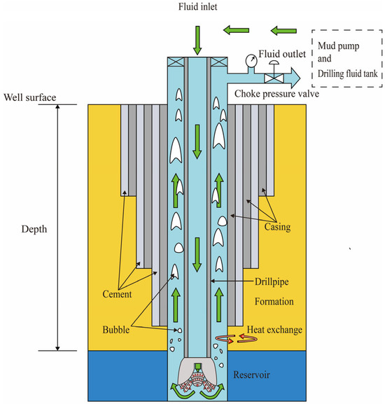
Figure 1.
Schematic of drilling circulation.
- The gas–liquid mixture flows one-dimensionally along the wellbore;
- We disregard the axial heat conduction within the wellbore;
- We disregard the impact of drill cuttings;
- We consider the impact of the casing and cement sheath on heat transfer;
- We consider the slip relationship between the gas and liquid phases.
2.1. Conservation Equations for Gas–Liquid Two-Phase Flow
In geothermal drilling, the gas–liquid two-phase flow must satisfy the conservation laws of mass, momentum, and energy. The equations are as follows:
Mass conservation equation:
ρg and ρl are the densities of the gas phase and liquid phase, respectively. vg and vl are the velocities of the gas phase and liquid phase, respectively. αg and αl are the cross-sectional gas content and cross-sectional liquid content.
Momentum conservation equation:
P is the wellbore pressure; ρm and vm are the density and velocity of the gas–liquid mixture, respectively; f is the wellbore friction coefficient; and D is the wellbore diameter.
Energy conservation equation:
eg and el are the specific internal energies of the gas and liquid phases, respectively. hTg and hTl are the total specific enthalpies, defined as the sum of the specific enthalpy, kinetic energy, and potential energy. Q represents the energy change due to the heat exchange between the formation and the wellbore. ri is the wellbore radius.
where hg and hl represent the specific enthalpies of the gas phase and liquid phase, respectively.
2.2. Constitutive Equations
Due to the large number of unknowns in these conservation equations, it is necessary to supplement them with constitutive equations. In geothermal wellbore modeling, considerations include the slip between the gas and liquid phases, friction with the wellbore wall, and heat transfer between the wellbore and the surrounding formation.
2.2.1. Mixture Equation
The relationship between the cross-sectional gas content and the mass liquid content is as follows:
The mixture density is described as:
The mass flow rate of the two-phase flow is also a crucial calculation parameter. The specific form is as follows:
2.2.2. Wellbore Friction
In geothermal drilling, the gas–liquid mixture flowing upward along the wellbore causes a significant frictional pressure drop. The expression for Ff is as follows:
The f in Equation (11) represents the wellbore friction coefficient, which can be expressed as:
where Re is the Reynolds number, and ξ is the wellbore roughness. In this paper, the roughness is assumed to be 0.00175 mm. The Reynolds number is calculated as follows:
In Equation (13), μm represents the viscosity of the gas–liquid mixture, and its expression is as follows:
2.2.3. Formation–Wellbore Heat Exchange
In geothermal drilling, there is heat transfer between the formation and the wellbore. Heat is transferred from the formation through the cement and casing into the wellbore, and the fluid inside the wellbore is transferred back to the formation through the same path. Here, we use a heat transfer equation developed by Hasan [18], applicable to any wellbore, which is expressed as follows:
kf is the formation thermal conductivity, Tei is the formation temperature unaffected by the wellbore heat transfer, and Tf is the fluid temperature inside the drill string. Radial heat exchange occurs between the formation and the wellbore fluid. When heat is transferred from the formation to the wellbore, it first passes through the cement, then the casing, and, finally, through the outer wall of the drill string into the fluid inside the drill string. Each of these parts has its own thermal resistance, so the overall heat transfer coefficient Ut can be considered as the series combination of these individual resistances, as represented by Equation (16); TD is a temperature function related to the dimensionless time td.
2.2.4. Slip Model
In the wellbore, the gas moves faster than the liquid, often resulting in slip. Since Zuber and Findlay introduced the drift-flux model, many researchers have studied various drift-flux models [19,20,21,22,23]. Currently, drift-flux correlations can be divided into three types: the first type is developed based on flow pattern characteristics [24], the second type uses smooth or weighted functions to simulate drift velocity [14], and the third type applies singular closure relationships independent of flow patterns [25]. The first type of model increases the complexity due to the diverse flow patterns at different depths and conditions during geothermal drilling. The third type assumes a single closure relationship applicable to all flow patterns, ignoring the changes in the complex flow patterns in real situations. This simplification may lead to a decreased prediction accuracy under complex flow conditions and poor performance when dealing with high-speed or low-speed modes due to its failure to consider the characteristics of different flow patterns.
The model by Shi et al. [14] exhibits a high flexibility and adaptability in handling multiphase flow. Geothermal drilling involves complex and variable flow conditions, with different depths and stages potentially involving multiple flow pattern transitions. The model by Shi et al. [14] uses smooth or weighted functions to better accommodate these changes, providing smoother computational results. Although the second type of model has a lower parameter resolution at the boundaries of the flow pattern transitions, leading to some numerical calculation accuracy reduction, this impact is relatively small in practical applications. There is inherent uncertainty in parameter measurement and actual operation in geothermal drilling, and the second type of model can generally provide accurate and stable prediction results. Additionally, the model by Shi et al. [14] has been widely used and validated in previous studies. Therefore, this study selected the second type of drift-flux model proposed by Shi et al. [14].
The two-phase velocity formula is described as:
where vm is the mixture velocity, and vd is the drift velocity.
vd is a crucial parameter in the drift-flux model, and, in wellbore models, many factors can affect its magnitude. Liu et al. [26] recently pointed out that the Taylor bubble velocity increases with the inclination angle and decreases with increasing liquid viscosity. This means that drift velocity decreases as the yield point of viscosity increases. Therefore, in the drift velocity calculation model in this paper, the inclination angle factor is considered, while the impact of viscosity is not explicitly accounted for. This is because, in geothermal drilling, the high bottom-hole temperature requires the drilling fluid to be maintained in a high-speed circulating state to ensure effective cuttings removal and drill bit cooling. Additionally, the drilling fluid and two-phase flow are in a turbulent state. Under turbulent conditions, inertial forces dominate, making the effect of rheology on overall flow characteristics minimal [27]. The expression for vd is as follows:
In this slip model, m(θ) is a function of the wellbore inclination angle, C0 is the profile coefficient, K is a function of the cross-sectional gas content, and vc is the characteristic velocity.
In a gas–water dominated system, the expression for m(θ) is:
Here, the improved K by Pan et al. [21] based on Shi’s model [14] is used.
where Ku is the “critical Kutateladze number” related to the pipe diameter.
The expression for the characteristic velocity vc is:
The formula for the profile parameter C0 is:
This equation ensures that C0 has a constant value during bubble flow or slug flow, and equals 1 during annular mist flow. The expression for the parameter γ is:
Fv is a constant used to adjust the sensitivity of C0 to velocity. vsgf is the critical velocity value that prevents the liquid film from falling back with the gas flow.
After experiments conducted by Shi et al. [14], it was found that, in the gas–water system, the optimal parameter A is equal to 0, α1 = 0.06, and α2 = 0.21. Therefore, the calculated value of C0 is equal to 1.
2.3. Supplementary Equations
2.3.1. Density Equation
The gas and liquid phase densities in this paper are selected based on the model proposed by Fjelde et al. [28]. The specific form is as follows:
In the formula, ag and al represent the speed of sound in the gas phase and the liquid phase, respectively. Their values are 316 m/s and 1000 m/s.
2.3.2. Viscosity Equation
The gas viscosity calculation model used in this paper is based on the model proposed by Lee et al. [29]. The specific form is as follows:
In these equations, M represents the molecular weight.
3. Numerical Methods
In geothermal drilling simulations, selecting the appropriate numerical method is crucial for accurately simulating the complex interactions of the multiphase flow, heat transfer, and pressure changes. The finite difference method (FDM) is a common numerical analysis technique used to solve differential equations. It discretizes the differential equations in a specified region, transforming continuous problems into discrete ones [30,31]. Lou et al. [32]. combined the energy equation in finite difference form with the AUSMV numerical format of the drift-flux model, creating a transient non-isothermal wellbore multiphase flow model with broad applicability. Liu et al. [33]. developed an improved gas migration velocity model under shut-in conditions and embedded the drift-flux model into the new gas migration velocity model using the AUSMDV hybrid numerical format.
While the advection upstream splitting method (AUSM+) performs well in capturing sharp discontinuities and handling compressible flows, the finite difference method (FDM) has unique advantages in geothermal well simulations. The FDM is widely favored for its numerical stability and implementation simplicity, and is particularly suitable for handling structured grids and smoothly varying flow characteristics. In geothermal drilling simulations, the primary focus is on the gradual changes in temperature and pressure profiles along the wellbore. The FDM provides a robust framework, ensuring the stability and accuracy of the numerical solution without the need for the complex flux splitting techniques required by the AUSM+. At the same time, the FDM offers greater flexibility in implementing various boundary conditions, allowing for more a accurate representation of the thermal and hydraulic interactions at the wellbore boundaries. The AUSM+ is relatively complex in handling boundary conditions, particularly in the coupling of multiphase flow and heat transfer.
While the FDM is highly efficient in handling linear equations, it may encounter convergence issues when dealing with nonlinear equations. Therefore, combining the FDM with the Newton–Raphson iteration method significantly improves this aspect, enhancing the convergence speed and accuracy, especially exhibiting a rapid quadratic convergence near the true solution. Below are the model solution steps in this paper:
- Initialize the pressure and temperature: First, set the initial pressure and temperature values, then divide the wellbore into grids.
- Calculate the velocity and phase fractions: Use the mass conservation equation and momentum conservation equation to determine the fluid velocities and phase fractions. This step involves calculating the movement properties of the fluids within the wellbore.
- Calculate the temperature: Apply the energy conservation equation to compute the temperature, considering the heat conduction within the wellbore fluids.
- Newton–Raphson iteration: Since the discretized equations form a nonlinear system, use the Newton–Raphson iteration method. Based on the current values of velocity, phase fractions, temperature, and pressure, compute the Jacobian matrix and iterate to solve the nonlinear equations.
- Error and convergence check: Compare the calculated residuals with the convergence criteria. If the error is less than the threshold of 10−6, the solution is considered converged, and the loop can end.
- Update the solution and continue the loop: If the solution has not converged, update the velocity, phase fractions, temperature, and pressure values based on the Newton–Raphson iteration results and error assessment. Then, return to step 1 to continue the iteration process.
- Advance to the next time step: Once the simulation converges, proceed to the next time step and continue simulating the wellbore conditions at the next moment.
3.1. Discretization of Equations
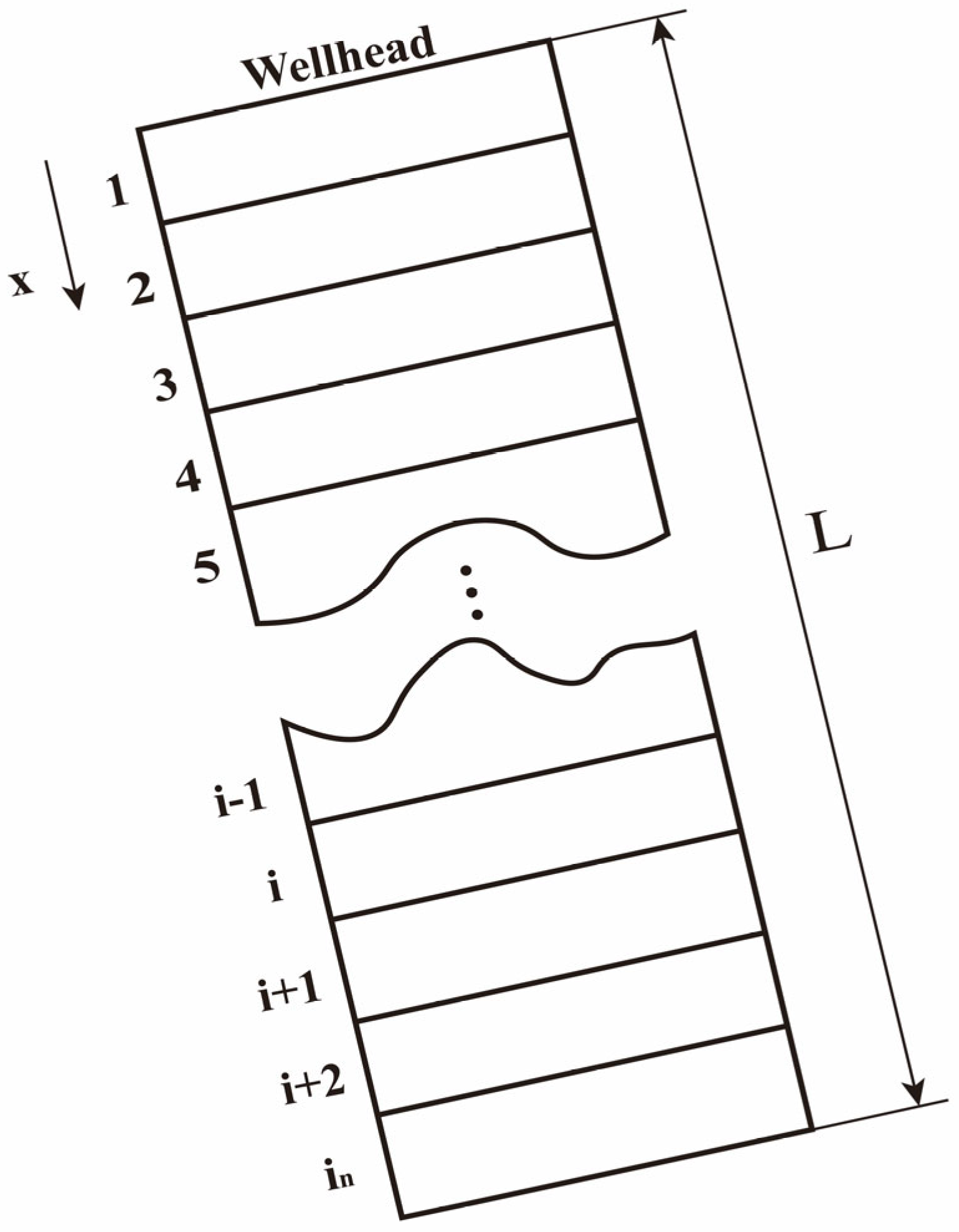
3.1.1. Grid Division
To accurately simulate the geothermal wellbore model, the wellbore is divided into in discrete grid cells along its length, with a total length of L and an increment of Δx for each segment (see Figure 2). Detailed calculations of pressure, temperature, velocity, and phase fractions are performed from the initial grid point at the wellhead, iterating down to the bottom of the well.
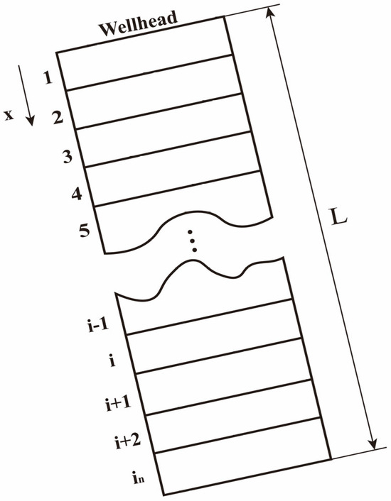
Figure 2.
Wellbore grid division.
3.1.2. Mass Conservation Equation
The mass conservation equation is discretized in time and space using a forward difference scheme, given as follows:
3.1.3. Momentum Conservation Equation
The momentum conservation equation is discretized as follows:
3.1.4. Energy Conservation Equation
The energy conservation equation is discretized as follows:
3.2. Boundary Conditions
The boundary conditions in the geothermal wellbore model are crucial for the model’s accuracy and need to be precisely defined.
3.2.1. At the Wellhead
The temperature at the wellhead is determined by the temperature of the drilling fluid at the wellhead, and is thus expressed as:
The pressure at the wellhead is the sum of the dynamic pressure and the backpressure; thus, the expression for the pressure at the wellhead is:
3.2.2. At the Bottom Hole
Due to the significant influence of the formation temperature at the bottom of the wellbore, the temperature inside the wellbore is expressed as Equation (34), where ΔT represents the temperature loss, determined according to Fourier’s law of heat conduction, and ΔZ represents the distance between the wellbore and the formation:
Assume the bottom-hole pressure is equal to the formation pressure:
3.3. Newton–Raphson Iteration
After discretization, the conservation equations remain nonlinear. Therefore, the Newton–Raphson method is used for an iterative solution. The Newton–Raphson method has many advantages, such as efficiency and fast convergence, and it has shown good application effects in wellbore modeling [34,35,36].
Assuming the solution vector is:
The residual vector F is calculated from the conservation equations. The mass conservation equation, momentum conservation equation, and energy conservation equation are represented as F1, F2, and F3, respectively. Additionally, the equations from the drift-flux model and the heat transfer model are used as auxiliary residual equations F4 and F5.
The increment Δu is obtained by multiplying the inverse of the Jacobian matrix by the residual vector.
The iterative formula for solving the solution vector in conjunction with the auxiliary equations mentioned earlier is given by Equation (45):
4. Model Verification and Analysis
To validate the effectiveness of the model, three sets of comparative experiments were conducted using geothermal wells from different locations. The first set involved a geothermal well in the Rongxi area of Xiongan, China. Rongxi is an important part of the Xiongan New Area Rongcheng group. To meet winter heating needs, geothermal resources are scientifically and reasonably developed in compliance with laws and regulations. This set of data provides a practical application scenario to test the model’s performance during the drilling process. The specific parameters of this geothermal well are listed in Table 1.

Table 1.
Parameters of a geothermal well in the Rongxi area.
The second set of experiments used the SNLG87-29 well data provided by Garg et al. [37]. This well is a highly representative slimhole geothermal well. The slimhole SNLG87-29 well is completed with a 4.5-inch casing (102 mm internal diameter) to a depth of 159.7 m, with an open hole (99 mm internal diameter) completion used below this depth. The pressure and temperature curve data were recorded on 5 August 1993. This experimental data provides a historical comparison basis for the model, helping to verify its accuracy and reliability in handling and predicting data over different time periods.
The third set of experiments utilized data from the No. 6 well at point D in northwest Iran, as mentioned in the article by Zolfagharroshan et al. [38]. This well is located in the Sabalan region southeast of Meshkinshahr, Iran, and was drilled in 1974 for the construction of a geothermal power plant. The data from this well not only demonstrate the model’s applicability under different geographical and geological conditions but also highlight its potential in energy development applications.
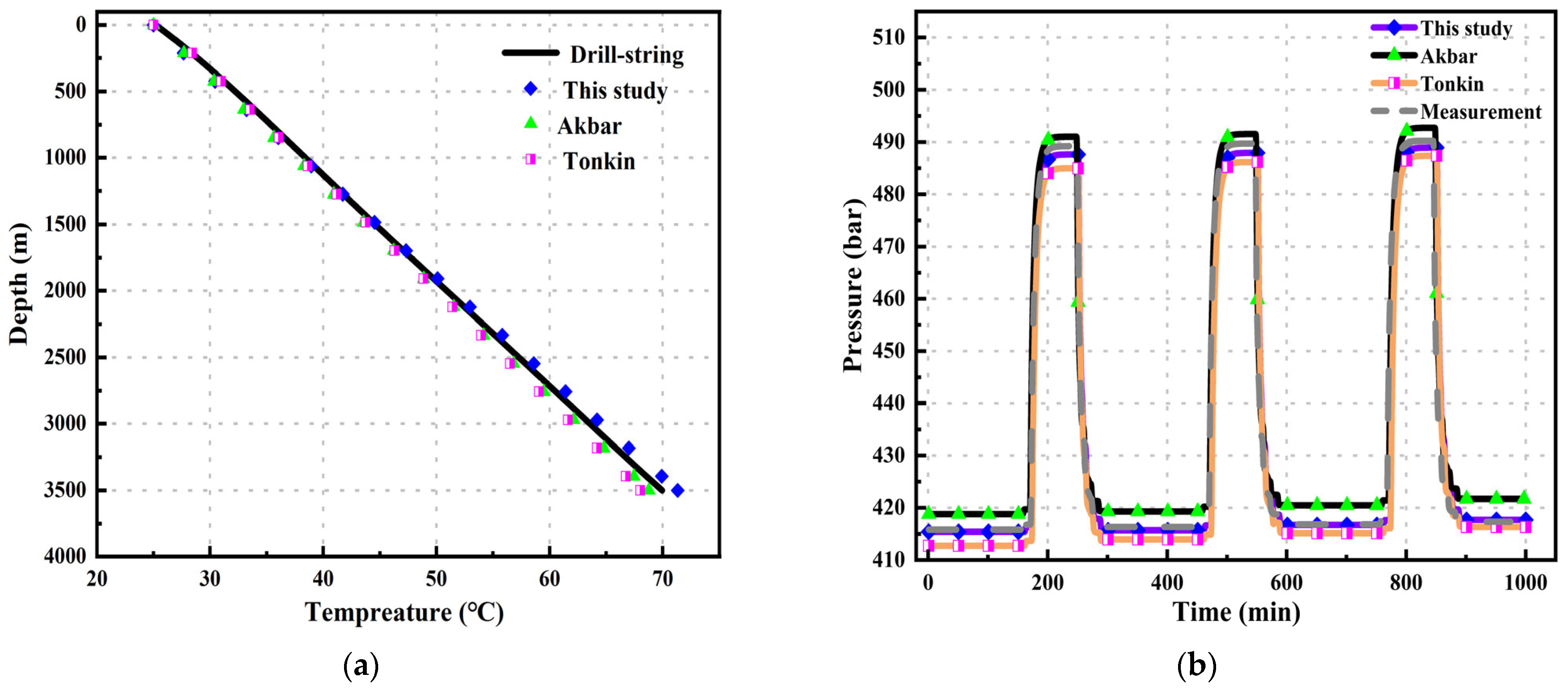
Based on the data in the table, calculations using the model produced results as shown in Figure 3. Figure 3a presents the measured temperature data inside the drill pipe. After comparing and validating with the models by Akbar et al. and Tonkin et al., the results are as follows: All three wellbore models provide accurate temperature calculations. The mean relative error (MRE) for this model is 1.323%. For Akbar’s model, the MRE is 1.999%, and, for Tonkin et al.’s model, the errors are 1.78%. This indicates that the temperature calculation model in this study is relatively accurate.
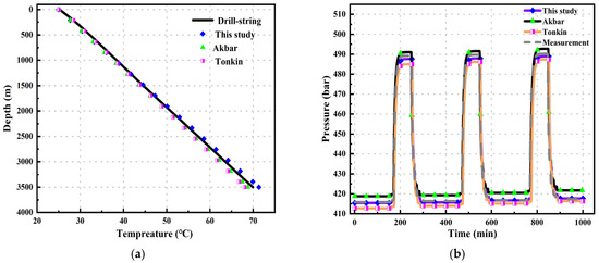
Figure 3.
Xiongan Rongxi area well: (a) temperature results performance of different models; and (b) pressure results over time for different models.
Figure 3b shows the trend of bottom-hole pressure over time. As the drilling depth increases over time, the bottom-hole pressure increases. However, due to various uncertainties in the formation, the bottom-hole pressure may suddenly change, necessitating adjustments to the surface backpressure to control the bottom-hole pressure. The figure shows that the model in this study provides a good fit during the stable drilling phase, outperforming the other two models. When the bottom-hole pressure suddenly changes, the MRE in the calculated results is 1.491%, which is smaller than the MRE calculated by the other two models.
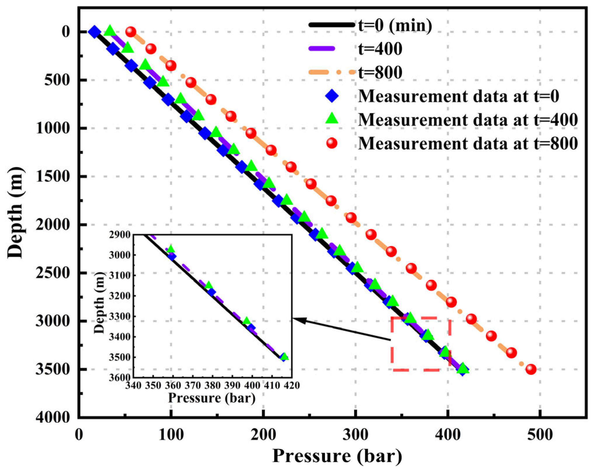
To clearly and intuitively demonstrate the pressure calculation results of various geothermal wellbore models, pressure–depth curves were plotted at different time points: t = 0, 400, and 800.
Figure 4 shows that both the wellhead pressure and the bottom-hole pressure increase with time. The pressure–depth curves calculated by this model at different time points match well with the actual measured data. The mean relative errors (MREs) at the three different time points are 1.254%, 1.254%, and 1.339, respectively.
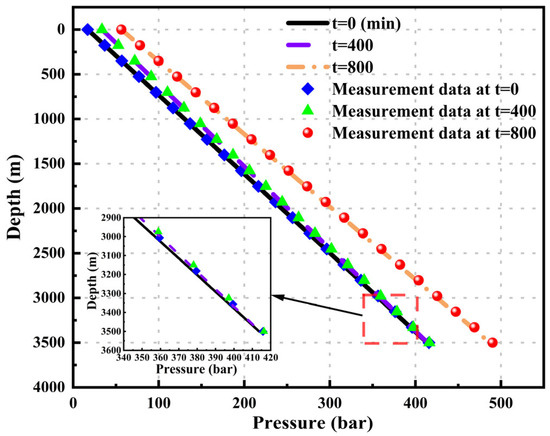
Figure 4.
Comparison of the pressure–depth curves calculated by this model with the measured results.
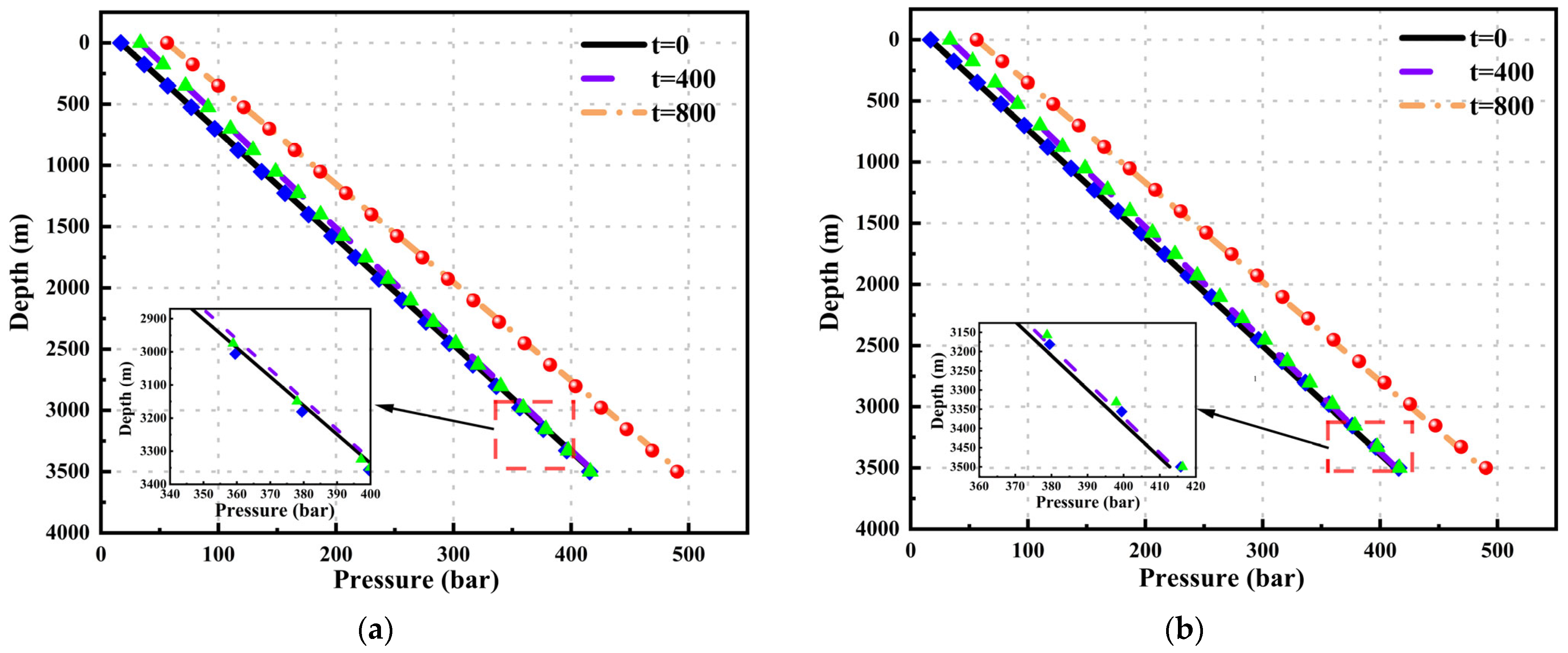
Figure 5 shows the pressure results calculated by Akbar’s model and Tonkin’s model. The mean relative errors (MREs) calculated by Akbar’s model at different time points are 2.036%, 2.035%, and 2.025%, while the MREs calculated by Tonkin’s model at different time points are 2.037%, 2.029%, and 2.029%.
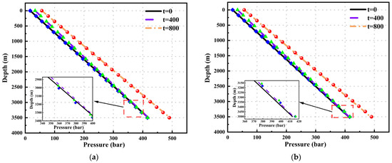
Figure 5.
The pressure results calculated at different time points as a function of depth: (a) Akbar’s model; and (b) Tonkin’s model.
The specific parameters of the SNLG87-29 well are listed in Table 2.
Table 2.
Parameters of SNLG87-29 well.
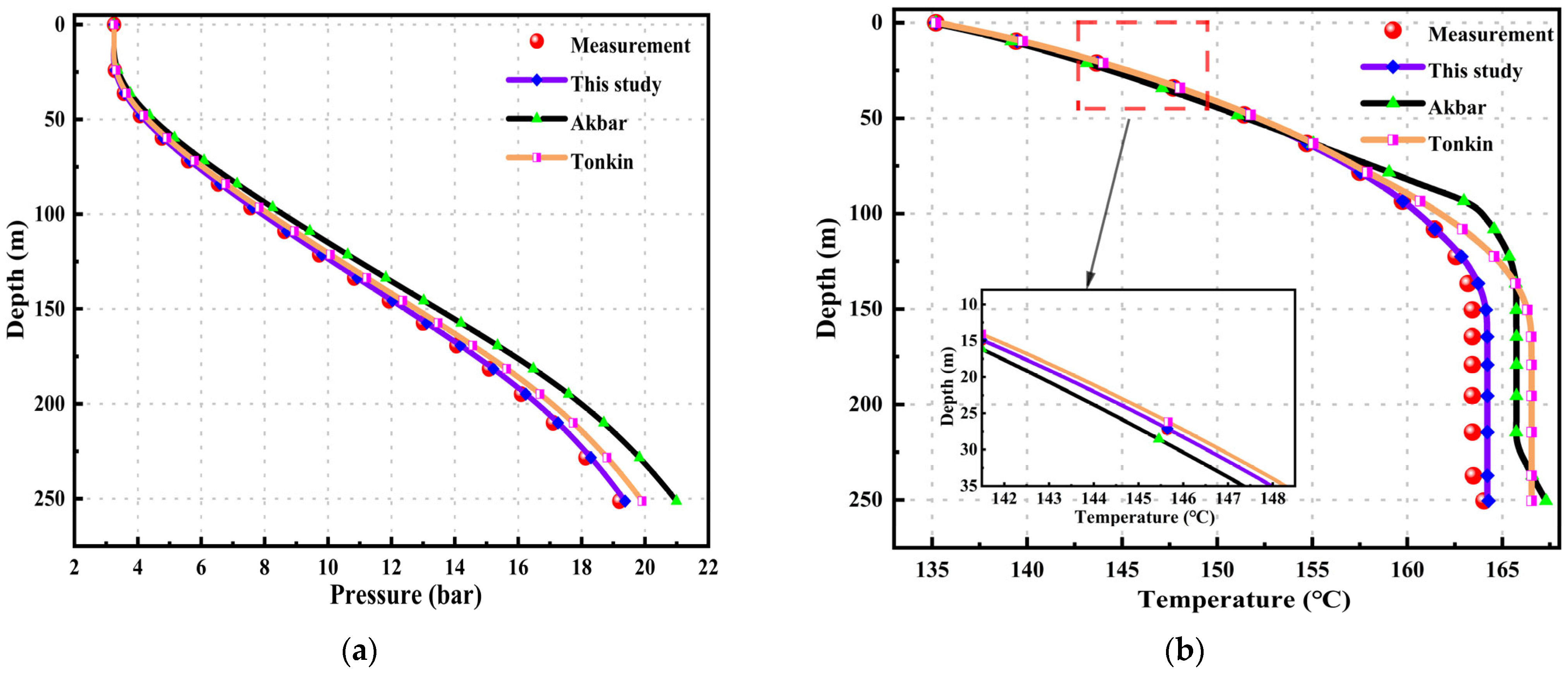
Based on the existing parameters and some initial parameter assumptions, calculations were performed for this geothermal well. The results are shown in Figure 6.

Figure 6.
SNLG87-29 well: (a) pressure vs. depth curve; and (b) temperature vs. depth curve.
Figure 6a illustrates the pressure variation with depth. It can be clearly observed that the measured data align well with the model presented in this study, with an MRE of 1.824%. Given the shallow depth and low pressure of the well, all three models show good fitting results. The MRE for Akbar’s model is 4.624%, and, for Tonkin’s model, it is 3.213%.
Figure 6b depicts the temperature variation with depth. In the initial 75 m, all three models fit the measured data well. However, as the temperature gradient changes, the temperature variation with depth decreases. Akbar’s model retains the trend of the original data curve but has a higher MRE, which is 2.203%. The model presented in this study shows a similar trend to Tonkin’s model, but with an MRE of 1.209%, which is lower than Tonkin’s.
This indicates that the model presented in this study performs well even in high-temperature, low-pressure wells.
Zolfagharroshan et al. [38] mentioned the detailed parameters of Well No. 6, listed in Table 3.
Table 3.
Parameters of No. 6 well.
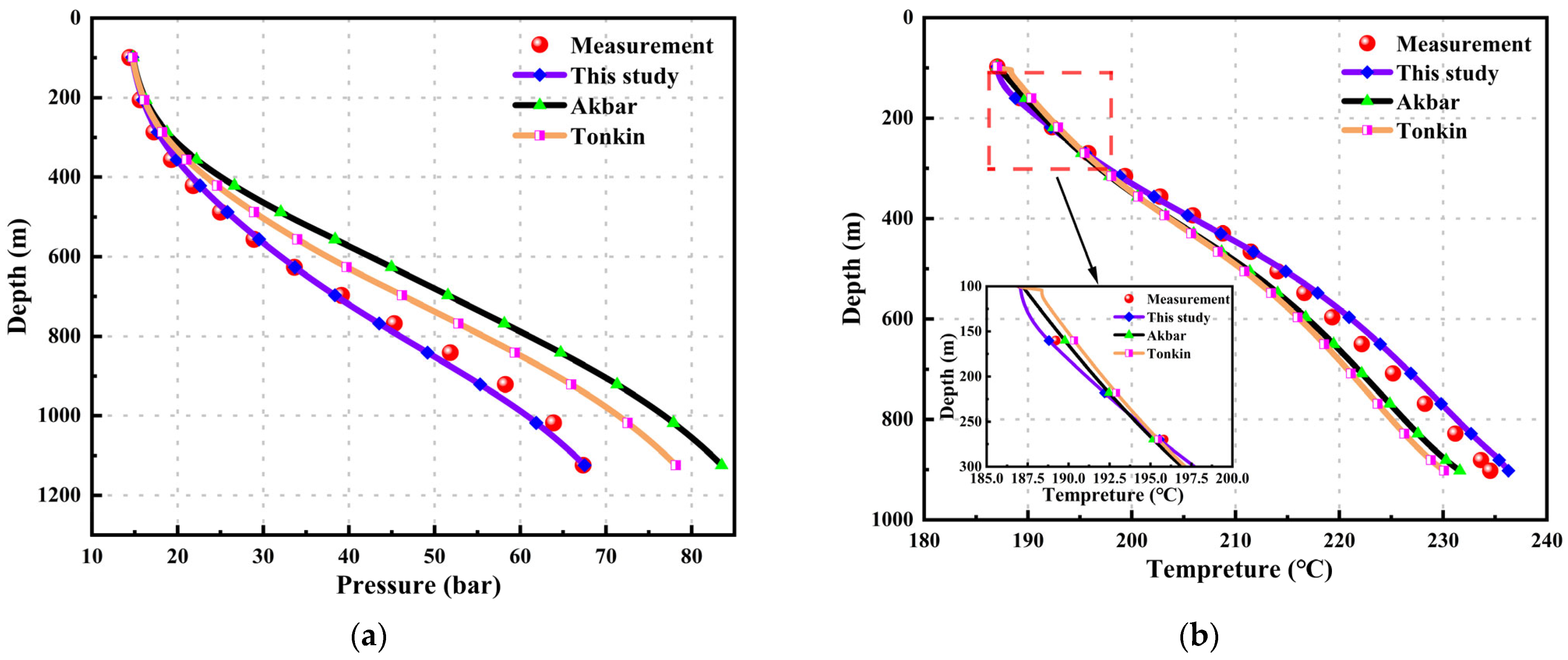
Based on the parameters of Well No. 6 as listed in Table 3, a comparison of the results calculated by the three models with the measured data is shown below:
Figure 7a shows that the pressure–depth curve of this well has two inflection points, where the rate of pressure change with depth significantly varies. The model proposed in this paper closely matches the measured data, with a calculated mean relative error (MRE) of 2.937%. The Akbar model and the Tonkin model also exhibit good pressure curves but show larger errors compared to the measured data and lag in the pressure increasing trend. The calculated MREs are 6.55% and 3.185%, respectively.
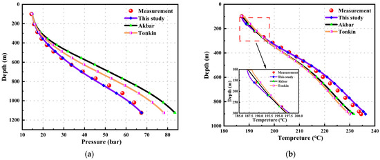
Figure 7.
Well No. 6: (a) pressure vs. depth curve; and (b) temperature vs. depth curve.
Figure 7b illustrates that the temperature calculation results of the three models have relatively small errors. However, this model has an MRE of 0.912%, which is lower than the other two models. Meanwhile, the temperature calculation results of the Akbar model are superior to those of the Tonkin model, with MREs of 1.553% and 1.814%, respectively.
5. Conclusions
This paper presents a geothermal wellbore model that demonstrates strong adaptability under three different temperature and pressure well conditions. The model integrates conservation equations with the drift-flux model and heat transfer model. After discretizing the equations, the Newton–Raphson iteration method is used to calculate the pressure and temperature. The validation results show that the model performs well in three different wellbore environments, achieving a high accuracy by taking into account multiple factors affecting the heat transfer. The experimental comparison results indicate that the model has a low mean relative error (MRE), demonstrating its high precision and reliability in calculating the bottom-hole pressure and temperature. Overall, this model provides reliable and accurate results, making it a valuable tool for optimizing the drilling parameters and ensuring drilling safety in the geothermal energy field.
Author Contributions
Conceptualization, Y.Y. and J.Z.; methodology, Y.Y.; software, Y.Y.; validation, Y.Y., X.X. and J.L.; formal analysis, L.B.; investigation, J.Z.; resources, J.L.; data curation, J.L.; writing—original draft preparation, Y.Y.; writing—review and editing, Y.Y.; visualization, J.Z.; supervision, W.L.; project administration, W.L.; funding acquisition, W.L. All authors have read and agreed to the published version of the manuscript.
Funding
This research was supported by the Special Project of Xiongan New Area of the Ministry of Science and Technology of the People’s Republic of China (2022XAGG0500).
Data Availability Statement
The data presented in this study are available upon request from the corresponding author due to privacy restrictions.
Conflicts of Interest
The authors declare no conflicts of interest.
Nomenclature
| C0 | profile coefficient |
| D | wellbore diameter, mm |
| e | specific internal energy, J/kg |
| f | wellbore friction coefficient |
| h | specific enthalpy, J/kg |
| kf | formation thermal conductivity |
| Ku | critical Kutateladze number |
| P | wellbore pressure, Pa |
| Q | energy change value, W/m2 |
| ri | wellbore radius, mm |
| Δr | difference between the wellbore radius and the drill pipe radius, mm |
| Re | Reynolds number |
| Tei | unaffected formation temperature, °C |
| Tf | fluid temperature inside the drill string, °C |
| Ta | fluid temperature in the annulus, °C |
| TD | temperature function |
| Ut | heat transfer coefficient |
| v | velocity, m/s |
| vm | mixture velocity, m/s |
| vd | drift velocity, m/s |
| vc | characteristic velocity, m/s |
| vsgf | critical velocity value, m/s |
| ρ | phase density, kg/m3 |
| α | volume fraction |
| ρm | mixture density, kg/m3 |
| ξ | wellbore roughness |
| μm | viscosity of the gas–liquid mixture, mm2/s |
References
- Bjornsson, G.; Bodvarsson, G.S. A Multi-Feedzone Wellbore Simulator. Geotherm. Resour. Counc. Trans. 1987, 11, 503–507. [Google Scholar]
- Tian, S.; Finger, J.T. Advanced Geothermal Wellbore Hydraulics Model. J. Energy Resour. Technol. 2000, 122, 142–146. [Google Scholar] [CrossRef]
- Khasani, D.K.; Itoi, R. Numerical study of the effects of CO2 gas in geothermal water on the fluid-flow characteristics in production wells. Eng. Appl. Comput. Fluid Mech. 2021, 15, 111–129. [Google Scholar] [CrossRef]
- Gao, X.; Wang, Z.-Y.; Qiao, Y.-W.; Li, T.-L.; Zhang, Y. Effects of seepage flow patterns with different wellbore layout on the heat transfer and power generation performance of enhanced geothermal system. Renew. Energy 2024, 223, 120065. [Google Scholar] [CrossRef]
- Saeid, S.; Al-Khoury, R.; Barends, F. An efficient computational model for deep low-enthalpy geothermal systems. Comput. Geosci. 2013, 51, 400–409. [Google Scholar] [CrossRef]
- Saeid, S.; Al-Khoury, R.; Nick, H.M.; Hicks, M.A. A prototype design model for deep low-enthalpy hydrothermal systems. Renew. Energy 2015, 77, 408–422. [Google Scholar] [CrossRef]
- Brown, C.S.; Falcone, G. Investigating heat transmission in a wellbore for Low-Temperature, Open-Loop geothermal systems. Therm. Sci. Eng. Prog. 2024, 48, 102352. [Google Scholar] [CrossRef]
- Zuber, N.; Findlay, J. Average volumetric concentration in two-phase flow systems. J. Heat Transf. 1965, 87, 453–468. [Google Scholar] [CrossRef]
- Hasan, A.R.; Kabir, C.S. Modeling two-phase fluid and heat flows in geothermal wells. J. Pet. Sci. Eng. 2010, 71, 77–86. [Google Scholar] [CrossRef]
- Pan, L.; Oldenburg, C.M. T2Well—An integrated wellbore–reservoir simulator. Comput. Geosci. 2014, 65, 46–55. [Google Scholar] [CrossRef]
- Akbar, S.; Fathianpour, N.; Al-Khoury, R. A finite element model for high enthalpy two-phase flow in geothermal wellbores. Renew. Energy 2016, 94, 223–236. [Google Scholar] [CrossRef]
- Tonkin, R.A.; O’Sullivan, M.J.; O’Sullivan, J.P. A review of mathematical models for geothermal wellbore simulation. Geothermics 2021, 97, 102255. [Google Scholar] [CrossRef]
- Tonkin, R.A.; O’Sullivan, J.; Gravatt, M.; O’Sullivan, M. A transient geothermal wellbore simulator. Geothermics 2023, 110, 102653. [Google Scholar] [CrossRef]
- Shi, H.; Holmes, J.A.; Durlofsky, L.J.; Aziz, K.; Diaz, L.R.; Alkaya, B.; Oddie, G. Drift-flux modeling of two-phase flow in wellbores. SPE J. 2005, 10, 24–33. [Google Scholar] [CrossRef]
- Lei, H.-W.; Xie, Y.-C.; Li, J.; Hou, X.-W. Modeling of two-phase flow of high temperature geothermal production wells in the Yangbajing geothermal field, Tibet. Front. Earth Sci. 2023, 11, 1019328. [Google Scholar] [CrossRef]
- Xu, Z.-M.; Song, X.-Z.; Li, G.-S.; Wu, K.; Pang, Z.-Y.; Zhu, Z.-P. Development of a transient non-isothermal two-phase flow model for gas kick simulation in HTHP deep well drilling. Appl. Therm. Eng. 2018, 141, 1055–1069. [Google Scholar] [CrossRef]
- Hajidavalloo, E.; Daneh-Dezfuli, A.; Falavand Jozaei, A. Effect of temperature variation on the accurate prediction of bottom-hole pressure in well drilling. Energy Sources Part A Recovery Util. Environ. Eff. 2020, 1–21. [Google Scholar] [CrossRef]
- Hasan, A.R.; Kabir, C.S. Wellbore heat-transfer modeling and applications. J. Pet. Technol. 2012, 86–87, 127–136. [Google Scholar] [CrossRef]
- Orkiszewski, J. Predicting Two-Phase Pressure Drops in Vertical Pipe. J. Pet. Technol. 1967, 19, 829–838. [Google Scholar] [CrossRef]
- Rouhani, S.Z.; Axelsson, E. Calculation of void volume fraction in the subcooled and quality boiling regions. Int. J. Heat Mass Transf. 1970, 13, 383–393. [Google Scholar] [CrossRef]
- Pan, L.; Oldenburg, C.M.; Wu, Y.-S.; Pruess, K. T2Well/ECO2N Version 1.0: Multiphase and Non-Isothermal Model for Coupled Wellbore-Reservoir Flow of Carbon Dioxide and Variable Salinity Water; Report LBNL-4291E; Earth Sciences Division, Lawrence Berkeley Laboratory, University of California: Berkeley, CA, USA, 2011. [Google Scholar]
- Hibiki, T.; Tsukamoto, N. Drift-flux model for upward dispersed two-phase flows in vertical medium-to-large round tubes. Prog. Nucl. Energy 2023, 158, 104611. [Google Scholar] [CrossRef]
- Barati, H.; Hibiki, T.; Schlegel, J.P.; Tsukamoto, N. Two-group drift-flux model for dispersed gas-liquid flow in large-diameter pipes. Int. J. Heat Mass Transf. 2024, 218, 124766. [Google Scholar] [CrossRef]
- Hibiki, T.; Ishii, M. One-dimensional drift-flux model and constitutive equations for relative motion between phases in various two-phase flow regimes. Int. J. Heat Mass Transf. 2003, 46, 4935–4948. [Google Scholar] [CrossRef]
- Bhagwat, S.M.; Ghajar, A.J. A flow pattern independent drift flux model based void fraction correlation for a wide range of gas–liquid two phase flow. Int. J. Multiph. Flow 2013, 59, 186–205. [Google Scholar] [CrossRef]
- Liu, Y.-X.; Upchurch, E.R.; Ozbayoglu, E.M. Experimental and Theoretical Studies on Taylor Bubbles Rising in Stagnant Non-Newtonian Fluids in Inclined Non-Concentric Annuli. Int. J. Multiph. Flow 2022, 147, 103912. [Google Scholar] [CrossRef]
- Harmathy, T.Z. Velocity of large drops and bubbles in media of infinite or restricted extent. AIChE J. 1960, 6, 281–288. [Google Scholar] [CrossRef]
- Fjelde, K.K.; Karlsen, K.H. High-resolution hybrid primitive–conservative upwind schemes for the drift flux model. Comput. Fluids 2002, 31, 335–367. [Google Scholar] [CrossRef]
- Lee, A.L.; Gonzalez, M.H.; Eakin, B.E. The Viscosity of Natural Gases. J. Pet. Technol. 1966, 18, 997–1000. [Google Scholar] [CrossRef]
- Chen, X.; Wang, S.-W.; He, M.; Xu, M.-B. A comprehensive prediction model of drilling wellbore temperature variation mechanism under deepwater high temperature and high pressure. Ocean Eng. 2024, 296, 117063. [Google Scholar] [CrossRef]
- Meng, L.-D.; Zhang, X.-L.; Jin, Y.-J.; Yan, K.; Li, S. Numerical simulation of fracture temperature field distribution during oil and gas reservoir hydraulic fracturing based on unsteady wellbore temperature field model. Geophysics 2024, 89, M1–M15. [Google Scholar] [CrossRef]
- Lou, W.-Q.; Sun, D.-L.; Sun, X.-H.; Li, F.-P.; Liu, Y.-X.; Guan, L.-C.; Sun, B.-J.; Wang, Z.-Y. High-precision nonisothermal transient wellbore drift flow model suitable for the full flow pattern domain and full dip range. Pet. Sci. 2023, 20, 424–446. [Google Scholar] [CrossRef]
- Liu, Y.-X.; Upchurch, E.R.; Ozbayoglu, E.M.; Baldino, S.; Wang, J.-Z.; Zheng, D.-Z. Design and Calculation of Process Parameters in Bullheading andPressurized Mud Cap Drilling. In Proceedings of the IADC/SPE International Drilling Conference and Exhibition, Stavanger, Norway, 7–9 March 2023. [Google Scholar]
- Liu, W.-Z.; Zeng, Q.-D.; Yao, J. Poroelastoplastic Modeling of Complex Hydraulic-Fracture Development in Deep Shale Formations. SPE J. 2021, 26, 2626–2650. [Google Scholar] [CrossRef]
- He, Y.-T.; Yang, Z.-Z.; Jiang, Y.-F.; Li, X.-G.; Zhang, Y.-Q.; Song, R. A full three-dimensional fracture propagation model for supercritical carbon dioxide fracturing. Energy Sci. Eng. 2020, 8, 2894–2906. [Google Scholar] [CrossRef]
- Yue, P.; Yang, H.-G.; He, C.-J.; Yu, G.-M.; Sheng, J.-J.; Guo, Z.-L.; Guo, C.-Q.; Chen, X.-F. Theoretical Approach for the Calculation of the Pressure Drop in a Multibranch Horizontal Well with Variable Mass Transfer. ACS Omega 2020, 45, 29209–29221. [Google Scholar] [CrossRef]
- Garg, S.K.; Pritchett, J.W.; Alexander, J.H. Development of New Geothermal Wellbore Holdup Correlations Using Flowing Well; Idaho National Lab. (INL): Idaho Falls, ID, USA, 2004. [Google Scholar] [CrossRef]
- Zolfagharroshan, M.; Khamehchi, E. A rigorous approach to scale formation and deposition modelling in geothermal wellbores. Geothermics 2020, 87, 101841. [Google Scholar] [CrossRef]

Disclaimer/Publisher’s Note: The statements, opinions and data contained in all publications are solely those of the individual author(s) and contributor(s) and not of MDPI and/or the editor(s). MDPI and/or the editor(s) disclaim responsibility for any injury to people or property resulting from any ideas, methods, instructions or products referred to in the content. |
© 2024 by the authors. Licensee MDPI, Basel, Switzerland. This article is an open access article distributed under the terms and conditions of the Creative Commons Attribution (CC BY) license (https://creativecommons.org/licenses/by/4.0/).