Abstract
The operation envelope of distribution networks can obtain the independent p-q controllable range of each active node, providing an effective means to address the issues of different ownership and control objectives between distribution networks and distributed energy resources (DERs). Existing research mainly focuses on deterministic operation envelopes, neglecting the operational status of the system. To ensure the maximization of the envelope operation domain and the feasibility of decomposition, this paper proposes a modified hyperellipsoidal dynamic operation envelopes (MHDOEs) method for distribution networks based on adjustable “Degree of Squareness” hyperellipsoids. Firstly, an improved convex inner approximation method is applied to the non-convex and nonlinear model of traditional distribution networks to obtain a convex solution space strictly contained within the original feasible region of the system, ensuring the feasibility of flexible operation domain decomposition. Secondly, the embedding of the adjustable “Degree of Squareness” maximum hyperellipsoid is used to obtain the total p-q operation domain of the distribution network, facilitating the overall planning of the distribution network. Furthermore, the calculation of the maximum inscribed hyperrectangle of the hyperellipsoid is performed to achieve p-q decoupled operation among the active nodes of the distribution network. Subsequently, a correction coefficient is introduced to penalize “unknown states” during the operation domain calculation process, effectively enhancing the adaptability of the proposed method to complex stochastic scenarios. Finally, Monte Carlo methods are employed to construct various stochastic scenarios for the IEEE 33-node and IEEE 69-node systems, verifying the accuracy and decomposition feasibility of the obtained p-q operation domains.
1. Introduction
In response to the national dual carbon goals, in recent years, there has been a high penetration of distributed energy resources (DERs) in distribution networks, accompanied by a significant increase in flexible and controllable resources [1,2]. Consequently, the operational risks of the systems have risen sharply. However, there are differences in the focus of control between the dispatch center and DERs. The dispatch center primarily coordinates system operations while satisfying constraints for safe operation, while DERs primarily aim to maximize their own benefits. There is some conflict between the two parties during operation. To achieve safe and reliable operation of the distribution network and flexible control of controllable resources, it is particularly important to carry out precise calculations of the operating domains [3] of each active node (i.e., nodes connected to flexible and controllable resources such as DERs) in the distribution network, and to achieve decoupled operation of each active node by controlling the output of flexible resources, such as distributed generation at each node.
In order to achieve the safe and reliable operation of the distribution network and the flexible regulation of controllable resources, the operation domain [3] of each active node in the distribution network (that is, nodes that flexibly regulate resources such as access to DERs) is accurately calculated, and the decoupling operation of each active node is realized by controlling the output of each node’s flexible resources, such as distributed power supply.
The relevant literature proposes reactive voltage [4], active voltage [5], sag control curves, and reactive–active cooperative control strategies [6] for the direct control of DERs, enabling them to satisfy the safe operation constraints of the distribution network. However, it is challenging to monitor the operation status of DERs in real time [7].
The authors of [8] proved for the first time the existence of all distribution network security operation domains and provided a strict definition thereof. The calculation of the safe operating domain for distribution networks relies on the precise localization of stable operating boundaries. The authors of [9] gradually observed the system’s operating status to obtain the local boundaries of the safe operating domain in distribution networks, while [10] obtained a collection of flexible operating points for DERs in terms of active and reactive power through extensive simulations of practical application scenarios using the Monte Carlo method. In [11], the problem of determining the critical point of stable operation of the system is transformed into the problem of finding the optimal solution, and the piecewise linearization method is used to fit the security domain boundary and generate the observable security domain space.
However, the above study cannot fit the boundary of the operation domain more accurately, and the related study [12] further proposes using the dynamic operation envelopes (DOEs) method of the distribution network operation domain to compute the safe operation domain of the distribution network. The solution of the flexible operation domain of distribution networks needs to follow two principles: one is to maximize the volume of the operating domain under the premise of approaching the actual solution, in order to improve the utilization rate of system capacity and ensure the flexible operation of the system; the other is to ensure the decomposition feasibility of the resulting operation domain, i.e., without violating the operation constraints of the network or the DERs, a complete trajectory of the total power in the feasible region can be obtained by appropriately scheduling the DERs.
The papers [13,14] are based on the exact unbalanced three-phase power flow method. On the premise of ensuring safe system operation, this method gradually adjusts the input or output power of fixed loads according to the system’s operating status [15]. However, the method involves multiple iterations, the safe operating domain enveloped is conservative, and the conservative use of the network capacity leads to the waste of system resources [16,17,18]. Some scholars have proposed a method based on the unbalanced three-phase optimal power flow (UTOPF) computation [19], which takes the maximum of the scheduling region as the objective function to obtain the allowable regulation range of DERs. However, this method sacrifices the accuracy of running domain calculations. To solve the problem that UTPF and UTOPF methods are too conservative or have low solution accuracy, [20] collected a large amount of system data and used machine learning algorithms to fit a black-box model of the system for predicting DERs. However, this type of method relies on the accuracy and real-time nature of the data.
Existing studies mainly use conventional parameterized convex sets to fit the flexible operation domain of distribution networks; however, due to the randomness of DERs and the diversity of distribution network equipment, this method has poor adaptability to complex and stochastic scenarios, leading to the intensification of the system security risk during network operation. Considering that the ellipse has high adaptability and can dynamically adjust its parameters to change its size and shape, adapting to different operating states of the system, [21] proposes the p-q optimal elliptic safe operation domain envelope method for distribution networks with time decoupling, but this method only provides the total safe operation domain for the system operation, and it cannot provide the safe operation range for each active node separately. The authors of [22] constructed a rotating rectangular model for the operating envelope for each active node to obtain the p-q flexible operating domain between each active node, but the p-q of each active node cannot be independently regulated and cannot provide a specific scheduling scheme for the distribution network.
The operating domains of the active nodes in the distribution network exist in different spaces, and mapping from high-dimensional feasible domains to low-dimensional ones can result in the loss of depth information. However, most current research focuses on low-dimensional operating domains, which can easily lead to system violations [23,24,25] even when all active nodes follow the calculated flexible operating domains.
To solve the above problems, this paper first adopts the improved convex inner approximation method to obtain the convex solution space strictly contained in the original feasible region of the system, so as to ensure the feasibility of the flexible operation domain decomposition of the distribution network under the high proportion of new energy penetration. In order to avoid the loss of depth information accompanied by the mapping of the high-dimensional feasible domain to the low-dimensional one, a superellipsoid is proposed to obtain the maximum inner connected super-rectangle of the multidimensional feasible domain, and to realize p-q decoupling of the operation between each active node of the distribution network. A “Degree of Squareness” adjustable superellipsoid with higher adaptability is further proposed to envelope the flexible operation domain of the distribution network, which is closer to the optimal solution while achieving a pre-specified level. In view of the randomness of DERs and the diversity of distribution network equipment, a penalty term is added to the objective function considering the running state of each node to improve the applicability of the model to calculate multiple scenarios. Finally, for IEEE 33-node and IEEE-69 node systems, the Monte Carlo method is used to construct a variety of random scenarios, and the accuracy and decomposition feasibility of the p-q running domain are verified.
The remainder of this paper is structured as follows: Section 2 examines the use of an improved convex inner approximation method to obtain a convex solution space within the original feasible region of the distribution network, ensuring the feasibility of decomposing the flexible operation domain of the distribution network. Section 3 proposes a new flexible envelope method for the operation domain of distribution networks based on adjustable “Degree of Squareness” hyperellipsoids. Section 4 presents the simulations and analysis, while Section 5 provides the conclusions.
2. Feasible Domain Modeling Based on Network Operational Constraints
The active distribution network model encompasses multiple sets of constraints, with the power flow constraints exhibiting non-convex nonlinearity [26]. To ensure the feasibility of decomposing the flexible operation domain of the distribution network, it is crucial to rewrite the original distribution network model.
2.1. Rewriting of the Power Flow Model of the Distribution Network
Although the traditional distribution network model convex relaxation method [27,28,29] provides a good solution space for distribution network optimization, it cannot guarantee that the model is strictly contained in the original feasible region of the system, and the boundary conditions are often difficult to meet. Therefore, this paper introduces an improved convex inner approximation method to obtain a convex solution space strictly contained in the original feasible region of the system.
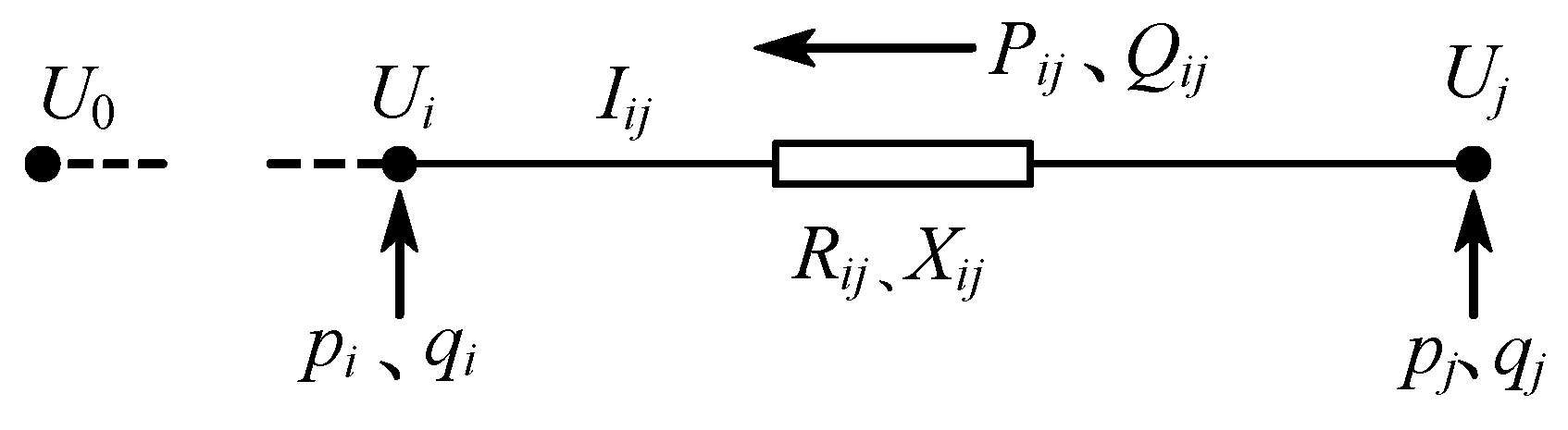
A feeder line of a distribution network is generally expressed, as shown in Figure 1.
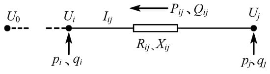
Figure 1.
Radial network equivalent model.
In Figure 1, U0 is the voltage of the first node; Ui and Uj are the voltage of node i and j, respectively; and are the net injected active and reactive power, respectively, at node i; and are the active and reactive power of branch ij, respectively; is the current of branch ij; and Zij = Rij + jXij is the impedance of branch ij.
In this paper, , , , and reference [30] were used to process the original distribution network model, and the following results were obtained:
where ; ; ; ; ; ; is the association matrix of nodes and branches; and the matrix (I − A) is invertible [30].
The variables P and Q are coupled to each other [31,32], and the rest of the variables except for the branch currents are decision or state variables, using I as an intermediate quantity to denote the other variables.
Using p and l as decision quantities, the upper and lower bounds for each proxy variable can be obtained:
where DX+ is a non-negative element in matrix DX; ; DX− is a negative element in DX; ; and are the maximum and minimum values of l(p), respectively; and , .
The state variables P and Q are functions of the branch currents l. Therefore, the accuracy of the relaxation depends on the values of the upper and lower bounds of l. The relaxation bounds of l will be illustrated below.
For the branch ij, the second-order Taylor expansion of the branch power flow rate based on the rated operating point of the system is given by the following expression:
where indicates when the system is at the rated operating point, while the matrices , , and are defined in reference [33]:
The derivation of the upper and lower bound expressions for l is shown below:
where J+ and J− are matrices consisting of non-negative and negative elements in J, respectively, while δ+ and δ− are matrices consisting of non-negative and negative elements in δ, respectively. lmin may be negative, but , so the lower bound of lij should take the value of max{0,lmin}.
After defining the upper and lower bounds of l, P and Q can be replaced by proxy variables to obtain a convex solution space inside the initial non-convex region.
2.2. Distribution Network Constraints
The following constraints need to be met for distribution network operation:
where: is the upper limit of the branch current amplitude; and are the voltage amplitudes at nodes i and j, respectively; and are the upper and lower limits of the node voltage amplitudes, respectively; and are the active and reactive powers of the branch ij, respectively; and are the upper and lower bounds of the active power of the branch ij, respectively; Gij is the conductance of the line ij; θij is the phase-angle difference between the voltages at nodes i and j; is the apparent power; is the active power injected by the power supply at node i, and is the active power consumed by the load at node i; is the reactive power injected by the power supply at node i, and is the reactive power consumed by the load at node i.
3. Construction and Improvement of Flexible Operational Domain Models
Due to the loss of depth information accompanying the mapping from high-dimensional feasible regions to lower dimensions, even if all active nodes are located within the calculated flexible operation domain, the network may still face operational safety risks. Therefore, when using polygon or ellipse approximation methods to solve for the flexible operation domain of the distribution network, the obtained capacity allocation schemes may not all be practically feasible.
3.1. Distribution Network Operating Envelope Definition
The feasibility region (FR) model developed above, denoted as , is represented as follows:
where: p = {P1, …, Pn}, and q = {q1, …, qn}; p and q are the variables corresponding to the active and reactive power to be optimized, respectively; is the vector consisting of all the variables of the distribution network (including state and control variables); , , , , , and are the constant parameter matrices of suitable size, and ; indicates all distribution network operation constraints, including the voltage amplitude and current amplitude constraints of distribution lines.
provides a guideline for the safe operation [34,35] of the distribution network; however, the high penetration rate of resources such as DERs exacerbates the risks associated with active distribution network operations. Issues like voltage overruns and line overloads become prominent, and to achieve practicality within this feasible domain, it is necessary to consider the coupling between controllable resources at each node of the distribution network [36,37].
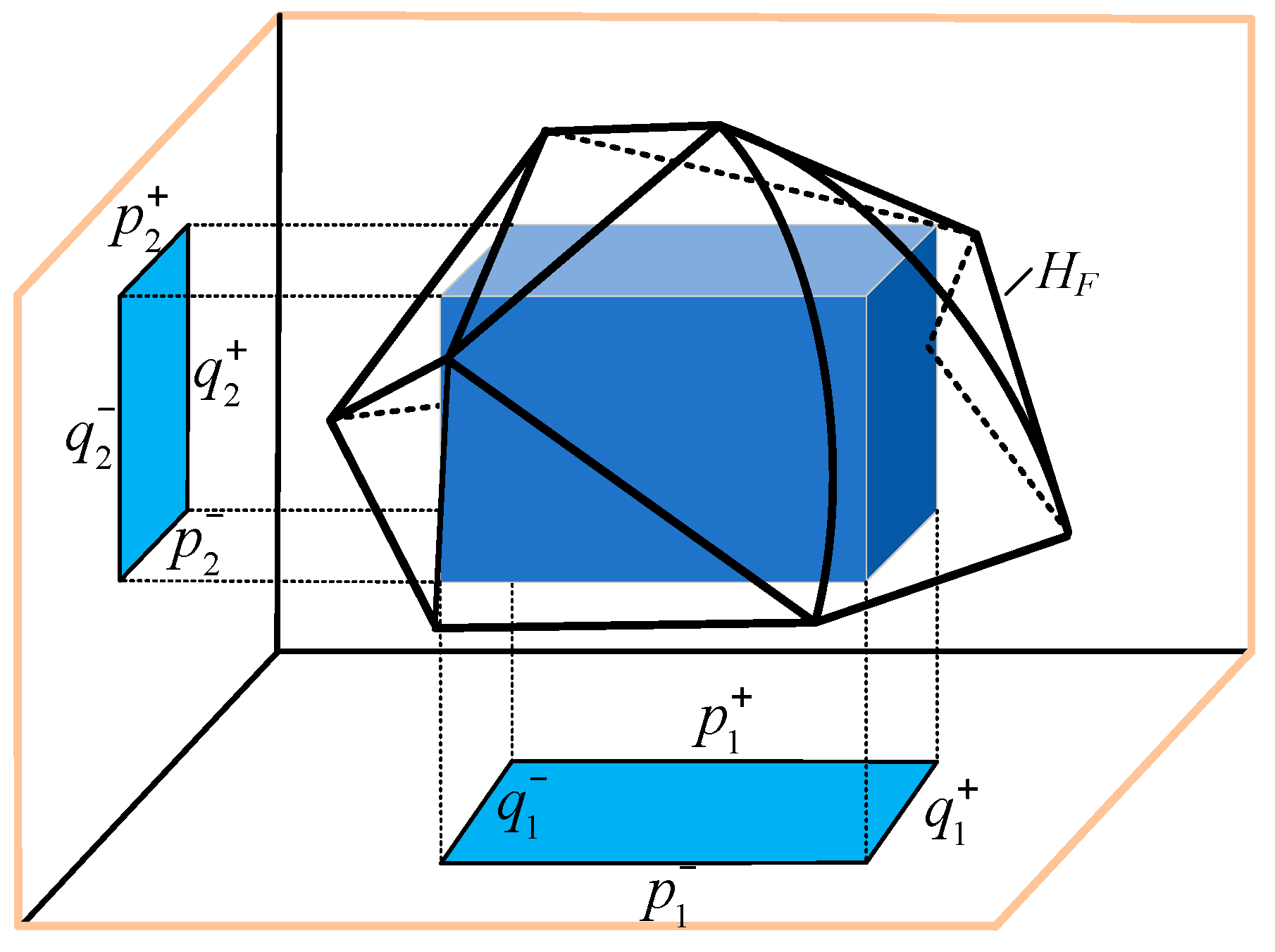
In this paper, we aim to find a decoupled feasibility region (DFR) within the convex solution space of the original feasible region of the system, which allows p-q independent scheduling among active nodes, and each active node can control its power independently within the boundary of the DFR without violating the network operation constraints, so as to achieve the decoupled operation of each active node in the active distribution network. The DFR is represented as a hyperrectangle in multidimensional space, and Figure 2 shows the schematic diagram of the decoupled p-q operation domain between active node 1 and active node 2, where is the high-dimensional feasible domain space. From the perspective of spatial geometry, the power planes of each active node should be orthogonal to each other [22].

Figure 2.
A p-q decoupling diagram between active nodes.
The mathematical expression for the hyperrectangle is as follows:
where is the th active node of the distribution network; and are the upper and lower bounds of active power after decoupling of node , respectively; and are the upper and lower bounds of reactive power after decoupling of node , respectively.
3.2. Tunable Superellipsoid Running Envelope Solution Model Based on “Degree of Squareness”
Due to the loss of depth information associated with the mapping from high-dimensional to low-dimensional feasible domains, the network may still face the risk of safe operation even if all active nodes are located in the calculated flexible operation domain. Therefore, the capacity allocation schemes obtained by using polygon or ellipse approximation methods to solve the flexible operation domain of the distribution network may not all be practical and feasible.
As shown in Figure 3, the blue “*” indicates the baseline operating point, and the red “*” indicates the actual operating point. it is assumed that active nodes 1 and 2 have operation points and , respectively, at a certain moment, both of which are located in their respective flexible operation domains, but the risk of voltage overrun still occurs for the system. The process of mapping the high-dimensional model to the low-dimensional model is irreversible with missing depth information.
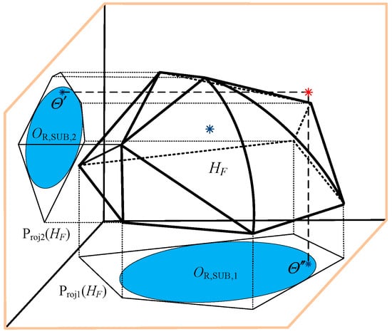
Figure 3.
Run domain assignment: non-feasible example.
In Figure 3, Proj1 and Proj2 are its mappings on different low-dimensional running domain spaces for three-dimensional examples, while OR,SUB are the ellipsoidal running domains obtained from the low-dimensional feasible domain approximation.
Aiming at the above problems, this paper proposes a flexible operation domain envelopment method based on hyperellipsoids to avoid the loss of depth information due to dimensionality reduction; by embedding the maximum hyperellipsoid in the polyhedron FR in order to obtain the maximum hyperrectangle, we achieve the p-q decoupled operation among the active nodes of the power distribution network.
The hyperellipsoid is essentially a stretching transformation of the unit sphere, with the following formula:
where ω is the coordinate vector of the point inside the superellipsoid, is the center of the superellipsoid, and L is a positive definite − 1-dimensional diagonal matrix representing the lengths of all axes of the ellipsoid.
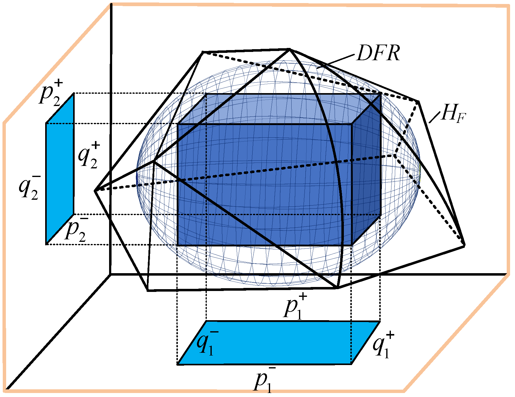
Figure 4 shows the schematic diagram of the flexible operation domain envelope method based on the superellipsoid, which first searches for a maximal superellipsoid within the convex solution space of the original feasible region of the system to obtain the total p-q operation domain of the distribution network, which is convenient for the overall planning and operation of the distribution network, and further calculates the maximal internally connected super-rectangles of the superellipsoid, which achieves the decoupling of the p-q operation among the active nodes.
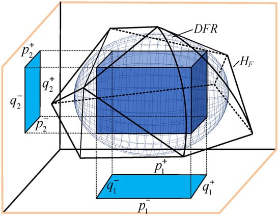
Figure 4.
Dynamic operation envelope method based on hyperellipsoids.
Assuming that the coupling of multiple active nodes is not considered in this paper, the ellipsoid approximation method has a good envelope for the two-dimensional flexible operation domain projected by an active node, but the actual operation of the system needs to take into account the coupling of multiple active nodes in order to determine the feasibility of the capacity allocation scheme; therefore, the construction of a high-dimensional p-q operation domain is particularly important. According to the existing studies, the three-dimensional running domain derived from multiple sets of two-dimensional p-q elliptic running domains is not necessarily a standard ellipsoid but, rather, an ellipsoid with “square degree”. This conclusion can be extended to higher dimensions.
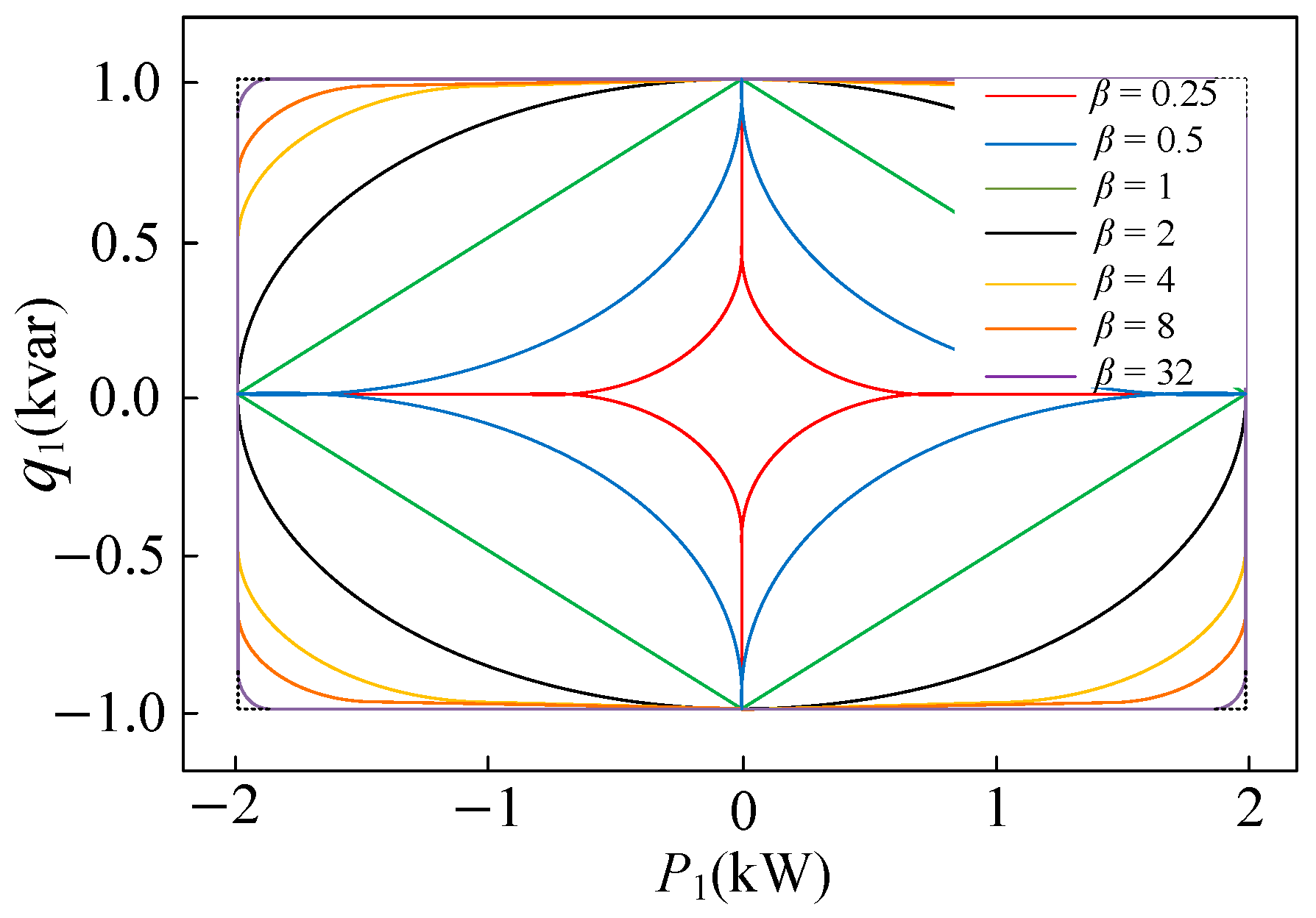
From the above analysis, the dynamic envelope of the flexible operation domain of the distribution network considering the “Degree of Squareness” adjustable superellipsoid can be closer to the optimal solution based on reaching the pre-specified level. Figure 5 shows the power boundary curves of the active nodes with different squareness parameters . The power curves are convex when and are closer to the rectangle as increases.
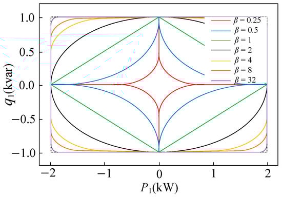
Figure 5.
The concept of a “square” adjustable hyperellipsoid.
Consider the “Degree of Squareness” adjustable hyperellipsoid, which can be expressed as follows:
In this paper, the squareness parameter is adjusted in order to expand the volume of the superellipsoid, but the volume of the superellipsoid changes slowly as the parameter becomes larger, so in this paper we take (K is a positive integer), and the superellipsoid equation is further expressed as follows:
where is the set of constraints, where is an intermediate vector variable, is the ith element of , and contains mK + 1 quadratic constraints.
Using the “Degree of Squareness” adjustable hyperellipsoid parameters, the formula for the volume of the tangent hyperrectangle is obtained as follows:
where is the ith element of .
The optimal solution is denoted when the volume of the interior hyperrectangle is maximized:
where is the surface of the “square” adjustable hyperellipsoid.
The hyperellipsoid’s internal tangent hyperrectangle can be re-expressed as follows:
Most of the existing studies ignore the operation state of each active node, and the solved operation domain is fixed. In order to reflect the flexibility of the operation domain solution and weaken the unfavorable effects of the uncertainty and complexity of resources such as DERs, this paper presents the following discussion:
(1) Disregarding node operational states
The problem of computing the maximum internally connected hyperrectangle of a hyperellipsoid can be expressed as follows:
where and are the upper and lower bounds of the active power constraints, respectively, while and are the upper and lower bounds of the reactive power constraints, respectively.
(2) Consideration of node operational state
When the operating state of the node is unknown, introduce correction coefficients , penalizing in the objective function to ensure that the inputs and outputs are as equal in magnitude as possible and Vh can be maximized as follows:
where is the correction coefficient, is the slack variable introduced by considering the operating state of the node, is the ith element of the vector , is a 0–1 variable denoting the operating state of node i, = 1 denotes the input power, = −1 denotes the output power, and is the proposed input/output limit to be assigned to each node.
Formula (19) Constraint (3) ensures that the limit of output power is as close to 0 kW as possible when the node inputs power, and the limit of input power is as close to 0 kW as possible when the node outputs power, so that the node can freely vary its power between 0 kW and the assigned capacity limit. For example, if the node is outputting power, it will be penalized as its input limit in the objective function. Then, consider the operational state of the customer after replacing n with 2K.
The upper and lower limits of the capacity of the active node are denoted as follows:
where and need to be optimized.
For the uncertain in (19), a generalized formula for the maximum value of is derived in order to enable it to express the general case of distribution network operation:
where is a known vector, a row of ; and are Lagrange multipliers.
The Lagrange function of Equation (22) is
Then, is an equivalent problem of Formula (22), which can be further expressed as follows:
By introducing the intermediate variable , replacing x with , and removing the minimum operator in the objective function of Formula (24), Formulas (18) and (19) can be reformulated as follows:
where [·]m denotes the mth row of the matrix or the mth element of the vector, and [·]m,i denotes the (m, i)th element of the matrix.
The corresponding maximum internally connected super-rectangle is obtained by solving the above formulas:
where and are the maximal hyperrectangles and , respectively, and , corresponding to the maximal hyperellipsoid at its maximum.
4. Experimental Verification
In this paper, IEEE 33-node and IEEE 69-node systems were used for simulation and analysis, the system topology and related parameter settings were derived from the literature [38,39], and the Monte Carlo method was used to construct a variety of stochastic scenarios to verify the accuracy of the resulting p-q operation domain of each active node and the feasibility of decomposition. The IEEE 33-node system used in this paper selects nodes 6, 13, 9, 24, 30, and 33 as active nodes, while the IEEE 69-node system selects nodes 4, 8, 21, 25, 36, 40, 45, 48, 52, and 60 as active nodes. The specific configurations of the IEEE 33-bus system and the IEEE 69-bus system are detailed in Appendix A.
Line loss is not considered in this study, so the line power flow constraint depends on the network structure. The reference capacity of all examples was set to 10 MVA, and the node voltage constraint ranged from 0.95 p.u. to 1.05 p.u. The CONOPT solver in GAMS 31.1.1 software was used to obtain the security domain boundary points. The hardware environment of the test system was an AMD A10-8700P 1.80 GHz processor by AMD (Santa Clara, CA, USA), and the memory capacity was 8 GB.
4.1. Total Operational Domain Envelope Security Assessment
Taking the IEEE 33-node system as an example, 1000 actual operating points were randomly selected during the whole time period of the distribution network to analyze the coverage of the actual operating points by the superellipsoid enveloping method and the adjustable superellipsoid enveloping method with the “Degree of Squareness” compared with the traditional convex dynamic operation envelopes (CDOEs) [40]. Considering that there are errors in the prediction of the actual operation scenarios of the system, this paper improves the prediction accuracy requirement by setting the maximum of hazardous scenarios to not exceed 5%.
Figure 6 shows the actual operating point coverage of the IEEE 33-node system based on the CDOEs approach. Most of the actual operating points in the analyzed high percentage penetration of distributable power are located inside and on the boundaries of the operating domain of the envelope, where 14% of the actual operating points are located outside the operating domain, exceeding the upper limit of the hazardous scenario setup.
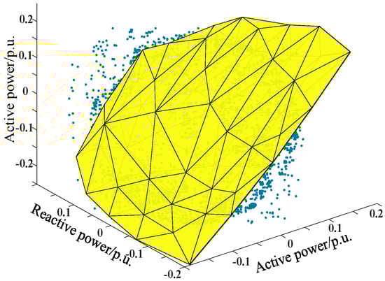
Figure 6.
Envelope of actual running points for the CDOEs method.
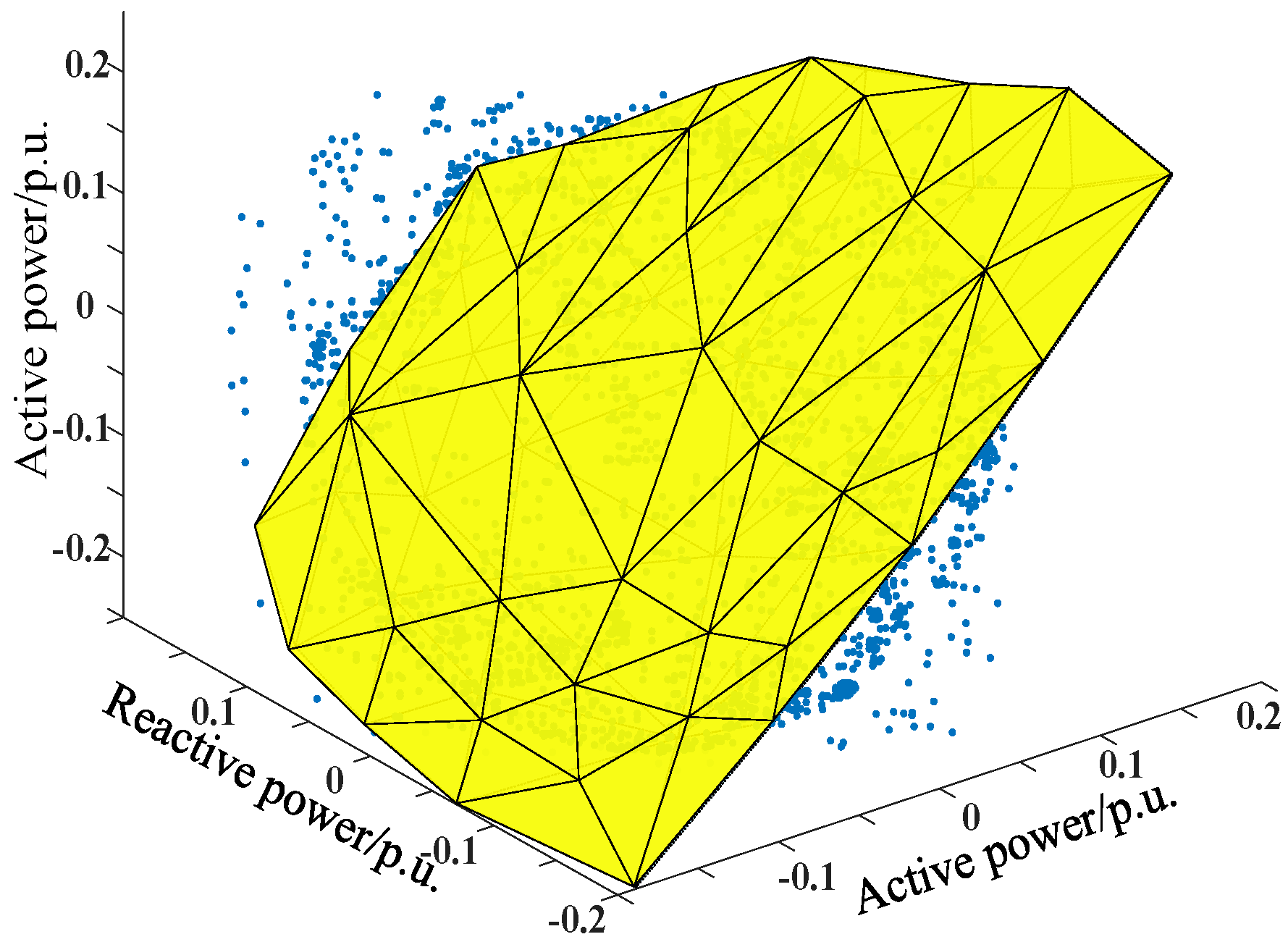
Figure 7 shows the running domain covering the actual running points enveloped by the HDOEs method adopted in this paper, and the analysis shows that the running domain established by the HDOEs method can cover 91% of the actual running points, which is an overall improvement of about 5% compared with the effect of the CDOEs method.
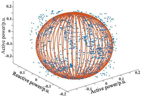
Figure 7.
Envelope of actual running points for the HDOEs method.
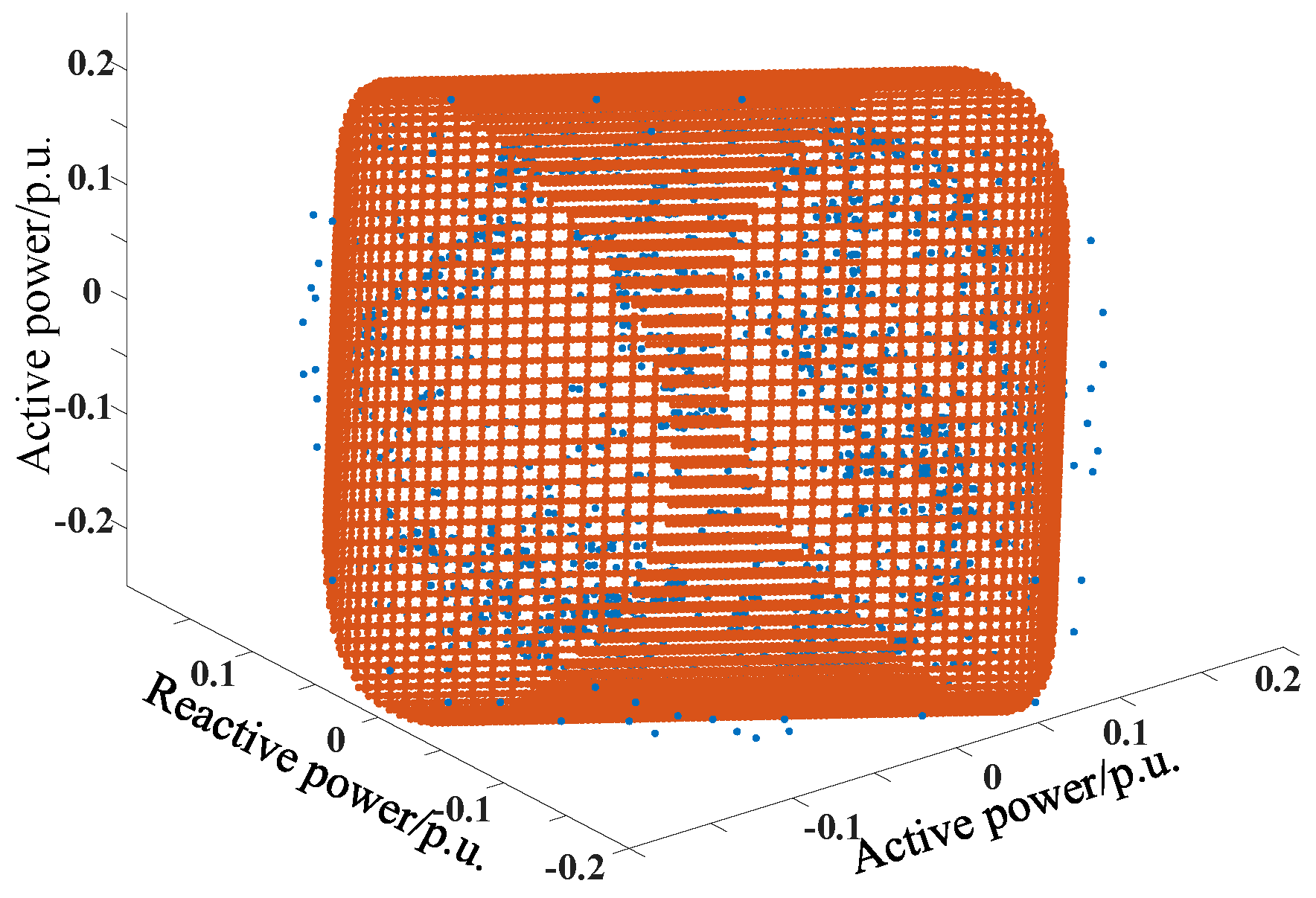
In order to obtain higher envelope accuracy and a larger envelope range, we added the “Degree of Squareness” on the basis of the HDOEs method, and Figure 8 shows the HDOEs method with an adjustable “Degree of Squareness” on the envelope of actual operating points, which is able to cover 97% of the selected actual operating points, while the envelope range is further improved by about 6% to meet the maximum upper limit of hazardous scenarios set by the system.
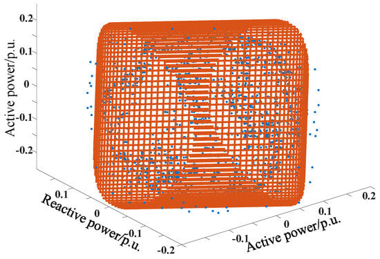
Figure 8.
The envelope of actual operating points for the MHDOEs method.
4.2. Active Node Independent Regulatory Scope Analysis
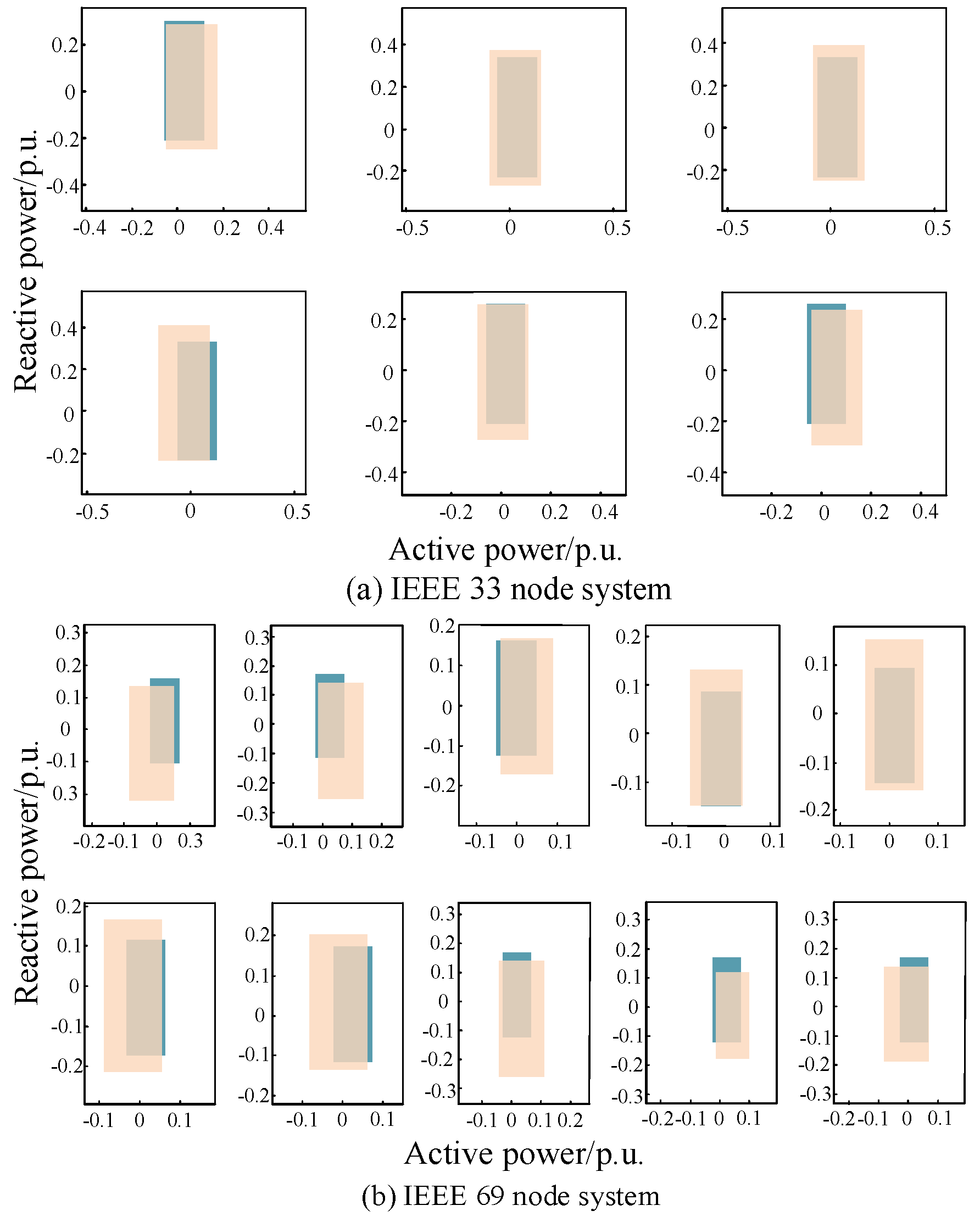
The envelope of the distribution network operation domain needs to maximize the operation domain in close proximity to the actual solution in order to improve the utilization of the system capacity as well as the flexibility of the operation. Figure 9 compares the p-q operation domains of each active node generated by the rectangular DOEs (RDOEs) [22] method with the method proposed in this paper.
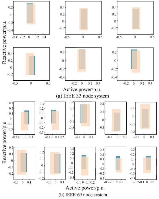
Figure 9.
Comparison of p-q operating domains of active nodes generated by different methods.
The blue color in Figure 9 shows the area covered by the rectangular envelopment method, while the light orange color shows the area covered by the method proposed in this paper. Figure 9a shows the p-q operation domain range of 6 active nodes of the IEEE 33-node system, while Figure 9b shows the p-q operation domain range of 10 active nodes of the IEEE 69-node system, and both methods ensure that the benchmark operation point is within the feasible domain of the enveloped area.
Figure 10 shows the area analysis of the operating domains enveloped by different methods. Compared with the conventional RDOEs method, the HDOEs method proposed in this paper increases the operation envelope area, with an average enhancement effect of 144.82% for the IEEE 33-node system and 131.21% for the IEEE 69-node system. By using MHDOEs to correct the operation domains encompassed by the HDOEs method, the IEEE 33- and 69-node systems’ envelope areas are further improved by 9.87% and 1.37%, respectively.
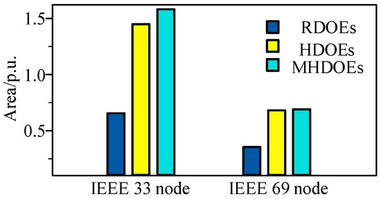
Figure 10.
Different methods to run the envelope area comparison.
The above analysis verifies that the p-q operation domain envelopment method based on the “Degree of Squareness” adjustable superellipsoid can expand the operation domain on the basis of the existing method, providing more operable p-q adjustment ranges for the active nodes, and the operation domain areas of the active nodes enveloped by the method in this paper do not differ much, which is in line with the actual operation situation.
Table 1 shows the average errors generated by the RDOEs method, HDOEs method, and MHDOEs method applied to the operating domain envelope of the IEEE 33-node system and the IEEE 69-node system.

Table 1.
Comparison of envelope mean error of different methods.
As can be seen from Table 1, compared with the conventional RDOEs method, the HDOEs method proposed in this paper improves the accuracy of the operational envelope, where the average error of the IEEE 33-node system is reduced by 0.12, and that of the IEEE 69-node system is reduced by 0.1. Using MHDOEs to modify the operating domain enclosed by the HDOEs method, the envelope area of the IEEE 33- and 69-node systems is further reduced by 0.08 and 0.11, respectively, so the security domain constructed by the method in this paper is more accurate.
4.3. Operational Domain Envelope Time Analysis
Table 2 shows the analysis of the runtime domain computation time for different methods.
Table 2.
Different methods to run envelope time analysis.
By analyzing Table 2, it can be seen that the HDOEs method and MHDOEs method proposed in this paper directly envelope the operational domain in high-dimensional space; thus, compared with the conventional RDOEs method, the calculation time of the operational domain is longer, and the calculation time is slightly increased compared with the RDOEs method but still remains at a small order of magnitude. The calculation time of the operational domain meets the needs of the calculation of the operational domain of the distribution network. Moreover, for the IEEE 33- and 69-node systems, the operating domain can be maximized on the premise of ensuring model accuracy, and the distribution network resources can be flexibly regulated under the high proportion penetration of DERs.
4.4. Operational Domain Envelope Security Validation
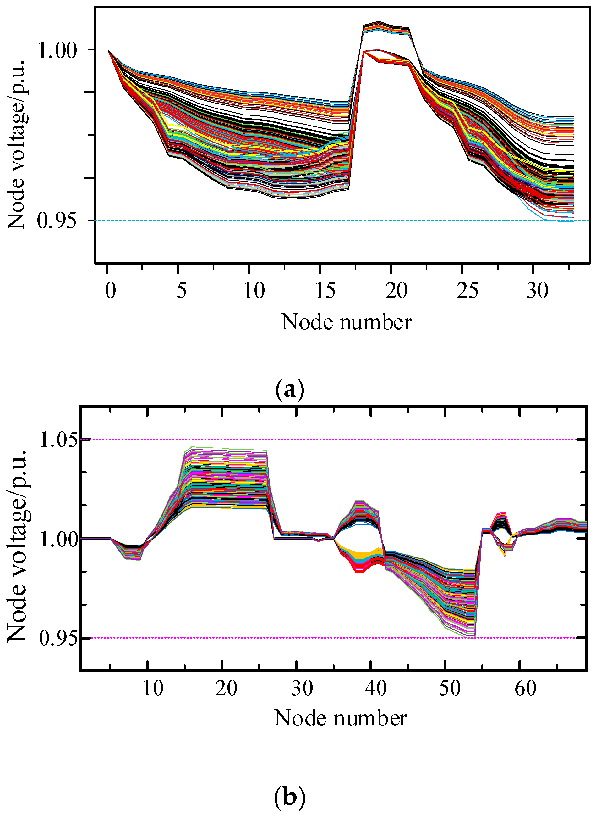
While verifying the accuracy of the envelope method in this paper, it is also necessary to verify the security of each actual operation point in the operation domain; in this paper, the Monte Carlo method is used to simulate the actual operation of the distribution network, the flexible resources (such as DERs) of each active node are controlled to satisfy the active–reactive power of randomly selected operation points, the power of the baseline operation point is used as the injected power of the nodes (except for the active node), and we analyze whether the voltage of each node overruns the limits.
Figure 11 shows the node multi-scenario voltage fluctuation curves for the IEEE 33-node and IEEE 69-node systems.
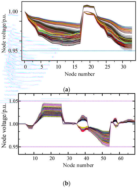
Figure 11.
Run envelope security verification: (a) IEEE 33-node system voltage fluctuation curve; (b) IEEE 69-node system voltage fluctuation curve.
The results show that there is no overrun in the voltage of each node within the flexible operation domain of the DOEs methodology envelope, as shown in Figure 11. It is able to ensure the safe operation of the distribution network.
5. Conclusions
This paper proposes a dynamic envelope method for the operation domain of distribution networks using an adjustable “degree of squareness” superellipsoid, which achieves p-q decoupling operation among various active nodes in the distribution network. This provides an effective means to address the issues of different ownership between distribution networks and distributed energy resources (DERs) and discrepancies in control objectives. Furthermore, considering the operating states of the distribution network, a margin measure with a penalty term was added to the model to enhance the network applicability of the proposed method. Finally, simulation analyses were conducted on the IEEE 33-node and IEEE 69-node systems, leading to the following conclusions:
- (1)
- The method adopted in this paper uses an improved convex inner approximation approach, providing a convex solution space that is strictly contained within the original feasible region of the system for subsequent envelope construction of the distribution network operation domain.
- (2)
- This paper employs a “degree of squareness” adjustable superellipsoid envelope method with high network adaptability, capable of dynamically adjusting parameters to change its size and adapt to different operating states of the system, achieving p-q decoupling operation among various active nodes in the distribution network. Compared with traditional methods, the proposed method significantly enhances the range of the operation envelope while ensuring the feasibility of solution decomposition.
- (3)
- In response to the high penetration of DERs, compared with traditional convex envelope methods, this paper’s method adds a penalty term to the model to penalize unknown states of each node during the calculation of the operation domain, effectively mitigating the adverse effects brought by the uncertainty and complexity of resources such as DERs.
The method proposed in this paper can adjust the shape and size of the envelope by changing the envelope parameters according to the operating state of the system, and it introduces the margin measure with a penalty term. This flexibility is an important embodiment of the extensibility of the method. In the future, the design of envelope parameters and margin metrics could be further strengthened to consider more types of system disturbances and uncertainties, such as weather changes, equipment failures, etc., to enhance the robustness and practicability of the method.
Author Contributions
Investigation, Y.H.; Project Administration, Y.H.; GAMS 31.1.1 software, K.W., J.X., and Y.L.; Supervision, Y.H.; Visualization, J.X.; Writing—Original Draft, K.W. All authors have read and agreed to the published version of the manuscript.
Funding
This work was sponsored by the National Natural Science Foundation of China (52107101), Priority Academic Program Development of Jiangsu Higher Education Institutions (PAPD2024), and Science and Technology Project of State Grid Jiangsu Electric Power Co., Ltd. (J2020014).
Data Availability Statement
The original contributions presented in the study are included in the article.
Conflicts of Interest
The authors declare no conflict of interest. The funder was not involved in the study design, collection, analysis, interpretation of data, the writing of this article or the decision to submit it for publication.
Nomenclature
The following are some of the symbols and abbreviations used in this text:
| Symbol | |
| Mathematical expression of feasible domain | |
| The set of all run constraints | |
| Mathematical expression of hyperrectangle | |
| L | The length of all axes of a hyperellipsoid |
| Hyperellipsoid with adjustable “square” | |
| Built-in hyperrectangular volume | |
| Introduced relaxation variable | |
| The input/output quota to be allocated by each node | |
| Abbreviations | |
| DERs | Distributed energy resources |
| DFR | Decoupled feasibility region |
| UTOPF | Unbalanced three-phase optimal power flow |
| DOEs | Dynamic operation envelopes |
| CDOEs | Convex DOEs |
| RDOEs | Rectangular DOEs |
| HDOEs | Hyperellipsoidal DOEs |
| MHDOEs | Modified HDOEs |
Appendix A
Figure A1 is the schematic diagram of the IEEE 33-node system, and Table A1 shows the distributed power configuration of the IEEE 33-node system.
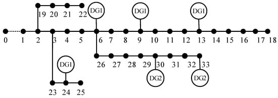
Figure A1.
Distributed power supply configuration of the IEEE 33-node system.
Figure A1.
Distributed power supply configuration of the IEEE 33-node system.

As shown in Table A1, the DG1 active power output of nodes 6, 9, 13, and 24 is 0.5 MW, and the DG2 active power output of nodes 30 and 33 is 0.35 MW and 0.65 MW, respectively.
Table A1.
Parameters of added DGs of 33-bus systems.
Table A1.
Parameters of added DGs of 33-bus systems.
| No. | DG Type | Quantity | Location | Active Power/MW |
|---|---|---|---|---|
| DG1 | PV cell | 1 | 6, 9, 13, 24 | 0~0.5 |
| DG2 | WTG | 1 | 30 | 0~0.35 |
| DG2 | WTG | 1 | 33 | 0~0.65 |
Figure A2 is the schematic diagram of the IEEE 69-node system, and Table A2 shows the distributed power configuration of the IEEE 69-node system.

Figure A2.
Distributed power supply configuration of the IEEE 69-node system.
Figure A2.
Distributed power supply configuration of the IEEE 69-node system.
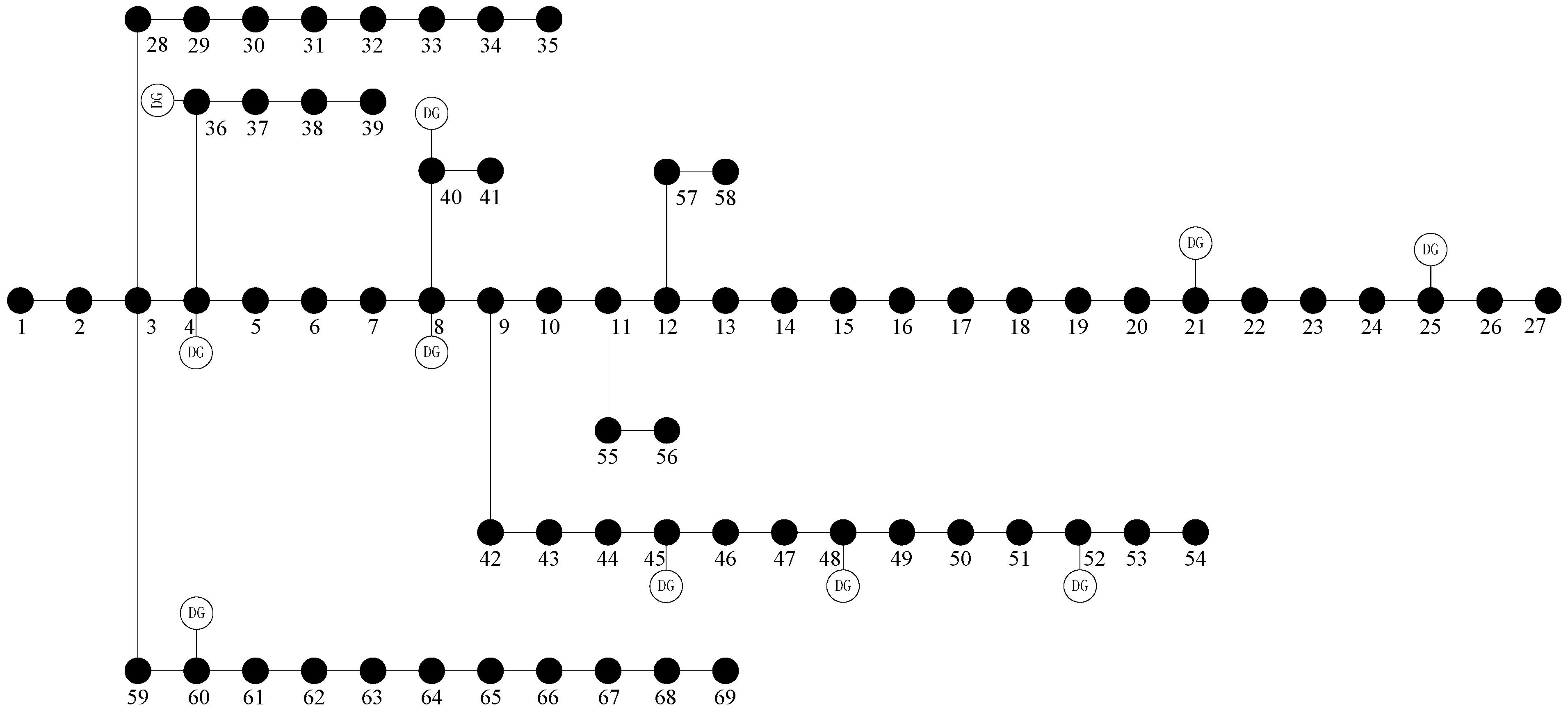
As shown in Table A2, the DG1 active power output of nodes 4, 8, 21, 25, and 36 is 0.35 MW, and the DG2 active power output of nodes 40, 45, 48, 52, and 60 is 0.25 MW.
Table A2.
Parameters of added DGs of 69-bus systems.
Table A2.
Parameters of added DGs of 69-bus systems.
| No. | DG Type | Quantity | Location | Active Power/MW |
|---|---|---|---|---|
| DG1 | PV cell | 1 | 4, 8, 21, 25, 36, | 0~0.35 |
| DG2 | WTG | 1 | 40, 45, 48, 52, 60 | 0~0.25 |
Considering that the distribution area covers a small area, all loads, photovoltaic (PV) cells, and wind turbine (WT) units adopt the same time-series curve, using a typical summer curve of a certain place, as shown in Figure A3.
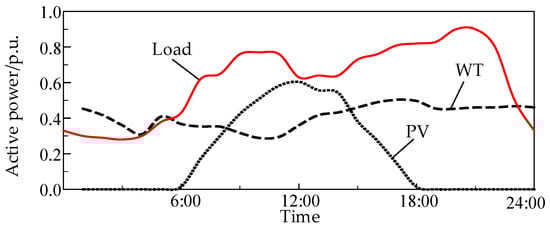
Figure A3.
Daily load curve and daily operation curve of wind turbines and photovoltaic cells.
Figure A3.
Daily load curve and daily operation curve of wind turbines and photovoltaic cells.

References
- Zhang, Z.; Chen, Z. Transformation mechanism and characterization method of multi-agent flexibility and randomness in active distribution Network. Autom. Electr. Power Syst. 2018, 48, 116–129. (In Chinese) [Google Scholar]
- Koutsoukis, N.C.; Georgilakis, P.S.; Hatziargyriou, N.D. Multistage coordinated planning of active distribution networks. IEEE Trans. Power Syst. 2017, 33, 32–44. [Google Scholar] [CrossRef]
- Jiang, X. Feasible Operation Region of an Electricity Distribution Network with SOPs. Ph.D. Thesis, Cardiff University, Cardiff, UK, 2024. [Google Scholar]
- Sun, X.; Qiu, J.; Zhao, J. Optimal Local Volt/Var Control for Photovoltaic Inverters in Active Distribution Networks. IEEE Trans. Power Syst. 2021, 36, 5756–5766. [Google Scholar] [CrossRef]
- Vandoorn, T.L.; Meersman, B.; De Kooning, J.D.M.; Vandevelde, L. Transition From Islanded to Grid-Connected Mode of Microgrids With Voltage-Based Droop Control. IEEE Trans. Power Syst. 2013, 28, 2545–2553. [Google Scholar] [CrossRef]
- Samadi, A.; Eriksson, R.; Söder, L.; Rawn, B.G.; Boemer, J.C. Coordinated Active Power-Dependent Voltage Regulation in Distribution Grids With PV Systems. IEEE Trans. Power Deliv. 2014, 29, 1454–1464. [Google Scholar] [CrossRef]
- Xing, Q.; Chen, Z.; Zhang, T.; Li, X.; Sun, K. Real-time optimal scheduling for active distribution networks: A graph reinforcement learning method. Int. J. Electr. Power Energy Syst. 2023, 145, 108637. [Google Scholar] [CrossRef]
- Xiao, J.; Zu, G.; Bai, G.; Zhang, M.; Wang, C.; Zhao, J. Mathematical Definition and Existence Proof of Security Domain of Distribution System. Proc. CSEE 2016, 36, 4828–4836. (In Chinese) [Google Scholar]
- Xiao, J.; Zuo, L.; Zu, G.; Liu, S. Security Domain Model of Distribution System Based on Power Flow Calculation. Proc. CSEE 2017, 37, 4941–4949. (In Chinese) [Google Scholar]
- Ageeva, L.; Majidi, M.; Pozo, D. Analysis of Feasibility Region of Active Distribution Networks. In Proceedings of the 2019 International Youth Conference on Radio Electronics, Electrical and Power Engineering (REEPE), Moscow, Russia, 14–15 March 2019; pp. 1–5. [Google Scholar]
- Pei, L.; Wei, Z.; Chen, S.; Sun, G.; Lv, S. Security Domain of AC-DC Hybrid Distribution Network based on Convex envelope. Power Syst. Autom. 2021, 45, 45–51. (In Chinese) [Google Scholar]
- Petrou, K.; Procopiou, A.T.; Gutierrez-Lagos, L.; Liu, M.Z.; Ochoa, L.F.; Langstaff, T.; Theunissen, J.M. Ensuring Distribution Network Integrity Using Dynamic Operating Limits for Prosumers. IEEE Trans. Smart Grid 2021, 12, 3877–3888. [Google Scholar] [CrossRef]
- Blackhall, L. On the Calculation and Use of Dynamic Operating Envelopes; Australian National University: Canberra, Australian, 2020. [Google Scholar]
- Liu, B.; Braslavsky, J.H. Sensitivity and robustness issues of operating envelopes in unbalanced distribution networks. IEEE Access 2022, 10, 92789–92798. [Google Scholar] [CrossRef]
- Rayati, M.; Bozorg, M.; Cherkaoui, R.; Carpita, M. Distributionally robust chance constrained optimization for providing flexibility in an active distribution network. IEEE Trans. Smart Grid 2022, 13, 2920–2934. [Google Scholar] [CrossRef]
- Karimianfard, H.; Haghighat, H. Generic resource allocation in distribution grid. IEEE Trans. Power Syst. 2018, 34, 810–813. [Google Scholar] [CrossRef]
- Wang, R.; Ji, H.; Li, P.; Yu, H.; Zhao, J.; Zhao, L.; Zhou, Y.; Wu, J.; Bai, L.; Yan, J.; et al. Multi-resource dynamic coordinated planning of flexible distribution network. Nat. Commun. 2024, 15, 4576. [Google Scholar] [CrossRef] [PubMed]
- Karthikeyan, N.; Pillai, J.R.; Bak-Jensen, B.; Simpson-Porco, J.W. Predictive control of flexible resources for demand response in active distribution networks. IEEE Trans. Power Syst. 2019, 34, 2957–2969. [Google Scholar] [CrossRef]
- Liu, M.Z.; Ochoa, L.F.; Wong, P.K.C.; Theunissen, J. Using opf-based operating envelopes to facilitate residential der services. IEEE Trans. Smart Grid 2022, 13, 4494–4504. [Google Scholar] [CrossRef]
- Bassi, V.; Ochoa, L.N. Deliverables 1-2-3a: Model-Free Voltage Calculations and Operating Envelopes; The University of Melbourne: Melbourne, Australia, 2022. [Google Scholar]
- Chen, X.; Li, N. Leveraging two-stage adaptive robust optimization for power flexibility aggregation. IEEE Trans. Smart Grid 2021, 12, 3954–3965. [Google Scholar] [CrossRef]
- Shi, L.; Xu, X.; Yan, Z.; Tan, Z. Envelop Calculation Method for Active-reactive Power Operation of Distribution Network. Proc. CSEE 2024, 1–15. (In Chinese) [Google Scholar]
- Yang, T.; Yu, Y. Steady-state security region-based voltage/var optimization considering power injection uncertainties in distribution grids. IEEE Trans. Smart Grid 2018, 10, 2904–2911. [Google Scholar] [CrossRef]
- Oladeji, I.; Makolo, P.; Abdillah, M.; Shi, J.; Zamora, R. Security impacts assessment of active distribution network on the modern grid operation—A review. Electronics 2021, 10, 2040. [Google Scholar] [CrossRef]
- Gu, C.; Wang, Y.; Wang, W.; Gao, Y. Research on Load State Sensing and Early Warning Method of Distribution Network under High Penetration Distributed Generation Access. Energies 2023, 16, 3093. [Google Scholar] [CrossRef]
- Hu, D.; Peng, Y.; Wei, W.; Xiao, T.; Cai, T.; Xi, W. Reactive power optimization strategy of deep reinforcement learning for distribution network with multiple time scales. Proc. CSEE 2022, 42, 5034–5045. (In Chinese) [Google Scholar]
- Zhang, J.; Cui, M.; Yao, X.; He, Y. Dual time-scale coordinated optimization of active distribution network based on data-driven and physical model. Automation of Electr. Power Syst. 2023, 47, 64–71. (In Chinese) [Google Scholar]
- Lin, Z.; Hu, Z.; Song, Y. Review of Convex relaxation Techniques for optimal power flow Problems. Proc. CSEE 2019, 39, 3717–3728. [Google Scholar]
- Ju, Y.; Huang, Y.; Zhang, R. Optimal power flow of three-phase AC-DC hybrid active distribution Network based on second-order cone programming convex relaxation. Trans. China Electrotech. Soc. 2021, 36, 1866–1875. (In Chinese) [Google Scholar]
- Heidari, R.; Seron, M.M.; Braslavsky, J.H. Non-local approximation of power flow equations with guaranteed error bounds. In Proceedings of the 2017 Australian and New Zealand Control Conference (ANZCC), Gold Coast, QLD, Australia, 17–20 December 2017; pp. 83–88. [Google Scholar]
- Borghetti, A.; Bosetti, M.; Grillo, S.; Massucco, S.; Nucci, C.A.; Paolone, M.; Silvestro, F. Short-term scheduling and control of active distribution systems with high penetration of renewable resources. IEEE Syst. J. 2010, 4, 313–322. [Google Scholar] [CrossRef]
- Pilo, F.; Pisano, G.; Soma, G.G. Optimal coordination of energy resources with a two-stage online active management. IEEE Trans. Ind. Electron. 2011, 58, 4526–4537. [Google Scholar] [CrossRef]
- Huang, Y.; Wang, Y.; Kong, W.; Cao, C.; Su, J.; Wang, K. Active power and reactive power coordination optimization of active distribution network based on improved convex inner approximation method. Proc. CSEE 2024, 1–11. (In Chinese) [Google Scholar]
- Li, H.; He, H. Learning to operate distribution networks with safe deep reinforcement learning. IEEE Trans. Smart Grid 2022, 13, 1860–1872. [Google Scholar] [CrossRef]
- Kou, P.; Liang, D.; Wang, C.; Wu, Z.; Gao, L. Safe deep reinforcement learning-based constrained optimal control scheme for active distribution networks. Appl. Energy 2020, 264, 114772. [Google Scholar] [CrossRef]
- Mu, Y.; Jin, S.; Zhao, K.; Dong, X.; Jia, H.; Qi, Y. “people-car-pile-road-net” depth under the coupling of the collaborative planning and operation optimization distribution network. Autom. Electr. Power Syst. 2018, 48, 24–37. (In Chinese) [Google Scholar]
- Lu, S.; Mo, Y. Distributed dispatching method of active distribution network considering multiple regulation resources. J. Phys. Conf. Ser. 2022, 2237, 012004. [Google Scholar] [CrossRef]
- Sun, H.; Ding, X.; Wu, Z.; Zheng, S.; Xu, Z. Voltage regulation strategy of distribution network with automatic voltage control system limit optimization. Electr. Power Syst. Autom. 2024, 1–13. (In Chinese) [Google Scholar]
- Guo, Q.; Wu, J.; Mo, C.; Xu, H. Collaborative optimization model of voltage and reactive power for new energy distribution Network based on mixed integer second-order cone programming. Proc. CSEE 2018, 38, 1385–1396. (In Chinese) [Google Scholar]
- Chen, S.; Wei, Z.; Sun, G.; Wei, W.; Wang, D. Convex hull based robust security region for electricity-gas integrated energy systems. IEEE Trans. Power Syst. 2018, 34, 1740–1748. [Google Scholar] [CrossRef]


Disclaimer/Publisher’s Note: The statements, opinions and data contained in all publications are solely those of the individual author(s) and contributor(s) and not of MDPI and/or the editor(s). MDPI and/or the editor(s) disclaim responsibility for any injury to people or property resulting from any ideas, methods, instructions or products referred to in the content. |
© 2024 by the authors. Licensee MDPI, Basel, Switzerland. This article is an open access article distributed under the terms and conditions of the Creative Commons Attribution (CC BY) license (https://creativecommons.org/licenses/by/4.0/).