Current Sensorless Pole-Zero Cancellation Output Voltage Control for Uninterruptible Power Supply Systems with a Three-Phase Inverter

Abstract

This article presents a proportional–derivative (PD) type output voltage regulator without the current feedback, taking into account system parameter and load variations. The main advantages are given as follows: First, the first-order output voltage derivative observer is developed without the requirement of system parameter information, which makes it possible to stabilize the system without current sensing. Second, a simple self-tuner implements the feedback-loop adaptation by updating the desired dynamics accordingly. Third, the observer-based active damping injection for the PD-type controller results in the closed-loop system order reduction to 1 by the pole-zero cancellation, including the disturbance observer as a feed-forward term. The prototype uninterruptible power supply system comprised of a 3 kW three-phase inverter, inductors, and capacitors verifies the practical merits of the proposed technique for linear and nonlinear loads.

1. Introduction

The power conversion between AC and DC is a pivotal task for a wide range of industrial applications, such as home appliances, electric vehicles, factory automation, etc. These applications require of the power converters to secure the high performance in both transient and steady state operations. In particular, the uninterruptible power supply (UPS) systems composed of the three-phase inverter and output $LC$-filter must be carefully designed to meet the specified high-level closed-loop performance under the abrupt power failure scenario (i.e., DC to AC power conversion) [1,2,3,4,5].

The combination of inner-loop current control and outer-loop voltage control has been popularly adopted to regulate the output voltage with its implementation from the proportional–integral (PI) regulator, due to its simple structure and tuning process. The corresponding feedback gains were tuned via the trial-and-error, Zeigler–Nichols, Bode, and Nyquist techniques, conventionally [6,7]. The resultant closed-loop stability and performance were only valid for the fixed operating mode (i.e., given fixed load conditions). The additional gain scheduling mechanism as in [8] successfully enlarged the feasible operating region with an increased computational burden. The feed-forward terms and specific PI gains were introduced with the use of a rotational coordinate transformation to result in the first-order closed-loop transfer functions with desired cut-off frequencies for each loop via pole-zero cancellation (PZC), which required the true system parameters, such as resistance, inductance, and capacitance [9,10]. Novel online identifiers can be used as the solution to the parameter dependence problem [11,12,13]. The deadbeat-type control provides rapid regulation performance, but is sensitive to high measurement noise sensitivity due to its exact model dependence [14]. This practical limitation was systematically handled by the parameter-dependent observer-based deadbeat controllers [15,16]. The optimal state-feedback controls such as $H_{\infty }$ and $\mu$-synthesis techniques solved the output voltage control problem considering the external disturbances from the load failure [17,18]. The sliding-mode technique with the conservative discontinuous sign function provides the stabilization and performance recovery property by ensuring the reaching property to the sliding surface [19]. The model predictive control (MPC) generates the optimal duty command for the three-phase inverter considering the input and state constraints with the requirement of parameter dependence and high computational burden [20,21,22]. To address the computational burden issue, explicit MPC techniques were presented, involving huge offline tasks for partitioning the state space properly; however, this approach could lead to computational burdens from the significant online membership tests [23,24]. To avoid the online optimization and membership tests, the one-step MPC control with full-state feedback was devised, including the disturbance observer (DOB) to replace the regulation error integrators and improving the closed-loop robustness against the load variations [25]. The system parameter, load variations, and one-step time-delay were explicitly considered using a robust-state feedback design technique incorporating regulation error integrators and LMI optimization [26]. Under a similar strategy, the DOB and one-step-ahead state predictor were included for the one-step MPC and finite control set MPC (FCSMPC) as the optimization solution to the output voltage regulation problem with parameter uncertainties [27,28,29]. There are two practical challenges in the previous results, the parameter dependence of controls and state-observers, at least partially, and fixed closed-loop cut-off frequency, to be handled in this study; it is desirable for the cut-off frequency to be decreased in the steady-state and to be increased in the transient periods.

The aforementioned literature survey identifies the following practical challenges that need to be addressed: (P1) performance inconsistency for load variations, (P2) limited current measurement, (P3) fixed closed-loop bandwidth, and (P4) system model dependence. The proposed solution forms the single-loop feedback structure without the current loop, independent of the exact model information for both the observer and controller. The contributions of the proposed technique are summarized as follows.

• For (P2) and (P4): The output voltage derivative observer is built by combining the Luenberger observer and DOB design techniques without requiring the true system parameter information; this eliminates the need of current feedback.
• For (P3): The online self-tuner adjusts the desired dynamics to implement the feedback-loop adaptation according to the transient and steady-state operation modes.
• For (P1) and (P4): The injection of the active damping term and special form of feedback gain for the DOB-based proportional-derivative (PD) controller result in the stable PZC to render the closed-loop system order to be 1.

A prototype 3 kW UPS system was used to experimentally confirm the effectiveness of the proposed technique under the resistive and rectifier loads, deriving from the beneficial closed-loop properties.

There are five sections to organize this paper. Section 2 introduces the servo motor model with the strategy of handling the parameter and load variations. Section 3 describes the design purpose and presents the proposed solution. Section 4 proves the accomplishment of the design purpose by analyzing the closed-loop dynamics. Section 5 experimentally validates the effectiveness of the proposed solution. Section 6 concludes this paper.

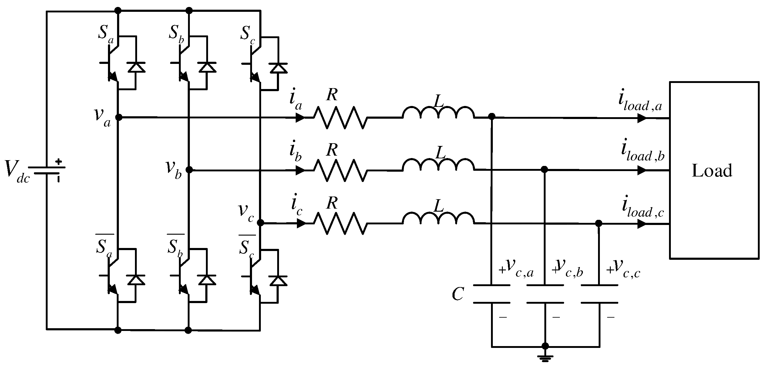
2. Uninterruptible Power Supply System Dynamics

The UPS systems are comprised of a three-phase inverter, inductor, and output capacitor, as shown in Figure 1. The application of Kirchhoff’s voltage law to the UPS systems leads to the linear time-invariant system (LTI):

$$\begin{array}{ccc}\hfill C{\dot{\mathbf{v}}}_{c,abc}& =& {\mathbf{i}}_{abc}-{\mathbf{i}}_{load,abc},\hfill \end{array}$$

(1)

$$\begin{array}{ccc}\hfill L{\dot{\mathbf{i}}}_{abc}& =& {\mathbf{u}}_{abc}-R{\mathbf{i}}_{abc}-{\mathbf{v}}_{c,abc},\forall t\ge 0,\hfill \end{array}$$

(2)

with the inductor current ${\mathbf{i}}_{abc}={\left[\begin{array}{ccc}{i}_a& i_b& i_c\end{array}\right]}^T$, capacitor voltage ${\mathbf{v}}_{c,abc}={\left[\begin{array}{ccc}{v}_{c,a}& v_{c,b}& v_{c,c}\end{array}\right]}^T$, and control signal ${\mathbf{u}}_{abc}={\left[\begin{array}{ccc}{u}_a& u_b& u_c\end{array}\right]}^T$ defined as

$$\begin{array}{ccc}\hfill {\mathbf{u}}_{abc}& =& \frac{1}{6}\left[\begin{array}{ccc}2& -1& -1\\ -1& 2& -1\\ -1& -1& 2\end{array}\right]\left[\begin{array}{c}{p}_a\\ p_b\\ p_c\end{array}\right]V_{dc},\hfill \\ \hfill p_x& =& \left\{\begin{array}{c}1\mathrm{if}{S}_x:\mathrm{ON}\mathrm{and}{\overline{S}}_x:\mathrm{OFF},\\ -1\mathrm{if}{S}_x:\mathrm{OFF}\mathrm{and}{\overline{S}}_x:\mathrm{ON},\end{array}\right.\hfill \end{array}$$

(3)

where $x=a,b,c$. The load current is denoted as ${\mathbf{i}}_{load,abc}={\left[\begin{array}{ccc}{i}_{load,a}& i_{load,b}& i_{load,c}\end{array}\right]}^T$, to be treated as the unknown disturbance due to the load uncertainties. It should be noted that the capacitor voltage reference is normally given by the three-phase balanced form ${\mathbf{v}}_{c,abc,ref}=r{\left[\begin{array}{ccc}cos\left({\omega }_{r}t\right)& cos({\omega }_r-\frac{2\pi }{3})& cos({\omega }_{r}t-\frac{4\pi }{3})\end{array}\right]}^T$ for some $r>0$ and ${\omega }_r=2\pi f$ rad/s.

The alternative system behaviors (1) and (2) make the tracking controller design task difficult. The coordinate transformation defined as

$$\mathbf{W}\left({\theta }_r\right):=\left[\begin{array}{ccc}cos\left({\theta }_r\right)& cos({\theta }_r-\frac{2\pi }{3})& cos({\theta }_r-\frac{4\pi }{3})\\ -sin\left({\theta }_r\right)& -sin({\theta }_r-\frac{2\pi }{3})& -sin({\theta }_r-\frac{4\pi }{3})\end{array}\right],$$

synchronized to the phase angle ${\theta }_r:={\omega }_{r}t$ with desired frequency ${\omega }_r$, eliminates the alternative component of system dynamics as

$$\begin{array}{ccc}\hfill C{\dot{\mathbf{v}}}_c& =& \mathbf{i}+C{\omega }_r\mathbf{J}{\mathbf{v}}_c-{\mathbf{i}}_{load},\hfill \end{array}$$

(4)

$$\begin{array}{ccc}\hfill L\dot{\mathbf{i}}& =& (-R\mathbf{I}+L{\omega }_r\mathbf{J})\mathbf{i}-{\mathbf{v}}_c+\mathbf{u},\forall t\ge 0,\hfill \end{array}$$

(5)

through the calculations resulting in the d-q axis variables $\mathbf{i}=\left[\begin{array}{c}{i}_d\\ i_q\end{array}\right]$, ${\mathbf{v}}_c=\left[\begin{array}{c}{v}_{c,d}\\ v_{c,q}\end{array}\right]$, ${\mathbf{i}}_{load}=\left[\begin{array}{c}{i}_{load,d}\\ i_{load,q}\end{array}\right]$, and $\mathbf{u}=\left[\begin{array}{c}{u}_d\\ u_q\end{array}\right]$, such that

$$\begin{array}{c}\hfill \mathbf{i}=\frac{2}{3}\mathbf{W}\left({\theta }_r\right){\mathbf{i}}_{abc},{\mathbf{v}}_c=\frac{2}{3}\mathbf{W}\left({\theta }_r\right){\mathbf{v}}_{c,abc},{\mathbf{i}}_{load}=\frac{2}{3}\mathbf{W}\left({\theta }_r\right){\mathbf{i}}_{load,abc},and\mathbf{u}=\frac{2}{3}\mathbf{W}\left({\theta }_r\right){\mathbf{u}}_{abc},\end{array}$$

$\forall t\ge 0$. The two symbols $\mathbf{I}$ and $\mathbf{J}$ denote the $2\times 2$-dimensional identity and skew-symmetric matrices, respectively, which are $\mathbf{I}=\left[\begin{array}{cc}1& 0\\ 0& 1\end{array}\right]$ and $\mathbf{J}=\left[\begin{array}{cc}0& 1\\ -1& 0\end{array}\right]$.

The passive component (capacitance and inductance) values C and L can be dramatically changed depending on the magnitude of current and voltage, which are assumed to be unknown, but their nominal values $C_0$ and $L_0$ are available from the manufacturers. To remove the true system parameter dependence, this study introduces the nominal parameters $C_0$ and $L_0$ to systems (4) and (5), yielding the modified system (5) such that

$$\begin{array}{ccc}\hfill C_0{\dot{\mathbf{v}}}_c& =& \mathbf{i}+C_0{\omega }_r\mathbf{J}{\mathbf{v}}_c+{\mathbf{d}}_{v,o},\hfill \end{array}$$

(6)

$$\begin{array}{ccc}\hfill L_0\dot{\mathbf{i}}& =& (-R_0\mathbf{I}+L_0{\omega }_r\mathbf{J})\mathbf{i}-{\mathbf{v}}_c+\mathbf{u}+{\mathbf{d}}_{i,o},\forall t\ge 0,\hfill \end{array}$$

(7)

with the unknown lumped disturbances ${\mathbf{d}}_{v,o}$ and ${\mathbf{d}}_{i,o}$ modeling the parameter and load variations, which are used for the following controller design and closed-loop analysis sections.

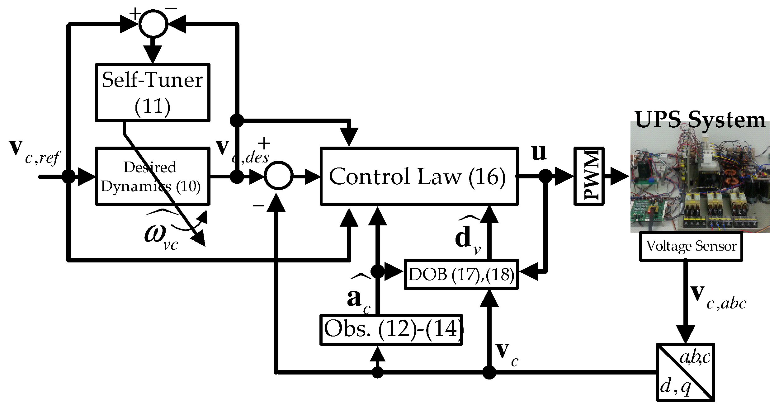
3. Proposed Control Algorithm

The control objective is to render the output voltage ${\mathbf{v}}_c$ to exponentially behave as the target trajectory ${\mathbf{v}}_{c,des,0}={\left[\begin{array}{cc}{v}_{c,d,des,0}& v_{c,q,des,0}\end{array}\right]}^T$, driven by given reference $v_{c,ref}={\left[\begin{array}{cc}{v}_{c,d,ref}& v_{c,q,ref}\end{array}\right]}^T$, satisfying the desired first-order system

$$\begin{array}{c}\hfill {\dot{\mathbf{v}}}_{c,des,0}={\omega }_{v_c}({\mathbf{v}}_{c,ref}-{\mathbf{v}}_{c,des,0}),\forall t\ge 0,\end{array}$$

(8)

with the closed-loop specification ${\omega }_{v_c}>0$ as the convergence rate of system (8). The next subsection presents the self-tuner through a modification of the desired system (8) to implement the feedback-loop adaptation.

Remark 1.

Taking the Laplace transform to desired system (8) (e.g., $V_{c,d,des,0}\left(s\right)=\mathcal{L}\left\{v_{c,d,des,0}\right\}$, $V_{c,q,des,0}\left(s\right)=\mathcal{L}\left\{v_{c,q,des,0}\right\}$, $V_{c,d,ref}\left(s\right)=\mathcal{L}\left\{v_{c,d,ref}\right\}$, and $V_{c,q,ref}\left(s\right)=\mathcal{L}\left\{v_{c,q,ref}\right\}$) derives the transfer function forming the low-pass filter (LPF):

$$\begin{array}{c}\hfill \frac{V_{c,x,des,0}\left(s\right)}{V_{c,x,ref}\left(s\right)}=\frac{{\omega }_{vc}}{s+{\omega }_{vc}},x=d,q,\forall s\in \mathbb{C},\end{array}$$

(9)

with the cut-off frequency ${\omega }_{vc}$ (rad/s, $\frac{{\omega }_{vc}}{2\pi }$ Hz). Therefore, the closed-loop specification ${\omega }_{v_c}$ can be determined as the cut-off frequency of the LPF (9) from the reference to the desired output.

3.1. Self-Tuner

To implement the feedback-loop adaptation, this study slightly modifies the desired system (8) as ${\mathbf{v}}_{c,des}={\mathbf{v}}_{c,des,0}{|}_{{\omega }_{v_c}={\widehat{\omega }}_{v_c}}$, yielding

$$\begin{array}{c}\hfill {\dot{\mathbf{v}}}_{c,des}={\widehat{\omega }}_{v_c}({\mathbf{v}}_{c,ref}-{\mathbf{v}}_{c,des}),\forall t\ge 0,\end{array}$$

(10)

with the proposed self-tuner driving the cut-off frequency ${\widehat{\omega }}_{v_c}$ initiated from ${\widehat{\omega }}_{v_c}\left(0\right)={\omega }_{v_c}$ as

$$\begin{array}{c}\hfill {\dot{\widehat{\omega }}}_{v_c}={\gamma }_{v_c}(\parallel {\tilde{\mathbf{v}}}_{c,des}{\parallel }^2+{\rho }_{v_c}{\tilde{\omega }}_{v_c}),\forall t\ge 0,\end{array}$$

(11)

with errors defined as ${\tilde{\mathbf{v}}}_{c,des}:={\mathbf{v}}_{c,ref}-{\mathbf{v}}_{c,des}$, and ${\tilde{\omega }}_{v_c}:={\omega }_{v_c}-{\widehat{\omega }}_{v_c}$ and tuning factors ${\gamma }_{v_c}>0$ and ${\rho }_{v_c}>0$. The self-tuner (11) automatically adjusts the cut-off frequency ${\widehat{\omega }}_{v_c}$ to increase the error decay ratio of ${\tilde{\mathbf{v}}}_{c,des}$ with the boundedness property of ${\widehat{\omega }}_{v_c}\ge {\omega }_{v_c}$, $\forall t\ge 0$. For details, see Section 4. The next issue is designing an observer for the output voltage derivative, which makes it available to inject the active damping term and to feedback the regulation error derivatives.

3.2. Observer

It is undesirable to apply the time derivative operation to the output voltage measurement ${\mathbf{v}}_c$ to make the signal ${\mathbf{a}}_c:={\dot{\mathbf{v}}}_c$ available for feedback, due to the high-frequency measurement noise. To avoid this problem and system parameter dependence, the observer for ${\mathbf{a}}_c$ is proposed as

$$\begin{array}{ccc}\hfill {\dot{\widehat{\mathbf{v}}}}_c& =& k_{obs}{\mathbf{e}}_{v_c}+{\widehat{\mathbf{a}}}_c,\hfill \end{array}$$

(12)

$$\begin{array}{ccc}\hfill {\dot{\mathbf{z}}}_{a_c}& =& -l_{a_c}{\mathbf{z}}_{a_c}-l_{a_c}^2{\mathbf{e}}_{v_c}+l_{a_c}({\widehat{\mathbf{a}}}_c+k_{obs}{\mathbf{e}}_{v_c}),\hfill \end{array}$$

(13)

$$\begin{array}{ccc}\hfill {\widehat{\mathbf{a}}}_c& =& {\mathbf{z}}_{a_c}+l_{a_c}{\mathbf{e}}_{v_c},\forall t\ge 0,\hfill \end{array}$$

(14)

with the estimation error ${\mathbf{e}}_{v_c}:={\mathbf{v}}_c-{\widehat{\mathbf{v}}}_c$ and observer gains $k_{obs}>0$ and $l_{a_c}>0$. The proposed observer of (12)–(14) drives the estimate ${\widehat{\mathbf{a}}}_c$ to tend to their actual measurement of ${\dot{\mathbf{v}}}_c$, exponentially, without any use of plant parameters, which corresponds to a feature of this study, unlike the conventional Luenberger observers. The first part (12) is devised by the standard Luenberger observer design technique for the plant dynamics ${\dot{\mathbf{v}}}_c={\mathbf{a}}_c$. The remaining parts (13) and (14) come from the DOB design technique using the observer error dynamics for (12). The estimation error convergence property is provided in Section 4.

3.3. Control Law

To remove the current-loop dependence, this study applies the additional derivative to system (6) to obtain the second-order open-loop system given by

$$\begin{array}{ccc}\hfill L_0{C}_0{\ddot{\mathbf{v}}}_c& =& L_0\dot{\mathbf{i}}+L_0{C}_0{\omega }_r\mathbf{J}{\dot{\mathbf{v}}}_c+L_0{\dot{\mathbf{d}}}_{v,o}\hfill \\ & =& (L_0{C}_0{\omega }_r^2{\mathbf{J}}^2-\mathbf{I}){\mathbf{v}}_c+\mathbf{u}+{\mathbf{d}}_v,\forall t\ge 0,\hfill \end{array}$$

(15)

with the lumped disturbance defined as ${\mathbf{d}}_v:=L_0{\omega }_r\mathbf{J}(\mathbf{i}+{\mathbf{d}}_{v,o})+(-R_0\mathbf{I}+L_0{\omega }_r\mathbf{J})\mathbf{i}+{\mathbf{d}}_{i,o}+L_0{\dot{\mathbf{d}}}_{v,o}$, where the current dynamics (7) is used for the second equation above. Due to the unavailability of voltage derivative, the observer-based PD-type control law is proposed by involving the estimated variable ${\widehat{\mathbf{a}}}_c$, such that

$$\begin{array}{c}\hfill \mathbf{u}=-k_{vc}{\widehat{\mathbf{a}}}_c+L_0{C}_0{\lambda }_{vc}({\dot{\mathbf{v}}}_{c,des}-{\widehat{\mathbf{a}}}_c)+k_{vc}{\lambda }_{vc}{\tilde{\mathbf{v}}}_c-{\widehat{\mathbf{d}}}_v-(L_0{C}_0{\omega }_r^2{\mathbf{J}}^2-\mathbf{I}){\mathbf{v}}_c,\forall t\ge 0,\end{array}$$

(16)

for the error ${\tilde{\mathbf{v}}}_c:={\mathbf{v}}_{c,des}-{\mathbf{v}}_c$, active damping coefficient $k_{vc}>0$, feedback gain ${\lambda }_{vc}>0$, and observer-based DOB are given by

$$\begin{array}{ccc}\hfill {\dot{\mathbf{z}}}_v& =& -l_v{\mathbf{z}}_v-l_v^2{L}_0{C}_0{\widehat{\mathbf{a}}}_c-l_v((L_0{C}_0{\omega }_r^2{\mathbf{J}}^2-\mathbf{I}){\mathbf{v}}_c+\mathbf{u}),\hfill \end{array}$$

(17)

$$\begin{array}{ccc}\hfill {\widehat{\mathbf{d}}}_v& =& {\mathbf{z}}_v+l_v{L}_0{C}_0{\widehat{\mathbf{a}}}_c,\forall t\ge 0,\hfill \end{array}$$

(18)

with the gain $l_v>0$. It should be noted that the DOB (17) and (18) ensures the convergence of ${\widehat{\mathbf{d}}}_{\infty }\to {\mathbf{d}}_{\infty }$ (${lim}_{t\to \infty }\mathbf{f}={\mathbf{f}}_{\infty }$ for any function $\mathbf{f}$), and that the combination of active damping coefficient $k_{vc}$ and PD gains $k_{vc}{\omega }_{vc}$ and $L_0{C}_0{\omega }_{vc}$ results in the closed-loop system order reduction to 1 by the PZC. For details, see Section 4. Figure 2 shows the control system structure.

4. Analysis

This section proves that the proposed control system depicted in Figure 2 accomplishes the control objective (10) without offset errors, by ensuring the performance recovery property. First, Section 4.1 derives the properties of proposed self-tuner (11) to make the closed-loop analysis process simple.

4.1. Self-Tuner

The stability of the desired system (10) remains questionable due to the time-varying nature of ${\widehat{\omega }}_{vc}$ driven by the self-tuner (11). Lemma 1 addresses this issue by analyzing the two dynamics (10) and (11).

Lemma 1.

The cut-off frequency ${\widehat{\omega }}_{v_c}$ from the proposed self-tuner (11) ensures that

$$\begin{array}{c}\hfill \underset{t\to \infty }{lim}{\mathbf{v}}_{c,des}={\mathbf{v}}_{c,ref},\end{array}$$

as ${\dot{\mathbf{v}}}_{c,ref}\to \mathbf{0}$ exponentially.

Proof. 

The error ${\tilde{\mathbf{v}}}_{c,des}={\mathbf{v}}_{c,ref}-{\mathbf{v}}_{c,des}$ yields that

$$\begin{array}{c}\hfill {\dot{\tilde{\mathbf{v}}}}_{c,des}=-{\omega }_{v_c}{\tilde{\mathbf{v}}}_{c,des}+{\tilde{\omega }}_{v_c}{\tilde{\mathbf{v}}}_{c,des}+{\dot{\mathbf{v}}}_{c,ref},\forall t\ge 0,\end{array}$$

(19)

using (10). Then, the time derivative of $V_{st}$ defined by

$$\begin{array}{c}\hfill V_{st}=\frac{1}{2}{\parallel {\tilde{\mathbf{v}}}_{c,des}\parallel }^2+\frac{1}{2{\gamma }_{v_c}}{\tilde{\omega }}_{v_c}^2,\forall t\ge 0,\end{array}$$

(20)

is obtained as

$$\begin{array}{ccc}\hfill {\dot{V}}_{st}& =& {\tilde{\mathbf{v}}}_{c,des}^T(-{\omega }_{vc}{\tilde{\mathbf{v}}}_{c,des}+{\tilde{\omega }}_{vc}{\tilde{\mathbf{v}}}_{c,des}+{\dot{\mathbf{v}}}_{c,ref})-{\tilde{\omega }}_{v_c}(\parallel {\tilde{\mathbf{v}}}_{c,des}{\parallel }^2+{\rho }_{v_c}{\tilde{\omega }}_{vc})\hfill \\ & =& -{\omega }_{v_c}{\parallel {\tilde{\mathbf{v}}}_{c,des}\parallel }^2-{\rho }_{v_c}{\tilde{\omega }}_{vc}^2+{\dot{\mathbf{v}}}_{c,ref}^T{\tilde{\mathbf{v}}}_{c,des},\hfill \\ & \le & -{\alpha }_{st}{V}_{st}+{\dot{\mathbf{v}}}_{c,ref}^T{\tilde{\mathbf{v}}}_{c,des},\forall t\ge 0,\hfill \end{array}$$

(21)

with the positive coefficient defined as ${\alpha }_{st}:=min\{2{\omega }_{v_c},2{\gamma }_{v_c}{\rho }_{v_c}\}$, which confirms the result of this theorem, since the strict passivity of ${\dot{\mathbf{v}}}_{c,ref}\mapsto {\tilde{\mathbf{v}}}_{c,des}$, as shown in (21), implies the ${\mathcal{L}}_2$-stability for the same mapping [30]. □

Lemma 2 asserts that the proposed self-tuner (11) renders the convergence rate of the desired system (10) higher than its original version (8), by ensuring the existence of a lower bound of the time-varying gain ${\widehat{\omega }}_{vc}$.

Lemma 2.

The cut-off frequency ${\widehat{\omega }}_{v_c}$ adjusted by self-tuner (11) is bounded below by its initial value ${\omega }_{v_c}$ for all time, i.e., ${\widehat{\omega }}_{v_c}\ge {\omega }_{v_c}$, $\forall t\ge 0$.

Proof. 

The proposed self-tuner (11) can be written as follows in the form of an LTI system:

$$\begin{array}{c}\hfill {\dot{\widehat{\omega }}}_{v_c}=-{\gamma }_{v_c}{\rho }_{v_c}{\widehat{\omega }}_{v_c}+{\gamma }_{v_c}{\rho }_{v_c}{\omega }_{v_c}+{\gamma }_{v_c}{\parallel {\tilde{\mathbf{v}}}_{c,des}\parallel }^2,\forall t\ge 0,\end{array}$$

whose equivalent form is obtained by the integration of both sides as

$$\begin{array}{ccc}\hfill {\widehat{\omega }}_{v_c}& =& e^{-{\gamma }_{v_c}{\rho }_{v_c}t}{\omega }_{v_c}+{\int }_0^t{e}^{-{\gamma }_{v_c}{\rho }_{v_c}(t-\tau )}({\gamma }_{v_c}{\rho }_{v_c}{\omega }_{v_c}+{\gamma }_{v_c}\parallel {\tilde{\mathbf{v}}}_{c,des}{\parallel }^2)d\tau \hfill \\ & \ge & {\omega }_{v_c},\forall t\ge 0.\hfill \end{array}$$

This completes the proof. □

The inequality (21) is useful to prove the performance recovery property in Theorem 1 as the main result of this section. Lemma 3 derives the state estimation behavior by investigating the observer implementation of (12)–(14).

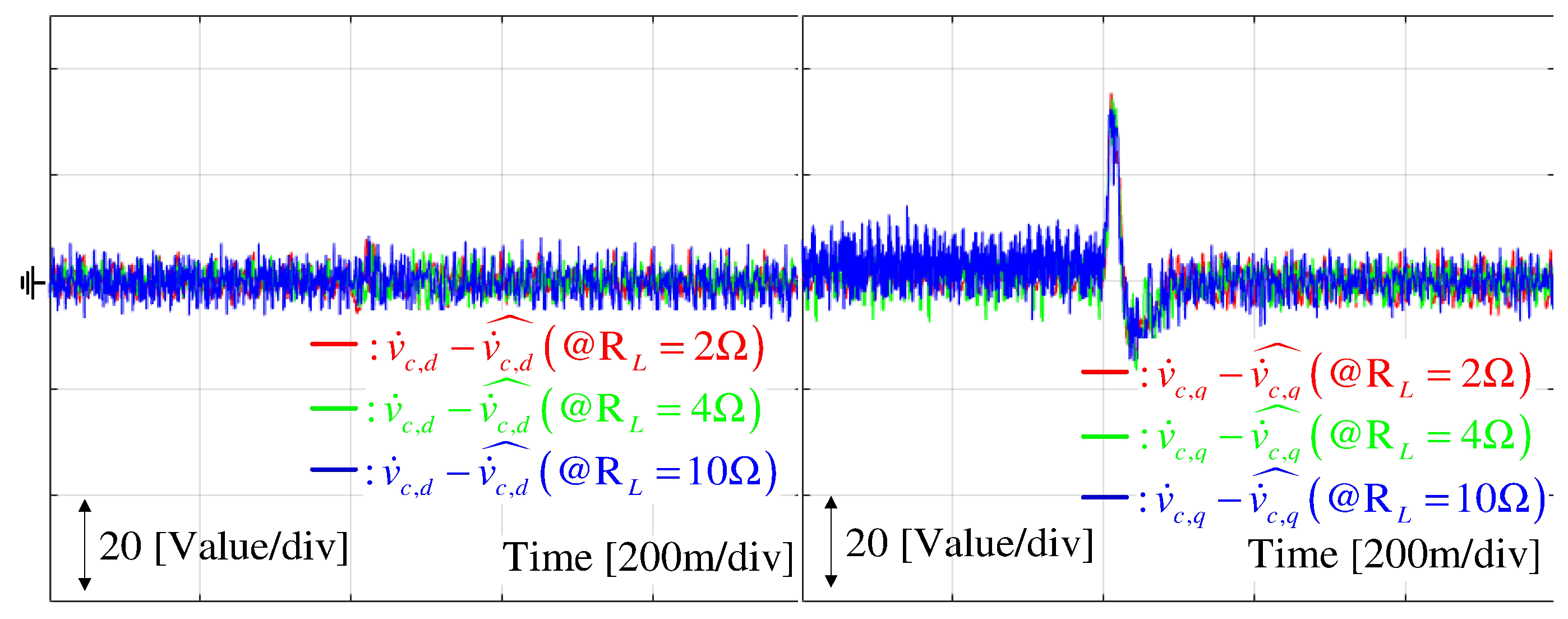
4.2. Observer and DOB

It is easily seen that the filtering error ${\mathbf{e}}_{v_c}={\mathbf{v}}_c-{\widehat{\mathbf{v}}}_c$ gives the dynamics using (12) as

$$\begin{array}{c}\hfill {\dot{\mathbf{e}}}_{v_c}=-k_{obs}{\mathbf{e}}_{v_c}+{\mathbf{e}}_{a_c},\forall t\ge 0,\end{array}$$

(22)

with estimation error ${\mathbf{e}}_{a_c}:={\mathbf{a}}_c-{\widehat{\mathbf{a}}}_c$, which is obvious due to the Luenberger observer form of (12). The estimation error dynamics (22) make it possible to show the acceleration estimation error dynamics in the first-order LPF form.

Lemma 3.

The proposed observer of (12)–(14) yields the following first-order state estimation behaviors:

$$\begin{array}{c}\hfill {\dot{\widehat{\mathit{a}}}}_c=l_{a_c}({\mathit{a}}_c-{\widehat{\mathit{a}}}_c),\forall t\ge 0.\end{array}$$

(23)

Proof. 

The observer output (14) gives the dynamics as

$$\begin{array}{c}\hfill {\dot{\widehat{\mathbf{a}}}}_c=-l_{a_c}({\widehat{\mathbf{a}}}_c-l_{a_c}{\mathbf{e}}_{v_c})-l_{a_c}^2{\mathbf{e}}_{v_c}+l_{a_c}({\widehat{\mathbf{a}}}_c+k_{obs}{\mathbf{e}}_{v_c})+l_{a_c}{\dot{\mathbf{e}}}_{v_c},\forall t\ge 0,\end{array}$$

using the observer dynamics (13), which can be written as

$$\begin{array}{c}\hfill {\dot{\widehat{\mathbf{a}}}}_c=l_{a_c}({\dot{\mathbf{e}}}_{v_c}+k_{obs}{\mathbf{e}}_{v_c})=l_{a_c}{\mathbf{e}}_{a_c},\forall t\ge 0,\end{array}$$

with the application of (22), which completes the proof. □

The estimation error ${\tilde{\mathbf{a}}}_c={\mathbf{a}}_c-{\widehat{\mathbf{a}}}_c$ satisfies that ${\dot{\mathbf{e}}}_{a_c}=-l_{a_c}{\mathbf{e}}_{a_c}+{\dot{\mathbf{a}}}_c$ because of (23), which implies that ${\dot{\mathbf{e}}}_{a_c}=-l_{a_c}{\mathbf{e}}_{a_c}$ as $l_{a_c}\to \infty$. Therefore, it is reasonable to assume that

$$\begin{array}{c}\hfill {\dot{\mathbf{e}}}_{a_c}=-l_{a_c}{\mathbf{e}}_{a_c},\forall t\ge 0,\end{array}$$

(24)

for a sufficiently large value of $l_{a_c}>0$.

Lemma 4 shows the estimated disturbance behavior from the DOBs, which helps for the proof of performance recovery to be considerably simple with the use of Lemma 3.

Lemma 4. 

The DOB of (17) and (18) yields the first-order disturbance estimation behavior:

$$\begin{array}{c}\hfill {\dot{\widehat{\mathit{d}}}}_v=l_v({\mathit{d}}_v-{\widehat{\mathit{d}}}_v)+l_v{l}_{a_c}{L}_0{C}_0{\mathbf{e}}_{a_c},\forall t\ge 0.\end{array}$$

(25)

Proof. 

The differentiation on (18) gives

$$\begin{array}{ccc}\hfill {\dot{\widehat{\mathbf{d}}}}_v& =& {\dot{\mathbf{z}}}_v+l_v{L}_0{C}_0{\dot{\widehat{\mathbf{a}}}}_c\hfill \\ & =& -l_v({\widehat{\mathbf{d}}}_v-l_v{L}_0{C}_0{\widehat{\mathbf{a}}}_c)-l_v^2{L}_0{C}_0{\widehat{\mathbf{a}}}_c-l_v((L_0{C}_0{\omega }_r^2{\mathbf{J}}^2-\mathbf{I}){\mathbf{v}}_c+\mathbf{u})+l_v{L}_0{C}_0{\dot{\mathbf{a}}}_c\hfill \\ & & -l_v{L}_0{C}_0{\dot{\mathbf{e}}}_{a_c}\hfill \\ & =& l_v({\mathbf{d}}_v-{\widehat{\mathbf{d}}}_v)+l_v{l}_{a_c}{L}_0{C}_0{\mathbf{e}}_{a_c},\forall t\ge 0,\hfill \end{array}$$

with the utilization of (17), (18), and (24) for the second and third equations above, sequentially, which completes the proof. □

Defining the disturbance estimation error ${\mathbf{e}}_{d_v}:={\mathbf{d}}_v-{\widehat{\mathbf{d}}}_v$, it holds that ${\dot{\mathbf{e}}}_{d_v}=-l_v{\mathbf{e}}_{d_v}+l_v{l}_{a_c}{L}_0{C}_0{\mathbf{e}}_{a_c}+{\dot{\mathbf{d}}}_v$ because of (25), which implies that ${\dot{\mathbf{e}}}_{d_v}=-l_v{\mathbf{e}}_{d_v}+l_v{l}_{a_c}{L}_0{C}_0{\mathbf{e}}_{a_c}$ as $l_v\to \infty$. Therefore, it is reasonable to assume that

$$\begin{array}{c}\hfill {\dot{\mathbf{e}}}_{d_v}=-l_v{\mathbf{e}}_{d_v}+l_v{l}_{a_c}{L}_0{C}_0{\mathbf{e}}_{a_c},\forall t\ge 0,\end{array}$$

(26)

for a sufficiently large value of $l_v>0$. The two results, (24) and (26), can be compactly written as

$$\begin{array}{c}\hfill \dot{\mathbf{e}}={\mathbf{A}}_e\mathbf{e},\forall t\ge 0,\end{array}$$

(27)

with $\mathbf{e}:={\left[\begin{array}{cc}{\mathbf{e}}_{d_v}^T& {\mathbf{e}}_{a_c}^T\end{array}\right]}^T$ and stable matrix ${\mathbf{A}}_e:=\left[\begin{array}{cc}-l_v{\mathbf{I}}_{2\times 2}& l_v{l}_{a_c}{L}_0{C}_0{\mathbf{I}}_{2\times 2}\\ {\mathbf{0}}_{2\times 2}& -l_{a_c}{\mathbf{I}}_{2\times 2}\end{array}\right]$, which is used for the following analysis.

Remark 2.

Assuming ${\mathit{e}}_{a_c}\approx \mathit{0}$ by result (27), the Laplace transform to the system (25) (e.g., ${\widehat{D}}_{v,d}\left(s\right)=\mathcal{L}\left\{d_{v,d}\right\}$, ${\widehat{D}}_{v,q}\left(s\right)=\mathcal{L}\left\{{\widehat{d}}_{v,q}\right\}$, $D_{v,d}\left(s\right)=\mathcal{L}\left\{d_{v,d}\right\}$, and $D_{v,q}\left(s\right)=\mathcal{L}\left\{d_{v,q}\right\}$) derives the transfer function forming the following low-pass filter (LPF):

$$\begin{array}{c}\hfill \frac{{\widehat{D}}_{v,x}\left(s\right)}{D_{v,x}\left(s\right)}=\frac{l_v}{s+l_v},x=d,q,\forall s\in \mathbb{C},\end{array}$$

(28)

with the cut-off frequency $l_v$ (rad/s, $\frac{l_v}{2\pi }$ Hz). Therefore, the DOB gain $l_v$ can be determined as the cut-off frequency of the LPF (28) from the disturbance to its estimate.

4.3. Control Loop

The combination of active damping and specific form of PD gain occurs in the closed-loop system order reduction to 1 by the stable PZC, which is asserted in Lemma 5.

Lemma 5.

The proposed control law (16) forces the output voltage dynamics to be governed by

$$\begin{array}{c}\hfill {\dot{\mathit{v}}}_c={\lambda }_{v_c}{\tilde{\mathit{v}}}_c+{\mathit{B}}_{e,F}{\mathit{e}}_F,\end{array}$$

(29)

with

$$\begin{array}{c}\hfill {\dot{\mathit{e}}}_F=-a_{e_F}{\mathit{e}}_F+{\mathit{B}}_e\mathit{e},\forall t\ge 0,\end{array}$$

(30)

where $a_{e_F}:=\frac{k_{vc}}{L_0{C}_0}$, ${\mathit{B}}_{e,F}:=\left[\begin{array}{cc}{\mathit{I}}_{2\times 2}& {\mathit{I}}_{2\times 2}\end{array}\right]$, and ${\mathit{e}}_F:={\left[\begin{array}{cc}{\mathit{e}}_{d_v,F}^T& {\mathit{e}}_{a_c,F}^T\end{array}\right]}^T$ for some ${\mathit{B}}_e\in {\mathbb{R}}^{4\times 4}$.

Proof. 

The substitution of (16) to (15) gives the following closed-loop voltage dynamics:

$$\begin{array}{ccc}\hfill L_0{C}_0{\ddot{\mathbf{v}}}_c& =& -k_{vc}{\widehat{\mathbf{a}}}_c+L_0{C}_0{\lambda }_{vc}({\dot{\mathbf{v}}}_{c,des}-{\widehat{\mathbf{a}}}_c)+k_{vc}{\lambda }_{vc}{\tilde{\mathbf{v}}}_c+{\mathbf{e}}_{d_v},\hfill \\ & =& -k_{vc}{\dot{\mathbf{v}}}_c+L_0{C}_0{\lambda }_{vc}{\dot{\tilde{\mathbf{v}}}}_c+k_{vc}{\lambda }_{vc}{\tilde{\mathbf{v}}}_c+{\mathbf{e}}_{d_v}+(k_{vc}+L_0{C}_0{\lambda }_{vc}){\mathbf{e}}_{a_c},\forall t\ge 0.\hfill \end{array}$$

Taking the Laplace transform to both sides above, it follows that

$$\begin{array}{ccc}\hfill (L_0{C}_0{s}^2+(k_{vc}+L_0{C}_0{\lambda }_{vc})s+k_{vc}{\lambda }_{vc}){\mathbf{V}}_c\left(s\right)& =& {\lambda }_{vc}(L_0{C}_{0}s+k_{vc}){\mathbf{V}}_{c,des}\left(s\right)+{\mathbf{E}}_{d_v}\left(s\right)\hfill \\ & & +(k_{vc}+L_0{C}_0{\lambda }_{vc}){\mathbf{E}}_{a_c}\left(s\right),\hfill \end{array}$$

which shows that

$$\begin{array}{c}\hfill (s+{\lambda }_{vc}){\mathbf{V}}_c\left(s\right)={\lambda }_{vc}{\mathbf{V}}_{c,des}\left(s\right)+{\mathbf{E}}_{d_v,F}\left(s\right)+{\mathbf{E}}_{a_c,F}\left(s\right),\forall s\in \mathbb{C},\end{array}$$

due to the PZC by the factorization $(L_0{C}_0{s}^2+(k_{vc}+L_0{C}_0{\lambda }_{vc})s+k_{vc}{\lambda }_{vc})=(L_0{C}_{0}s+k_{vc})(s+{\lambda }_{vc})$, where ${\mathbf{E}}_{d_v,F}\left(s\right)=\frac{\frac{1}{L_0{C}_0}}{s+\frac{k_{vc}}{L_0{C}_0}}$ and ${\mathbf{E}}_{a_c,F}=\frac{\frac{k_{vc}+L_0{C}_0{\lambda }_{vc}}{L_0{C}_0}}{s+\frac{k_{vc}}{L_0{C}_0}}{\mathbf{E}}_{a_c}\left(s\right)$. The application of the inverse Laplace transform to both sides above verifies the result of (29) and (30). □

The performance recovery property, as a main result, can be easily proven by the Lyapunov analysis thanks to the results of Lemmas 3–5.

Theorem 1.

The closed-loop system driven by the proposed control law depicted in Figure 2 guarantees that

$$\begin{array}{c}\hfill \underset{t\to \infty }{lim}{\mathit{v}}_c={\mathit{v}}_{c,des},\end{array}$$

as ${\dot{\mathit{v}}}_{c,ref}\to \mathit{0}$ exponentially.

Proof. 

Let us consider the error dynamics from ${\tilde{\mathbf{v}}}_c={\mathbf{v}}_{c,des}-{\mathbf{v}}_c$ as

$$\begin{array}{ccc}\hfill {\dot{\tilde{\mathbf{v}}}}_c& =& {\dot{\mathbf{v}}}_{c,des}+{\dot{\mathbf{v}}}_c\hfill \\ & =& -{\lambda }_{v_c}{\tilde{\mathbf{v}}}_c-{\mathbf{B}}_{e,F}{\mathbf{e}}_F+{\widehat{\omega }}_{v_c}{\tilde{\mathbf{v}}}_{c,des},\forall t\ge 0,\hfill \end{array}$$

(31)

with the applications of (11) and (29). The combination of (27), (30), and (31) gives the perturbed linear system

$$\begin{array}{c}\hfill {\dot{\mathbf{x}}}_{cl}={\mathbf{A}}_{cl}{\mathbf{x}}_{cl}+{\mathbf{B}}_{cl}{\widehat{\omega }}_{v_c}{\tilde{\mathbf{v}}}_{c,des},\end{array}$$

(32)

with ${\mathbf{x}}_{cl}:={\left[\begin{array}{ccc}{\tilde{\mathbf{v}}}_c^T& {\mathbf{e}}_F^T& {\mathbf{e}}^T\end{array}\right]}^T$, ${\mathbf{B}}_{cl}:={\left[\begin{array}{cc}{\mathbf{I}}_{2\times 2}& {\mathbf{0}}_{2\times 4}\end{array}\right]}^T$, and stable matrix ${\mathbf{A}}_{cl}$ defined as

$$\begin{array}{c}\hfill {\mathbf{A}}_{cl}:=\left[\begin{array}{ccc}-{\lambda }_{v_c}{\mathbf{I}}_{2\times 2}& -{\mathbf{B}}_{e,F}& {\mathbf{0}}_{2\times 4}\\ {\mathbf{0}}_{4\times 2}& -a_1{\mathbf{I}}_{4\times 4}& {\mathbf{B}}_e\\ {\mathbf{0}}_{4\times 2}& {\mathbf{0}}_{4\times 4}& {\mathbf{A}}_e\end{array}\right].\end{array}$$

The stability of matrix ${\mathbf{A}}_{cl}$ makes it solvable for the matrix equation of ${\mathbf{A}}_{cl}^T\mathbf{P}+\mathbf{P}{\mathbf{A}}_{cl}=-\mathbf{I}$ with a unique solution $\mathbf{P}={\mathbf{P}}^T>\mathbf{0}$. The solution $\mathbf{P}>\mathbf{0}$ defines the positive–definite function as

$$\begin{array}{c}\hfill V:=\frac{1}{2}{\mathbf{x}}_{cl}^T\mathbf{P}{\mathbf{x}}_{cl}+\frac{\kappa }{2}{V}_{st},\kappa >0,\forall t\ge 0,\end{array}$$

(33)

with the positive–definite function $V_{st}$ given in (20), whose time derivative is obtained using (21) and (32), and Young’s inequality (e.g., ${\mathbf{x}}^T\mathbf{y}\le \frac{ϵ}{2}{\parallel \mathbf{x}\parallel }^2+\frac{1}{2ϵ}{\parallel \mathbf{y}\parallel }^2$, $\forall \mathbf{x},\mathbf{y}\in {\mathbb{R}}^n$, $\forall ϵ>0$) as

$$\begin{array}{ccc}\hfill \dot{V}& =& -\parallel {\mathbf{x}}_{cl}{\parallel }^2+{\mathbf{x}}_{cl}^T\mathbf{P}{\mathbf{B}}_{cl}{\widehat{\omega }}_{v_c}{\tilde{\mathbf{v}}}_{c,des}-\kappa {\alpha }_{st}{V}_{st}+\kappa {\dot{\mathbf{v}}}_{c,ref}^T{\tilde{\mathbf{v}}}_{c,des}\hfill \\ & \le & -\frac{1}{2}\parallel {\mathbf{x}}_{cl}{\parallel }^2-(\kappa {\alpha }_{st}-{\parallel \mathbf{P}\parallel }^2\parallel {\mathbf{B}}_{cl}{\parallel }^2{\overline{\omega }}_{v_c}^2)V_{st}+\kappa {\dot{\mathbf{v}}}_{c,ref}^T{\tilde{\mathbf{v}}}_{c,des},\forall t\ge 0,\hfill \end{array}$$

with $|{\widehat{\omega }}_{v_c}|\le {\overline{\omega }}_{v_c}$. The constant $\kappa =\frac{1}{{\alpha }_{st}}{(\parallel \mathbf{P}\parallel }^2\parallel {\mathbf{B}}_{cl}{\parallel }^2{\overline{\omega }}_{v_c}^2+\frac{1}{2})$ eliminates the indefinite term so that $\dot{V}$ satisfies

$$\begin{array}{ccc}\hfill \dot{V}& \le & -\frac{1}{2}{\parallel {\mathbf{x}}_{cl}\parallel }^2-\frac{1}{2}{V}_{st}+\kappa {\dot{\mathbf{v}}}_{c,ref}^T{\tilde{\mathbf{v}}}_{c,des}\hfill \\ & \le & -{\alpha }_{cl}V+\kappa {\dot{\mathbf{v}}}_{c,ref}^T{\tilde{\mathbf{v}}}_{c,des},\forall t\ge 0,\hfill \end{array}$$

with ${\alpha }_{cl}:=min\{\frac{1}{{\lambda }_{min}\left(\mathbf{P}\right)},\frac{1}{\kappa }\}$, which concludes that ${\mathbf{x}}_{cl}\to \mathbf{0}$ as ${\dot{\mathbf{v}}}_{c,ref}\to \mathbf{0}$ exponentially. This completes the proof. □

The proposed PD-type controller shown in Figure 2 does not incorporate any integral action, which may suffer from the offset errors in the actual implementations. The DOB as a feed-forward compensation term makes it possible to remove the offset errors in the absence of regulation error integrators, which are addressed in Theorem 2 as another main result of this study.

Theorem 2.

The proposed control law consisting of (12)–(14) and (16)–(18) guarantees ${\mathit{v}}_{c,\infty }={\mathit{v}}_{c,ref,\infty }$ in the actual implementations, where ${\mathit{f}}_{\infty }$ denotes the steady-state value of $\mathit{f}$ for any convergent function $\mathit{f}$.

Proof. 

The closed-loop dynamics of (23), (25), and (29)–(30) result in the steady-state equations

$$\begin{array}{ccc}\hfill \mathbf{0}& =& l_{a_c}{\mathbf{e}}_{a_c,\infty },\hfill \\ \hfill \mathbf{0}& =& l_v{\mathbf{e}}_{d_v,\infty }+l_v{l}_{a_c}{L}_0{C}_0{\mathbf{e}}_{a_c,\infty },\hfill \\ \hfill \mathbf{0}& =& -a_1{\mathbf{e}}_{d_v,F,\infty }+a_2{\mathbf{e}}_{d_v,\infty },\hfill \\ \hfill \mathbf{0}& =& -a_1{\mathbf{e}}_{a_c,F,\infty }+a_3{\mathbf{e}}_{a_c,\infty },\hfill \\ \hfill \mathbf{0}& =& {\lambda }_{v_c}{\tilde{\mathbf{v}}}_{c,\infty }+{\mathbf{e}}_{d_v,F,\infty }+{\mathbf{e}}_{a_c,F,\infty },\hfill \end{array}$$

which show that ${\tilde{\mathbf{v}}}_{c,\infty }=\mathbf{0}$ is equivalent to ${\mathbf{v}}_{c,\infty }={\mathbf{v}}_{c,des,\infty }={\mathbf{v}}_{c,ref,\infty }$, due to the steady-state equation of self-tuner $\mathbf{0}={\widehat{\omega }}_{v_c,\infty }{\tilde{\mathbf{v}}}_{c,des,\infty }$ obtained from (10). Therefore, the claim is true. □

Remark 3. 

The closed-loop analysis results in this section reveal a design parameter tuning process as follows:

• Observer:
  • (Lemma 3) Choose $l_{a_c}$ and $k_{obs}$ such that $l_{a_c}>>k_{obs}$ satisfies the desired observer error dynamics ${\dot{\mathit{e}}}_{a_c}=-l_{a_c}{\mathit{e}}_{a_c}$ and ${\dot{\mathit{e}}}_{v_c}\approx -k_{obs}{\mathit{e}}_{v_c}$.
• DOB:
  • (Lemma 4 and Remark 2) Choose $l_v$ for a given specification $\frac{{\widehat{D}}_{v,x}\left(s\right)}{D_{v,x}\left(s\right)}=\frac{l_v}{s+l_v}$, $x=d,q$.
• Controller:
  • (Lemma 5 and Theorem 1) For a given specification ${\omega }_{vc}(={\widehat{\omega }}_{vc}\left(0\right))$ in the nominal system (8), increase $k_{vc}$ to obtain the error dynamics ${\tilde{\mathit{v}}}_c\approx -{\lambda }_{vc}{\tilde{\mathit{v}}}_c$ for some choice ${\lambda }_{vc}>>{\omega }_{vc}$.
• Self-tuner:
  • (Lemma 2) After specifying ${\rho }_{st}=\frac{{\beta }_{st}}{{\gamma }_{st}}$ with ${\beta }_{st}>0$, increase ${\rho }_{st}$ and ${\beta }_{st}$ considering the maximum closed-loop bandwidth (${\overline{\omega }}_{vc}\ge {\widehat{\omega }}_{vc}$) from the hardware specification.

This process obtains the closed-loop tuning results for Section 5.

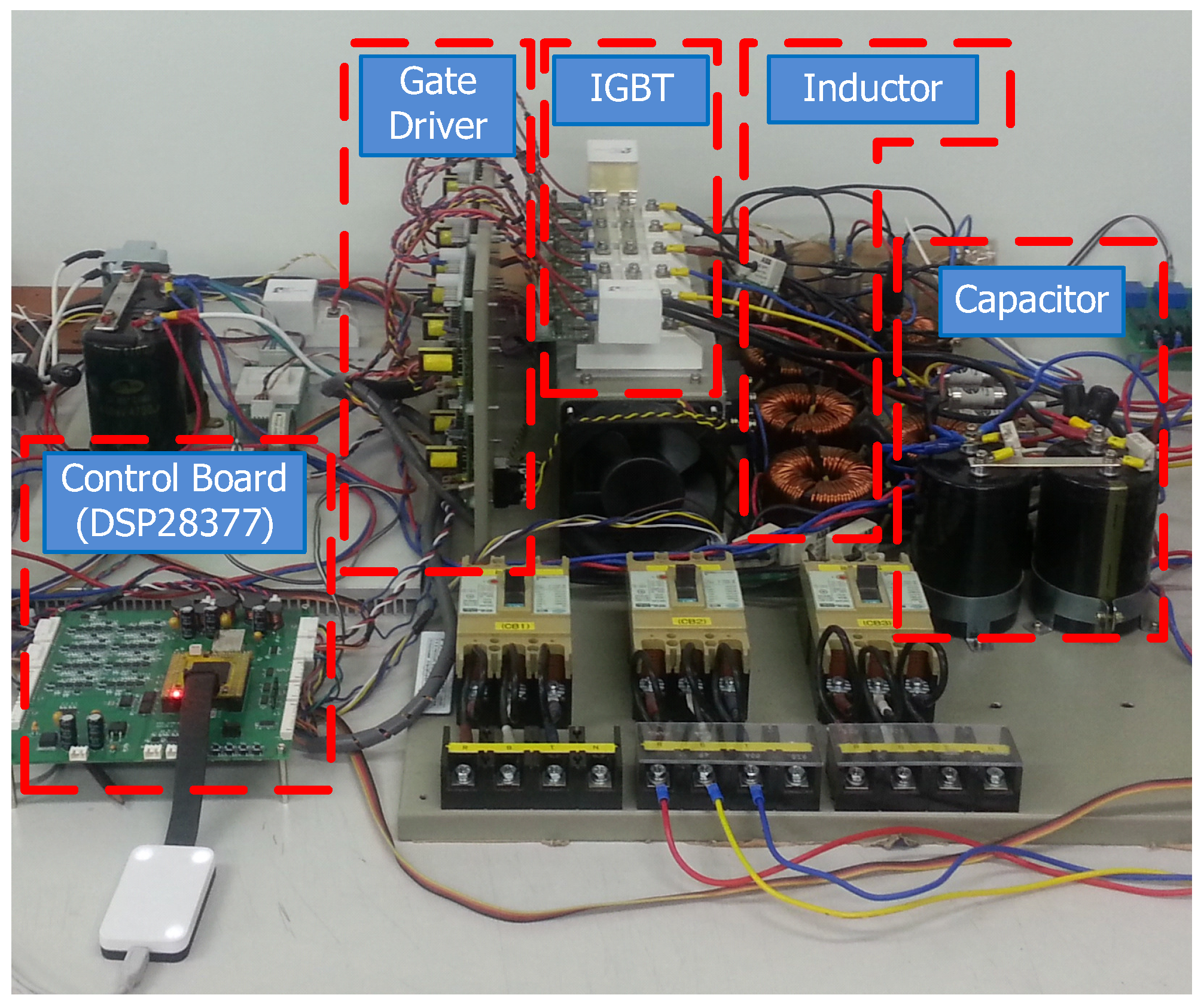
5. Experimental Results

Figure 3 visualizes the experimental setup comprised of the prototype 3 kW three-phase inverter, inductor, output capacitor, and digital signal processor (DSP; Texas Instrument (TI) DSP28377, Dallas, TX, USA) board. The passive component (e.g., inductance and capacitance) values were given as $R=0.038\Omega$, $L=1$ mH, and C = 80 $\mathsf{\mu }$F. The DC-Link level was set to $V_{dc}=90$ V with the bi-directional power supply. The synchronization for control and pulse-width modulation (PWM) periods was done to $0.1$ ms of internal interrupt service routine. An additional laptop PC using MATLAB/Simulink (2022a) was used to observe and collect the real-time system responses, such as current and voltage, under the controller area network environment.

The control algorithms were realized using the nominal parameter values $R_0=0.8$ R, $L_0=1.3$ L, and $C_0=0.9$ C for taking into account the parameter variations in this experimental study. The design parameter tuning result was given as follows: (observer) $k_{obs}=20$, $l_{a_c}=628$, (DOB) $l_v=942$, (self-tuner) ${\gamma }_{st}=20$, ${\rho }_{st}=10/{\gamma }_{st}$, and (active damping) $k_v=5\times {10}^{-3}$ with the cut-off frequency ${\omega }_{vc}=12.56$ rad/s ($f_{vc}={\omega }_{vc}/2\pi =2$ Hz).

The conventional PZC technique comprised of proportional–integral control and feed-forward compensators was chosen for comparison and given by the following specifications [10]:

• (Outer-loop)

  $$\begin{array}{c}\hfill {\mathbf{i}}_{ref}=-b_{d,v}{\mathbf{v}}_c+L_0{\omega }_{vc}{\tilde{\mathbf{v}}}_c+b_{d,v}{\omega }_{vc}{\int }_0^T{\tilde{\mathbf{v}}}_{c}d\tau -C_0{\omega }_r\mathbf{J}{\mathbf{v}}_c\end{array}$$
• (Inner-loop)

  $$\begin{array}{c}\hfill \mathbf{u}=L_0{\omega }_{cc}\tilde{\mathbf{i}}+R_0{\omega }_{cc}{\int }_0^t\tilde{\mathbf{i}}d\tau -L_0{\omega }_r\mathbf{J}\mathbf{i},\tilde{\mathbf{i}}={\mathbf{i}}_{ref}-\mathbf{i},\forall t\ge 0,\end{array}$$

The specifications also included with the additional inclusion of active damping term $-b_{d,v}{\mathbf{v}}_c$ for a better performance and tuned parameters $b_{d,v}=0.5$ and ${\omega }_{cc}=1885$ rad/s ($f_{cc}={\omega }_{cc}/2\pi =300$ Hz); this control also tries to assign the desired cut-off frequency ${\omega }_{vc}$ to the closed-loop system, which is identical to the control objective of proposed controller.

The next sections clarify the practical advantages of the proposed PD-type controller through the comparison study with the PZC controller in the output voltage tracking and regulation tasks under the linear (resistive and resistive–inductive) and nonlinear (rectifier) load variations.

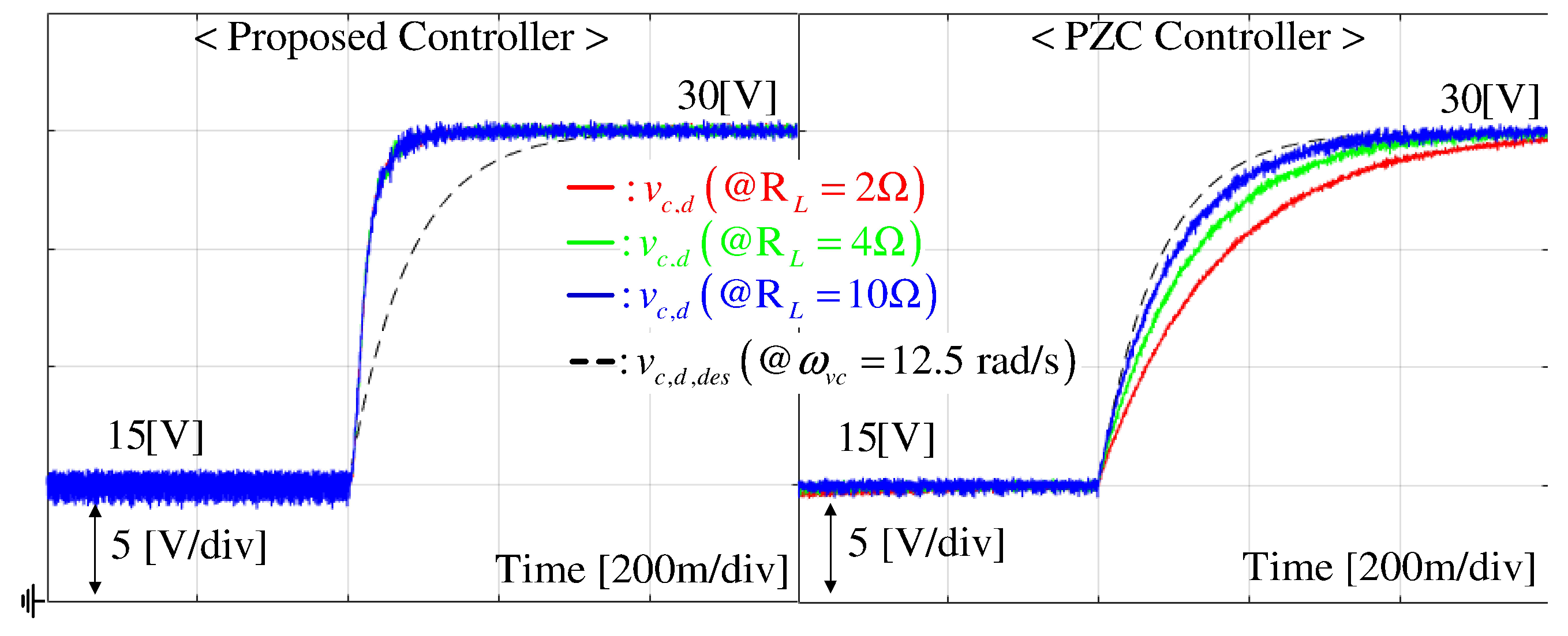
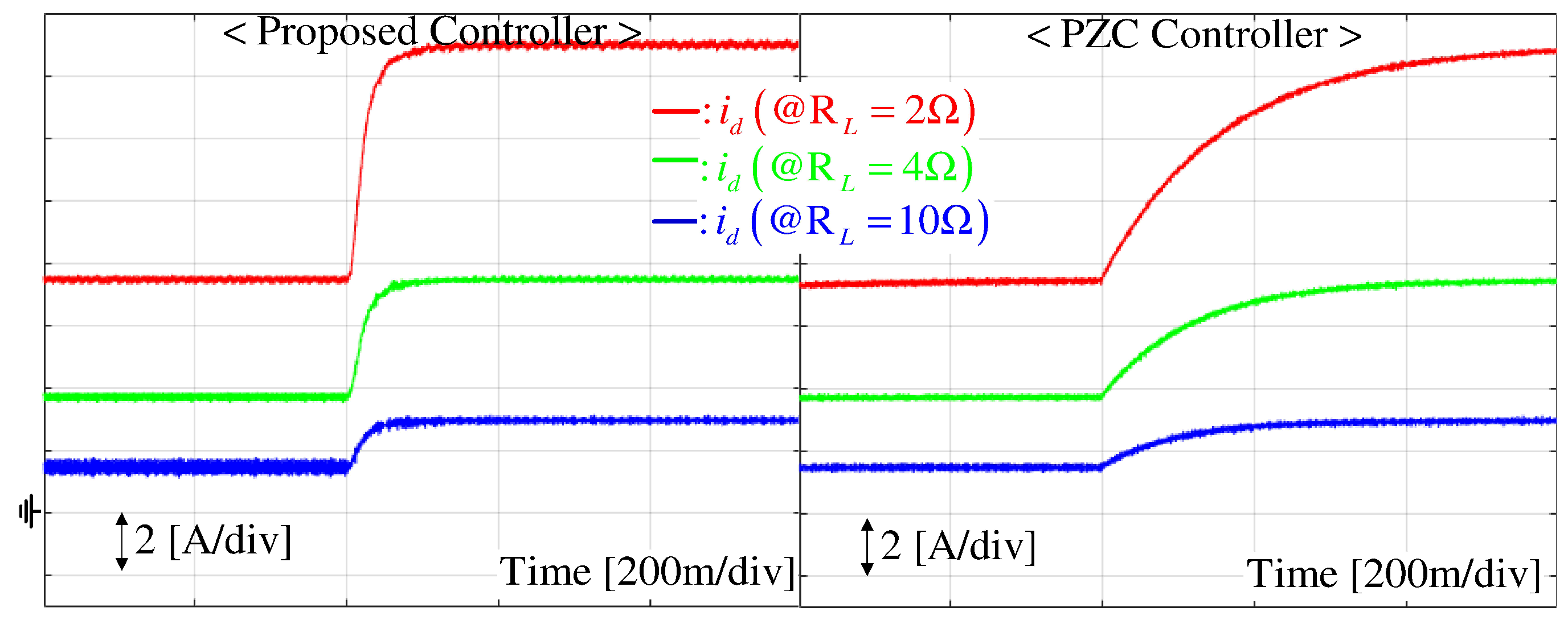
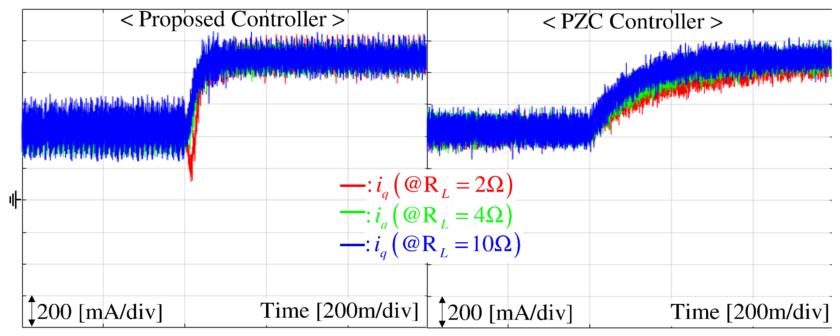
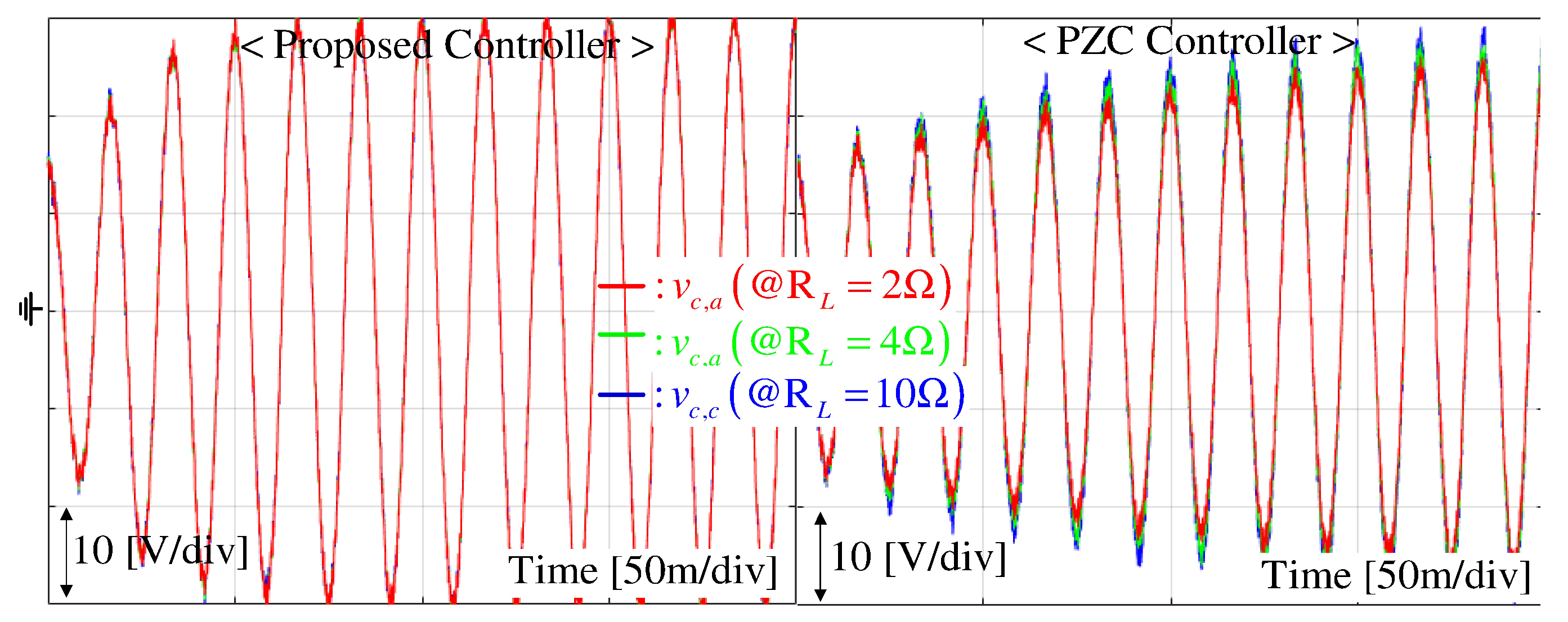
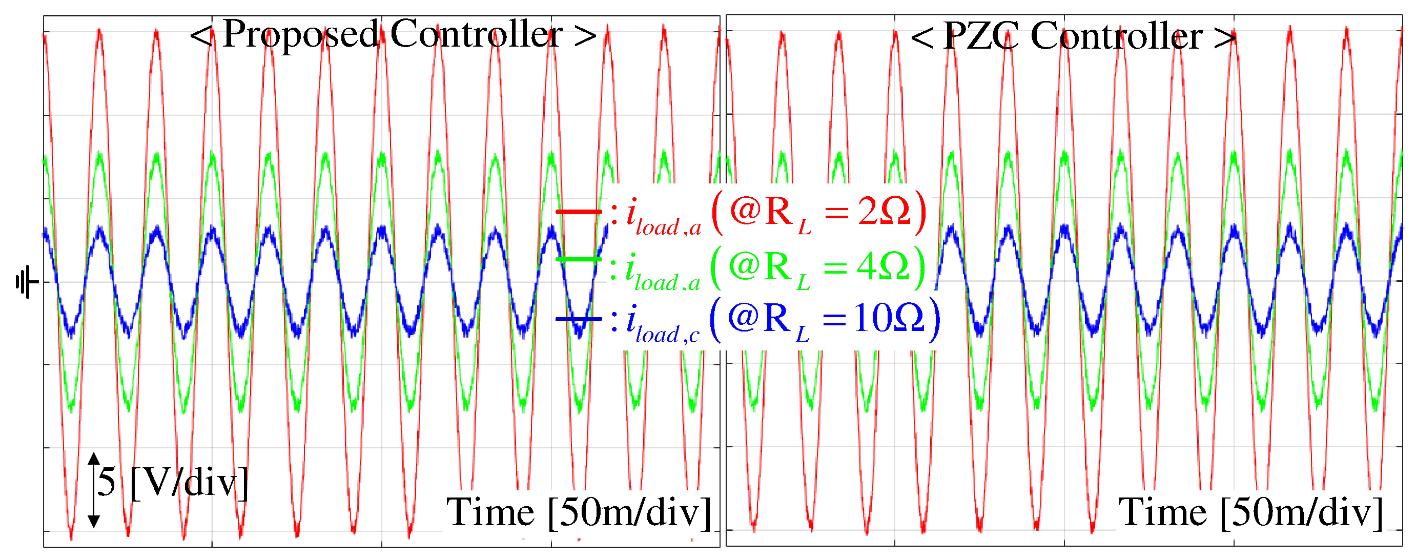
5.1. Performance Comparison for Linear Load Variation

5.1.1. Tracking Task

This section observes the tracking performance variations under the use of three resistive loads $R_L=2$, 4, $10\Omega$. The output voltage reference was suddenly increased from its initial value $r=15$ V to $r=30$ V. Figure 4 shows that there were no tracking performance variations under the proposed control, but they were present under the PZC control, in the absence of current feedback for the proposed control system. Moreover, the proposed self-tuner effectively improved the closed-loop performance in the transient periods by increasing and restoring the feedback gain (e.g., feedback-loop adaptation). This beneficial point comes from the observer, online self-tuner, active damping, and DOBs embedding in the proposed controller. The resultant a-phase voltage responses are depicted in Figure 5 with the consistent closed-loop performance with the proposed controller in the presence of operating condition changes. Figure 6 and Figure 7 show the d-q current responses to be driven more rapidly by the proposed controller than the PZC controller. The load current waveform for each controller is presented in Figure 8, resulting in the total harmonic distortion (THD) calculation result of $1.1\%$ (approximately the same with both controllers), which is acceptable for the actual applications. Figure 9 presents the observer error behaviors in this task with the successful state estimation results by rendering the estimation error to be convergent to zero by the proposed observer. The DOB and self-tuner responses are shown in Figure 10 and Figure 11.

5.1.2. Tracking Task under Resistive–Inductive Load

This section demonstrates the tracking performance variations for three resistive–inductive load pairs of ($R_L=2\Omega$, $L_L=1$ H), ($R_L=4\Omega$, $L_L=1$ H), and ($R_L=10\Omega$, $L_L=1$ H) under the same settings as in Section 5.1.1. Comparing the output voltage responses in Figure 4, Figure 12 indicates the consistent output voltage responses by the proposed controller for resistive and resistive–inductive load operations, unlike the conventional PZC controller. The corresponding a-phase voltage responses are presented in Figure 13 with considerable rapidity and consistency, compared with the PZC controller.

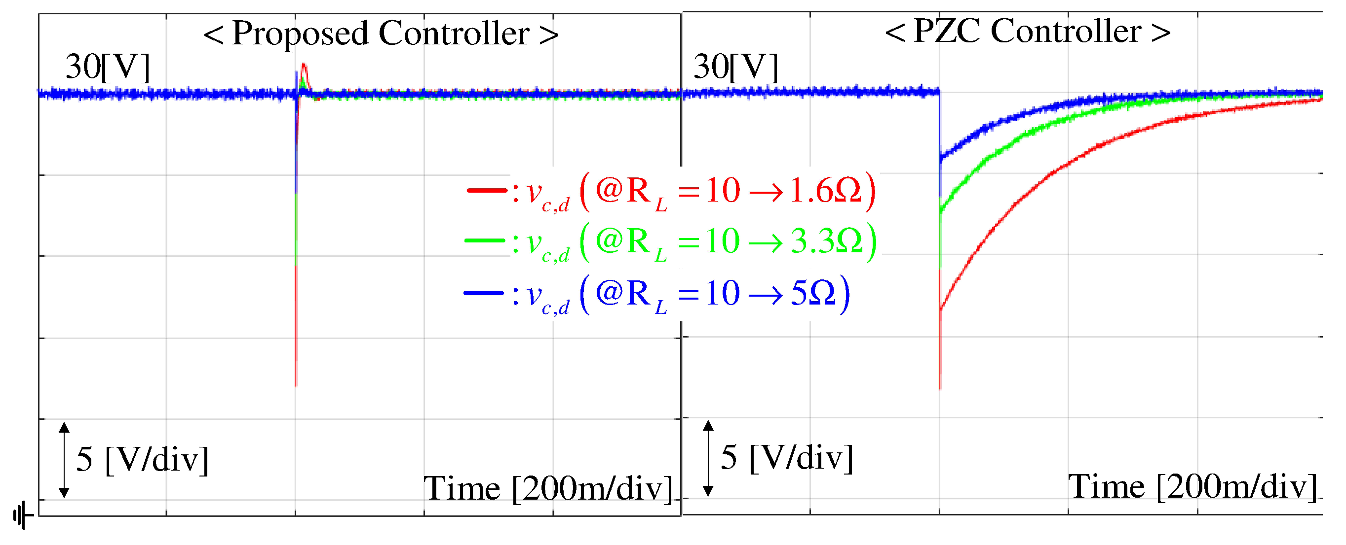
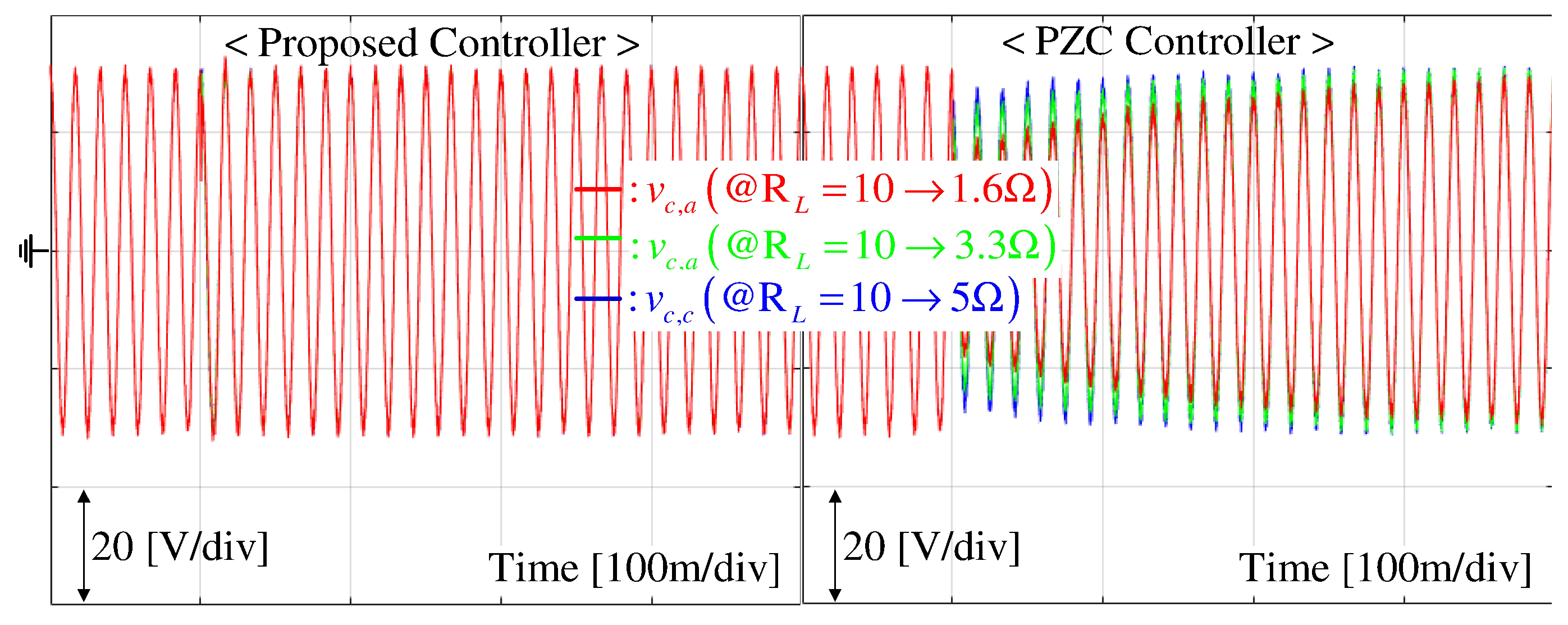
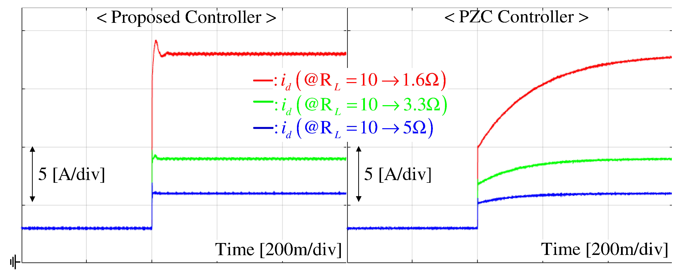
5.1.3. Regulation Task under Resistive Load

This section demonstrates the output voltage regulation performance improvement at the fixed 30 V operation mode with three sudden resistive load change scenarios from the initial resisitve load $R_L=10\Omega$ to $1.6\Omega$, $3.3\Omega$, and $5\Omega$. Figure 14 depicts the regulation performances from the proposed and PZC controllers by showing the d-axis voltage responses. There were significant performance improvements rather than the tracking task under the three load variation scenarios with the considerable reduction of transient periods by the proposed controller. This improvement was also presented in a-phase voltage responses shown in Figure 15. Figure 16 and Figure 17 depict the d-q current whose rapid behaviors result in this output voltage’s regulation performance improvement.

5.2. Performance Comparison for Nonlinear Load Variation

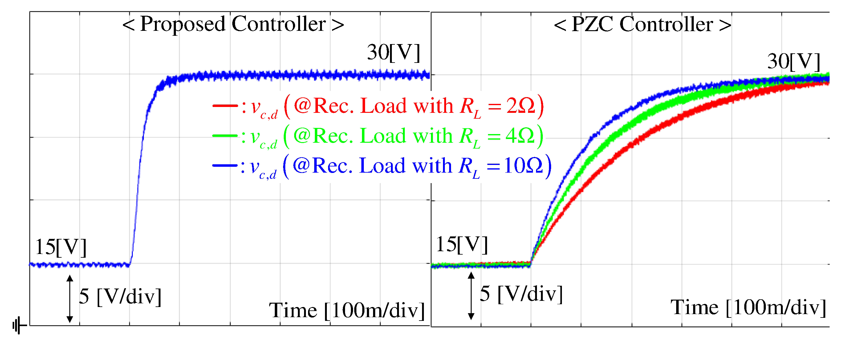
5.2.1. Tracking Task

This section uses the nonlinear loads comprised of the three-phase diode rectifier and single resistor to evaluate the output voltage tracking performance improvement. This experiment was conducted three times for three single resistors of 2, 4, and $10\Omega$. The same output voltage reference for the resistive load case was used. Figure 18 shows similar result as the resistive load case, except for the voltage ripple magnification from the three-phase diode rectifier switching actions. There were no tracking performance variations under the proposed control, but they were present under the classical control, in the absence of current feedback for the proposed control system.

5.2.2. Regulation Task

This section verifies the output voltage regulation performance improvement under the nonlinear load where the resistor value attached in the three-phase diode rectifier was abruptly changed from $10\Omega$ to $1.6$, $3.3$, and $5\Omega$. The output voltage reference was fixed to 30 V. Figure 19 also shows the similar result as the resistive load case, except for the voltage ripple magnification. The proposed controller provided a considerable better regulation performance with the reduction of undershoot magnitude and transient periods.

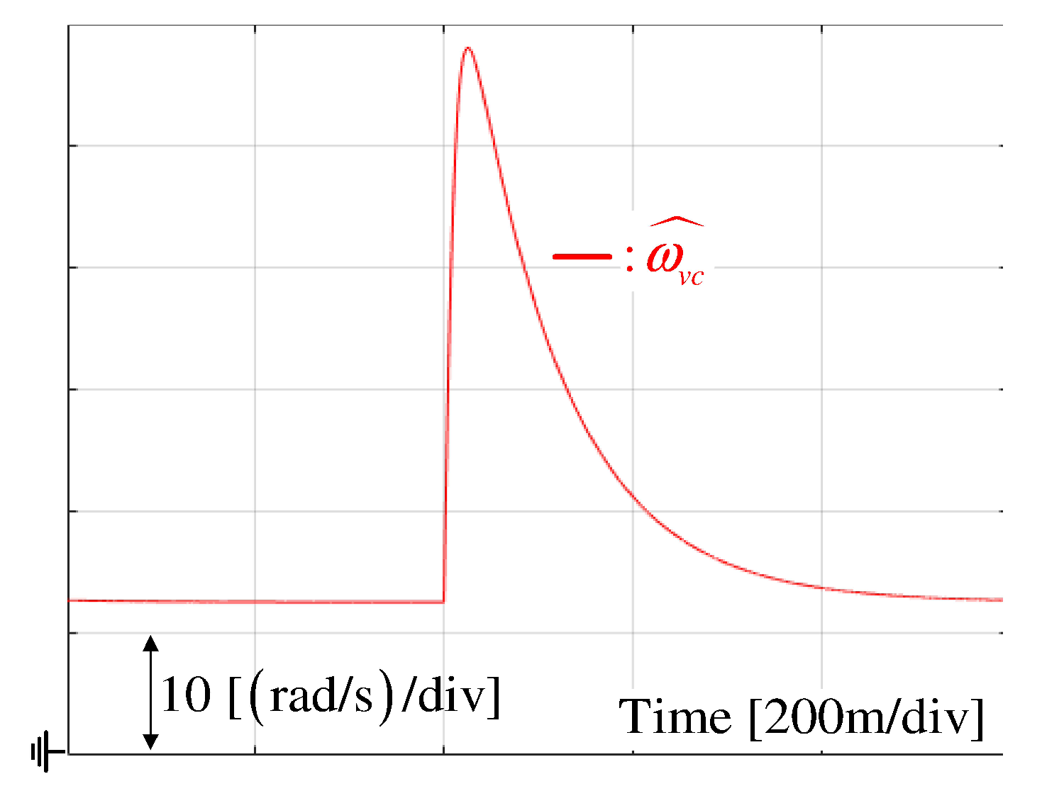
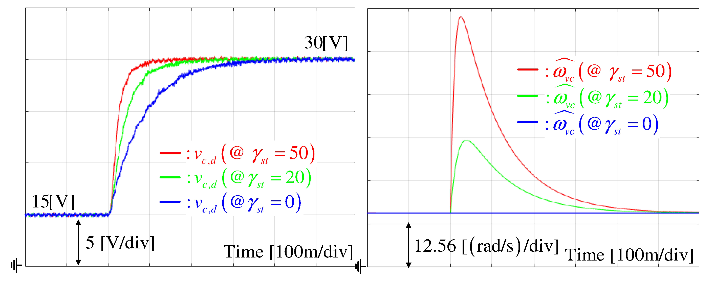
5.3. Tracking Task: Self-Tuner Effect

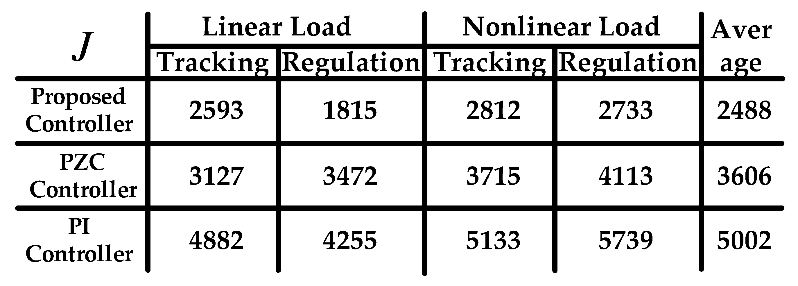
This section presents the merit of variable cut-off frequency from self-tuner under the tracking task with the resistive load $R_L=2\Omega$. The self-tuner design parameter ${\gamma }_{st}$ was increased to 0, 20, and 50 with the step reference from 15 V to 30 V. As intended, Figure 20 shows that the increased cut-off frequency excitation level resulted in the improved tracking performance without any over- or undershoots due to the performance recovery property proved in Theorem 1.

5.4. Summary

This section concludes the experimental studies in Section 5.1 and Section 5.2 by showing the quantitative comparison results obtained from the metric function $J:=\sqrt{{\int }_0^{\infty }{\parallel {\mathbf{v}}_{c,des}-{\mathbf{v}}_c\parallel }^{2}dt}$. This comparison additionally included the case of a conventional multi-loop PI controller tuned for the base bandwidth ${\omega }_{v_c}$. Figure 21 shows the table summarizing the performance comparison results indicating an improvement of $31\%$ at least by the proposed technique.

6. Conclusions

The proposed output voltage regulator was designed without the current feedback with the consideration of practical constraints, system parameter and load variations. The output voltage derivative observer was proposed to estimate the actual state without dependence on system parameters, which removes the need for current feedback. The improved closed-loop robustness was secured by the combination of active damping and specific forms of PD gains, leading to the closed-loop system order reduction to 1. Moreover, the beneficial closed-loop properties, named performance recovery and offset-free, were guaranteed by the closed-loop analysis. The various experimental data verified the practical advantages of the proposed controller. As a future work, the proposed technique will be expanded as a solution to the phase voltage and current synchronization problem for multiple power converters, providing an optimization process to automatically determine the design parameters for the controller, observer, DOB, etc.

References

1. Saeed, M.; Fernández, D.; Guerrero, J.M.; Díaz, I.; Briz, F. Insulation Condition Assessment in Inverter-Fed Motors Using the High-Frequency Common Mode Current: A Case Study. Energies 2024, 17, 470. [Google Scholar] [CrossRef]
2. Patel, M.; Zhou, Z. An Interleaved Battery Charger Circuit for a Switched Capacitor Inverter-Based Standalone Single-Phase Photovoltaic Energy Management System. Energies 2023, 16, 7155. [Google Scholar] [CrossRef]
3. Luo, Z.; Zhang, B.; Li, L.; Tang, L. A Decentralized Control Strategy for Series-Connected Single-Phase Two-Stage Photovoltaic Grid-Connected Inverters. Energies 2023, 16, 7099. [Google Scholar] [CrossRef]
4. Liao, Z.; Peng, T.; Liu, J.; Guo, T. Multi-Adjustment Strategy for Phase Current Reconstruction of Permanent Magnet Synchronous Motors Based on Model Predictive Control. Energies 2023, 16, 5694. [Google Scholar] [CrossRef]
5. Kim, S.K. Performance-recovery proportional-type output-voltage tracking algorithm of three-phase inverter for uninterruptible power supply applications. IET Circuits Devices Syst. 2019, 13, 185–192. [Google Scholar] [CrossRef]
6. Loh, P.C.; Newman, M.J.; Zmood, D.N.; Holmes, D.G. A comparative analysis of multiloop voltage regulation strategies for single and three-Phase UPS systems. IEEE Trans. Power Electron. 2003, 18, 1176–1185. [Google Scholar]
7. Kassakian, J.C.; Schlecht, M.; Verghese, G.C. Principles of Power Electronics; Addison-Wesley: Reading, MA, USA, 1991. [Google Scholar]
8. Matausek, M.R.; Jeftenic, B.I.; Miljkovic, D.M.; Bebic, M.Z. Gain scheduling control of DC motor drive with field weakening. IEEE Trans. Ind. Electron. 1996, 43, 153–162. [Google Scholar] [CrossRef]
9. Sul, S.K. Control of Electric Machine Drive Systems; Wiley: Hoboken, NJ, USA, 2011; Volume 88. [Google Scholar]
10. Kazmierkowski, M.P.; Krishnan, R.; Blaabjerg, F. Control in Power Electronics—Selected Problems; Academic Press: Cambridge, MA, USA, 2002. [Google Scholar]
11. Bustos, R.; Gadsden, S.; Biglarbegian, M.; AlShabi, M.; Mahmud, S. Battery State of Health Estimation Using the Sliding Interacting Multiple Model Strategy. Energies 2024, 17, 536. [Google Scholar] [CrossRef]
12. Xin, C.; Li, Y.X.; Ahn, C.K. Adaptive Neural Asymptotic Tracking of Uncertain Non-Strict Feedback Systems With Full-State Constraints via Command Filtered Technique. IEEE Trans. Neural Netw. Learn. Syst. 2023, 34, 8102–8107. [Google Scholar] [CrossRef]
13. Liu, D.; Zhao, H. Affine Projection Sign Subband Adaptive Filter Algorithm With Unbiased Estimation Under System Identification. IEEE Trans. Circuits Syst. II Express Briefs 2023, 70, 1209–1213. [Google Scholar] [CrossRef]
14. Kawabata, T.; Miyashita, T.; Yamamoto, Y. Deadbeat control of three phase PWM inverter. IEEE Trans. Power Electron. 1990, 5, 21–28. [Google Scholar] [CrossRef]
15. Ito, Y.; Kawauchi, S. Microprocessor-based robust digital control for UPS with three-phase PWM inverter. IEEE Trans. Power Electron. 1995, 10, 196–204. [Google Scholar] [CrossRef]
16. Cho, J.S.; Lee, S.Y.; Mok, H.S.; Choe, G.H. Modified deadbeat digital controller for UPS with 3-phase PWM inverter. In Proceedings of the Industry Applications Conference, Thirty-Fourth IAS Annual Meeting, Phoenix, AZ, USA, 3–7 October 1999. [Google Scholar]
17. Willmann, G.; Coutinho, D.F.; Pereira, L.F.A.; Libano, F.B. Multiple-loop H control design for uninterruptible power supplies. IEEE Trans. Ind. Electron. 2007, 54, 1591–1602. [Google Scholar] [CrossRef]
18. Lee, T.; Tzeng, K.; Chong, M. Robust controller design for a single-phase UPS inverter using μ-synthesis. IEE Proc. Electr. Power Appl. 2004, 151, 334–340. [Google Scholar] [CrossRef]
19. Pichan, M.; Rastegar, H. Sliding-Mode Control of Four-Leg Inverter With Fixed Switching Frequency for Uninterruptible Power Supply Applications. IEEE Trans. Ind. Electron. 2017, 64, 6805–6814. [Google Scholar] [CrossRef]
20. Vargas, R.; Cortes, P.; Ammann, U.; Rodriguez, J.; Pontt, J. Predictive control of a three-phase neutral-point-clamped inverter. IEEE Trans. Ind. Electron. 2007, 54, 2697–2705. [Google Scholar] [CrossRef]
21. Cortes, P.; Rodriguez, J.; Vazquez, S.; Franquelo, L.G. Predictive control of a three-phase UPS inverter using two steps prediction horizon. In Proceedings of the 2010 IEEE International Conference on Industrial Technology (ICIT), Via del Mar, Chile, 14–17 March 2010. [Google Scholar]
22. Cortes, P.; Ortiz, G.; Yuz, J.I.; Rodriguez, J.; Vazquez, S.; Franquelo, L.G. Model Predictive Control of an Inverter With Output LC Filter for UPS Applications. IEEE Trans. Ind. Electron. 2009, 56, 1875–1883. [Google Scholar] [CrossRef]
23. Bemporad, A.; Borrelli, F.; Morari, M. Model predictive control based on linear programming; The explicit solution. IEEE Trans. Autom. Control 2002, 47, 1974–1985. [Google Scholar] [CrossRef]
24. Borrelli, F. Constrained Optimal Control of Linear and Hybrid Systems; Springer: New York, NY, USA, 2003. [Google Scholar]
25. Kim, S.K.; Park, C.; Yoon, T.W.; Lee, Y. Disturbance-observer-based model predictive control for output voltage regulation of three-phase inverter for uninterruptible-powersupply applications. Eur. J. Control 2015, 23, 71–83. [Google Scholar] [CrossRef]
26. Lim, J.; Park, C.; Han, J.; Lee, Y. Robust tracking control of a three-phase DC-AC inverter for UPS applications. IEEE Trans. Ind. Electron. 2014, 61, 4142–4151. [Google Scholar] [CrossRef]
27. Danayiyen, Y.; Lee, K.; Choi, M.; Lee, Y. Model Predictive Control of Uninterruptible Power Supply with Robust Disturbance Observer. Energies 2019, 12, 2871. [Google Scholar] [CrossRef]
28. Nam, N.; Choi, M.; Lee, Y. Model Predictive Control of a Grid-Connected Inverter with LCL Filter using Robust Disturbance Observer. In Proceedings of the IFAC Workshop on Control of Smart Grid and Renewable Energy Systems CSGRES 2019, Jeju, Republic of Korea, 10–12 June 2019. [Google Scholar]
29. Danayiyen, Y.; Altaş, I.; Lee, Y. Robust Discrete Time Disturbance Observer with Finite Control Set Model Predictive Control in UPS System. In Proceedings of the IFAC Workshop on Control of Smart Grid and Renewable Energy Systems CSGRES 2019, Jeju, Republic of Korea, 10–12 June 2019. [Google Scholar]
30. Khalil, H.K. Nonlinear Systems, 3rd ed.; Prentice Hall: Hoboken, NJ, USA, 2002. [Google Scholar]
Figure 1. The UPS system topology.
Energies 17 01738 g001
Figure 2. Proposed control system structure.
Energies 17 01738 g002
Figure 3. Experimental setup.
Energies 17 01738 g003
Figure 4. d-axis output voltage tracking performance variation comparison for three resistive loads R L = 2 , 4, 10 Ω .
Energies 17 01738 g004
Figure 5. a-phase output voltage ( V c , a ) tracking performance variation comparison for three resistive loads R L = 2 , 4, 10 Ω .
Energies 17 01738 g005
Figure 6. d-axis current response comparison under tracking task for three resistive loads R L = 2 , 4, 10 Ω .
Energies 17 01738 g006
Figure 7. q-axis current response comparison under tracking task for three resistive loads R L = 2 , 4, 10 Ω .
Energies 17 01738 g007
Figure 8. a-phase load current response comparison under tracking task for three resistive loads R L = 2 , 4, 10 Ω .
Energies 17 01738 g008
Figure 9. Observer error responses under tracking task for three resistive loads R L = 2 , 4, 10 Ω .
Energies 17 01738 g009
Figure 10. DOB responses under tracking task for three resistive loads R L = 2 , 4, 10 Ω .
Energies 17 01738 g010
Figure 11. Self-tuner response under tracking task for resistive load R L = 10 Ω .
Energies 17 01738 g011
Figure 12. d-axis output voltage tracking performance variation comparison for three resistive–inductive load pairs of ( R L = 2 Ω , L L = 1 H), ( R L = 4 Ω , L L = 1 H), and ( R L = 10 Ω , L L = 1 H).
Energies 17 01738 g012
Figure 13. a-phase output voltage tracking performance variation comparison for three resistive–inductive load pairs of ( R L = 2 Ω , L L = 1 H), ( R L = 4 Ω , L L = 1 H), and ( R L = 10 Ω , L L = 1 H).
Energies 17 01738 g013
Figure 14. d-axis output voltage regulation performance comparison under three resistive load change scenarios as R L = 10 1.6 , 3.3 , 5 Ω .
Energies 17 01738 g014
Figure 15. a-phase output voltage regulation performance comparison under three resistive load change scenarios as R L = 10 1.6 , 3.3 , 5 Ω .
Energies 17 01738 g015
Figure 16. d-axis current response comparison under regulation task for three resistive load change scenarios as R L = 10 1.6 , 3.3 , 5 Ω .
Energies 17 01738 g016
Figure 17. q-axis current response comparison under regulation task for three resistive load change scenarios as R L = 10 1.6 , 3.3 , 5 Ω .
Energies 17 01738 g017
Figure 18. d-axis output voltage tracking performance variation comparison for rectifier load with three resistors of R L = 2 , 4, 10 Ω .
Energies 17 01738 g018
Figure 19. d-axis output voltage regulation performance comparison for rectifier load with three resistor value change scenarios as R L = 10 1.6 , 3.3 , and 5 Ω .
Energies 17 01738 g019
Figure 20. d-axis output voltage tracking performance variations and cut-off frequency behaviors as increasing γ s t = 0 , 20, and 50 under resistive load R L = 2 Ω .
Energies 17 01738 g020
Figure 21. Performance comparison results.
Energies 17 01738 g021
Disclaimer/Publisher’s Note: The statements, opinions and data contained in all publications are solely those of the individual author(s) and contributor(s) and not of MDPI and/or the editor(s). MDPI and/or the editor(s) disclaim responsibility for any injury to people or property resulting from any ideas, methods, instructions or products referred to in the content.