Abstract
In the ongoing debate about the feasibility of enforcing a transition to decentralized energy conversion systems, arguments are often presented that lack scientific rigor. Granted, the issue is multi-faceted and fundamentally multi-disciplinary, and possible solutions strongly depend on the selection of location as well as on local climate and demographics. Furthermore, decentralizing the final energy distribution leads to potential socio-economic considerations that involve value judgements. However, the most serious problem is that media have appropriated the topic and are often publishing opinion papers authored by non-specialists and even by representatives of interest groups. The present paper proposes an approach that is innovative on two counts: first, it treats “final energy” as any other commodity and therefore expands the field of investigation to the problems arising from the decentralization of a generic production line or technological chain; second, it argues that a method solidly rooted in Thermodynamics, the Extended Exergy Accounting, may be used to quantify the total amount of primary exergy resources requested by a decentralized strategy (as opposed to a centralized one), so that a comparison can be performed and discussed on a rational, unbiased and scientific basis. This is an introductory paper that reports some theoretical results of the method: realistic applications are perforce excluded because the idea is that the procedure must be drafted in such a way to be applicable to different socio-economic scenarios and locations and to remain valid under a broad range of boundary conditions.
1. Introduction
The centralization/decentralization option is often discussed in the available literature in a strongly asymmetric fashion: when it concerns the conversion of primary to final energy, the merits of either solution are usually evaluated on the basis of the monetary cost of the kWh to the final user, but when it relates to the production of a material good or of an immaterial service a combination of monetary, environmental and socio-economic indices is used instead.
The first and main goal of this paper is to unify the two approaches: final energy is a commodity, just like cars, machinery, tools, services and consumers’ items. Thus, a unified treatment ought to be adopted to compare competing production lines, whatever the commodity they generate. A second important consideration is that if we want to correctly internalize the so-called Externalities (Labor, Capital and Environmental Remediation Costs), a purely monetary approach does not work [1,2]. On the other hand, it is well known that the most popular socio-economic indicators (GDP, Human Development Index, Bio-Capacity Index, Ecological Footprint, Index of Sustainable Economic Welfare, etc.) do not provide sufficiently accurate, balanced, unbiased and objective criteria decision makers can rely on. (In the current context, these two terms are not synonyms: a multi-criteria evaluation paradigm is “biased” when some weighing implicit in the procedure may skew the overall assessment; it is “non objective” when some of the weighing factors may be chosen arbitrarily by the analyst.) Even the “degree of sustainability”, too often cited in the literature, is rather fuzzy and requires arbitrary value judgements [3,4].
The arguments presented in this study suggest to compare possible alternative production structures on the basis of their equivalent primary exergy consumption: readers are referred to [5,6,7] for the definition and properties of the thermodynamic quantity “exergy” and to [8,9] for the Extended Exergy Accounting method and its applications to system analysis.
When addressing the “sustainability” issue, most authors focus on the need to transition to a Purely Renewable Era, in which all final energy uses are covered by primary or secondary renewable sources. In fact, governments in several industrialized countries have tried to rebalance the current situation -still strongly biased towards fossil conversions- by instituting a Mandatory Renewable Energy Target, usually through a system of incentives based on Renewable Energy Certificates, CO2 (more precisely, GHG) avoidance certificates, CO2 tax, etc.: this approach has given renewable energy sources important competitiveness in a field previously dominated by fossil fuels. Since “renewable” means in practice hydraulic, biomass, solar (thermal and photovoltaic) and wind, inherently “local” in their availability, the idea of generating electricity in the same place -or at a short distance from- the location of the source is appealing and has enjoyed a general consensus among specialists, energy companies and most industrial partners (with the possible exception of local landowners that would rather directly cultivate their land instead of paving the fields with PV panels or plastering them with wind turbines). This is, of course, decentralization. What is often neglected in feasibility studies about decentralized energy conversion systems is the fact that there are hidden costs to it: machinery is produced elsewhere, generally using the country energy mix that is surely not completely renewable, transportation costs are heavily dependent on fossil fuels, and a specialized workforce must be brought in from distant locations to assemble, operate and maintain the “renewable” devices. Over the years, state-funded incentives have been adjusted to compensate for these drawbacks (and sometimes for the loss of land use).
Unfortunately, the merits of decentralization are often overestimated by non-specialists who then publish statements that are plainly incorrect both from an engineering and from a scientific point of view (as an example, see [10,11] and some of the comments to his post, or [12]): therefore, Section 2 below contains a list of some of the most commonly cited pros and cons, annotated with a critical remark.
2. Analytical and Critical List of the Acknowledged Advantages and Disadvantages of Decentralized Production Systems
2.1. What Is Decentralization?
In its original significance, “decentralization” denotes a specific form of organizational structure where the top management delegates decision-making responsibilities and daily operations to middle management and lower subordinates, so that top officials can concentrate on making major decisions while dedicating less time to low-level tasks. If properly managed, such a pyramidal scheme has been almost invariably proven to increase the efficiency of the organization [13]. The concept has been later extended to designate a “commodity production structure” (mostly, final energy) distributed over a territory: this is the sense in which we shall use it here. “To decentralize” an industrial manufacture line means to install several smaller production chains distributed over a territory: the rationale being either to place each decentralized unit “near” the main source of supply or “near” to the final users of that commodity. Here, “near” must be intended in a Pareto sense.
2.2. Advantages of Decentralisation (Most of the Points Discussed in This Section Have Been Extracted from [14])
- (a)
- Higher motivation of local workforce
Several industrial Technical Reports testify that decentralization improves the level of job satisfaction and morale, especially amongst newly appointed local managers. If properly coordinated, it promotes a higher feeling of participation, independence, status and group cohesiveness.
- (b)
- Growth and Diversification
Under decentralization, each product division attains sufficient autonomy to exercise its creativity. In this way, the top-level management can encourage productive and efficient competition amongst different divisions. This practice also helps to internally develop managerial skills that ultimately ensure the growth and continuity of an organization.
- (c)
- Quick Decision Making
Decisions are taken and executed by authorized personnel at the local level. This, in turn, results in faster and accurate action taken by managers who are aware of the real, non-filtered, on-site scenario.
- (d)
- Efficient Communication
Local management is perforce organized in fewer hierarchical levels. This streamlines the communication system.
- (e)
- Ease of Expansion
Decentralization can add momentum to the expansion process of a growing business. This might often result in the opening of new business units in different geographical locations. Decentralized production lines react easily to area-specific requirements, such as, for instance, environmental or health regulations.
- (f)
- Better Supervision and Control
Local, lower-level managers can alter production schedules and work assignments with adequate authority, which leads to greater efficiency in supervision. Performance evaluation of each decentralized unit is easy to perform.
2.3. Disadvantages of Decentralization
- (a)
- Difficult To Coordinate
It is important to consider that substantial autonomy is enjoyed by every single division. In the absence of good monitoring protocols, this makes it difficult to coordinate the overall activities.
- (b)
- External Factors
Both local- (region economics, local trade unions, scarcity or abundance of workforce, transportation facilities, local environmental regulations) and large-scale factors (market uncertainties, tariff systems, demographics, central government intervention) can strongly limit the benefits of decentralization.
- (c)
- Narrow Product Lines
Decentralized product lines need to be adequately broad (in terms of type and amount of generated products) so that they can be organized in autonomous units. This is not possible in small factories with narrow product lines.
- (d)
- Lack of Competence
Lower levels in the organization may lack competent managing skills, adding to the difficulty of operation.
- (e)
- Expensive
In a decentralized production line, both white- and blue-collar employees are encouraged to work harder to achieve the local objectives (see points 2.2.a and 2.2.b above). In return, they can demand and obtain higher salaries, which may become unprofitable for the company, especially if one considers the necessarily higher administration expenses in decentralized enterprises.
- (f)
- Inefficient use of resources
When it comes to the recruitment of trained personnel and the availability of physical facilities, every separate department tries to be self-sufficient. This, in turn, may lead to the underutilization of facilities and duplication of functions: additional control is required on the part of the parent branch.
3. A Review of the Scientific Literature
While the decentralization of energy conversion systems is a well-published topic in Engineering Journals (for recent reviews, see [15,16,17]), the optimal dislocation of strategic industrial lines across a country is usually studied by economists and social scientists (for a review, see [18]). This section offers a limited and succinct description of both lines of investigation, the goal being here to underscore the multi-dimensionality of the problem and of its implications and the unavoidable failure to tackle the problem with purely monetary or purely socio-economic approaches. There is a general consensus that decentralized systems have socio-political implications, not all of which are benign [19], that impact the largest users communities-urban systems [20,21]. Henderson [22] argued that sustaining heavy industry locations in—or near—metropolitan areas can be expected to involve enormous explicit and implicit subsidies that, in the end, represent welfare losses. He added that decentralization of production of standardized heavy industry products into smaller and medium-size cities is generally more efficient. Decentralization is linked to sustainable development as well [4,23], though this issue is still somewhat fuzzy and subject to further investigations. International Agencies are also addressing the problem, and the UN-ESCAP has even issued a roadmap for Southern Asia [24].
The literature about decentralization policies often expresses contrasting positions: while favoring decentralization, Fukuizumi [25] argues that the mix of local sources (hydro, solar, wind) combines with that of the local users (single homes, small communities, small factories…) so that the number of energy consumers, equipment, and demand patterns that must be orchestrated is enormous. Thus, while in the centralized model, more power is generated and distributed when demand peaks, in a decentralized system, demand response is used to manage distribution and grid stability. Rather than recurring to incentives, he argues that a high degree of sophisticated automation and analytics is needed to manage heavily fractionated supply-demand networks. Supporting technologies such as predictive artificial intelligence, machine learning, the Internet of Things, and blockchain are critical to analyzing demand and adjusting how much power is drawn from where across the distributed grid, but these applications have not been fully exploited in the power industry [26,27]. Many relatively low-level techniques still need to be brought to an industrial scale and undergo more standardization before new distributed networks can truly settle down. Clarke-Sather [28] stresses the fundamental dilemma of decentralization: “Centralizing production facilities may reduce costs but perhaps not environmental impacts. Decentralizing a supply chain may reduce transportation costs and environmental impacts but increase capital costs”. Lin et al. [29] analyzed the centralization/decentralization cycles in China from 1949 through 2000, concluding that a combination of mismanagement, ill-guided planning and poor resource allocation strategies resulted in unavoidable loops of “decentralization→disorder→centralization→stagnation→decentralization”. Loops were not observed when decentralization was applied to underdeveloped countries, but several independent studies cast severe doubts on its being a good solution for the respective citizens [30,31,32]. Litvack, Ahmad and Bird [33] present evidence from Eastern and Central Europe and suggest that public services can suffer because of decentralization, at least in the short run. In a similar vein, Crook and Sverrisson [34] have, in fact, provided evidence that decentralization in Colombia, West Bengal and Brazil has had little success in improving service delivery. Some authors find that ill-planned and poorly implemented decentralization led to severe ethical, administrative and social problems in countries as different as Nepal and Bangladesh [35,36] and China and Russia [37,38].
4. Materials and Method
The central idea of the method presented here is to use a thermodynamics-based indicator, the Extended Exergy, to compare different configurations of an energy system. Exergy analysis (ExA in the following) is a well-established method [6,39] that gave origin to several system evaluation protocols [40,41,42,43,44]: it results in a rigorous and accurate quantification of the irreversible losses in a system and provides additional valuable information as to the location and the quantitative entity of these losses. Using ExA, system analysts and engineers can evaluate different configurations and select the “least irreversible” one, which, of course, is expected to result in the minimum consumption of resources: several optimization techniques have been developed that adopt exergy as the objective function, and the results have proven to be invariably superior to any other method of analysis. When analyzing real processes though, other issues enter the picture: environmental remediation (or damage avoidance) costs, direct and indirect maintenance costs, land preparation, end-of-life decommissioning, etc. These are cumulatively called “externalities”, simply because 50 years ago, at the time they started being brought into the evaluation, they were considered to be “external” (i.e., independent of) from the pure “production cost”, defined as a function of the mass and energy flows of the technological process being evaluated. More than four decades of applications have finally and convincingly shown that this is not the case and that different configurations bring about different “externalities”: thus, methods were developed to include them in some kind of optimization procedure, and the process came to be known as “the internalization of externalities”. Without exception, such optimization protocols adopt some convention to link the exergy performance, scale and efficiency of a device to the monetary costs originated by its insertion in the system configuration. In other words, they generate either purely monetary [42] or mixed-type indicators, and quite often, a dyadic (cost and exergy efficiency) or triadic (cost, exergy efficiency, technological level) are used to quantify the results [40] and Pareto-optimize the process parameters.
In 1998 [45], a general procedure was proposed that includes all externalities into a purely physical “exergy cost”: the method is called Extended Exergy Accounting (“EEA” hereinafter) and consists in calculating the equivalent primary exergy of capital, labor and environmental remediation costs. The indicator generated by an EEA is called the Exergy Footprint (“ExF”) of the product: it quantifies the amount of primary resources required to produce a material or immaterial commodity starting from material and energy flows available in the environment. Generality comes at a cost: an EEA analysis is time- and location-dependent, in the sense that to perform it, analysts need local econometric data [46] that are depending on the geographic region in which the system is operating and obviously change in time. Several applications [8,47,48,49,50] have demonstrated though that the use of EEA leads to a substantial improvement in the amount of high level information decision makers can avail themselves of.
A detailed description of the EEA paradigm is offered in [9], and here we shall assume that readers are familiar with the technique. In essence, the Extended Exergy (“EE” if it is measured in W, “ee” if in W/unit) is calculated as follows:
- i.
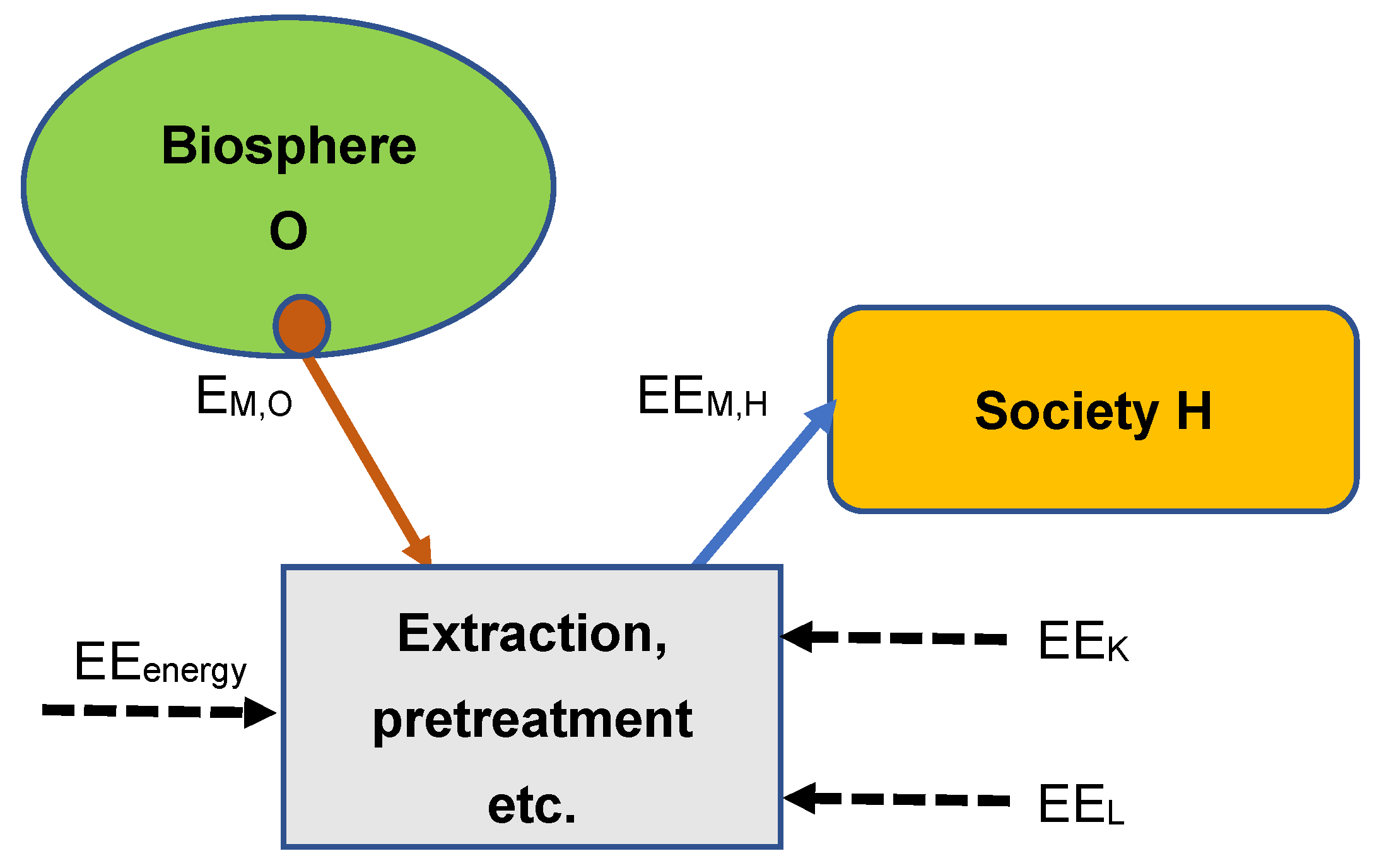
- Material flows are assigned an EE equal to their specific raw exergy (i.e., the exergy per unit mass they possess when in the earth litho-, atmo- or hydrosphere) augmented of all the exergy flows needed for their search, extraction, pre-treatment and transportation to the factory under analysis: this quantity was called Cumulative Exergy Consumption (”CExC”) by Szargut [39]. Since all the above processes involve externalities, proper values are calculated for the EE of capital, labor and environmental costs: the scheme for this calculation is described in detail in [3] and is briefly summarized under points (iii, iv and v) below.
- ii.
- Energy flows directly available in the environment are assigned their equivalent exergy value (in W). If, however, they are “processed” in some way (as when, for example, wind power is converted into electricity), again the EE of the externalities is added (Figure 1).
 Figure 1. The calculation of the EE of a material.
 - iii.
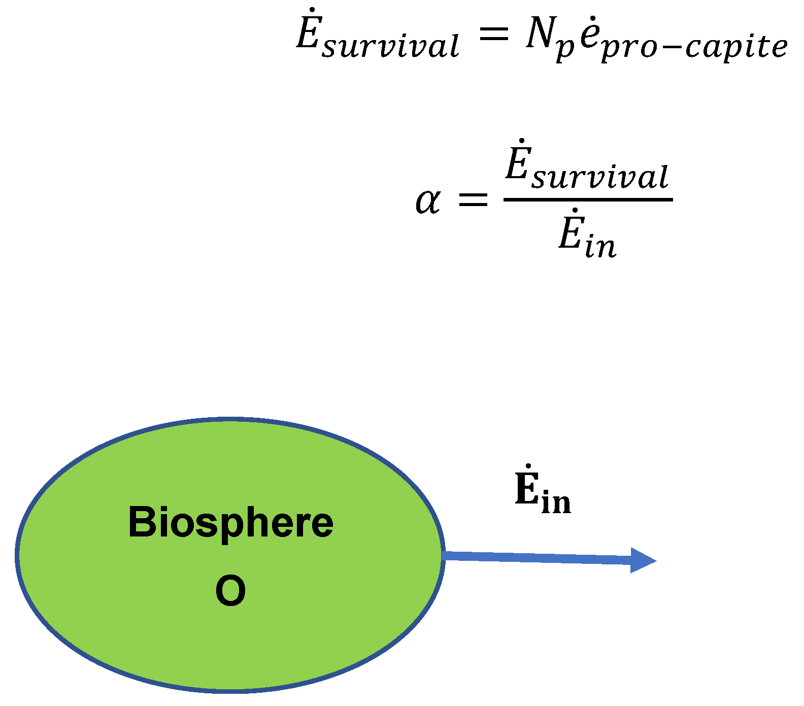
- The specific ee of labor, eeL (J/workhour), is calculated as the total amount of exergy necessary to the sustenance of the population divided by the number of workhours generated in the country: eeL = αEin/(Nw X wh). The econometric coefficient α (Figure 2) is assumed to be known for each country of interest [46]. Thus, the total EE of X workhours is EEL,X = eeL ∗ X (in W).
 Figure 2. Schematic explanation of the calculation of α.
 - iv.
- The EE of Capital, EEK (W), is assumed to be proportional to the Labor EEL, by a second econometric factor β assumed to be known for each country of interest [46]: EEK = βEEL = αβEin. The specific ee of Capital, eeK (J/EUR), is then eeK = αβEin/M2, where M2 (EUR/yr) is a monetary indicator (called “Money plus Quasi-Money”) published monthly/yearly by the Central Banks of all industrialized countries. As a result of the two above postulates, both Labor and Capital become Externalities as well.
- v.
- The environmental externality is calculated by assuming that a proper treatment plant is installed downstream of the system that reduces the physical exergy of the effluents to a value so low that it can be buffered by the biosphere [3,41]. The EEO = (EEM + EEH + EEL + EEK)O of this treatment system is then added to the EEin, and it results in an increase in the resource cost of the product (Figure 3).
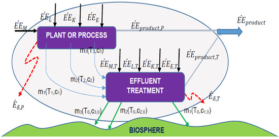 Figure 3. For the calculation of EEO (adapted from [3]). Legenda: .
 - vi.
- Since EE is a “cost” (expressed in W of primary exergy), it obeys a cost conservation rule: the total EE in the input -including all externalities- is always equal to the total EE in the output. Assuming for the moment that the considered process generates N units of a single product, each unit shall be assigned an “extended exergy cost” equal to EEin/N. In the case of multiple products, proper allocation rules must be applied.
- vii.
- Since a correct evaluation of the system must include an exergy flow diagram, each of the N produced units has a unique and unambiguously calculated exergy content EN. Its Exergy Footprint is then a pure number calculated as ExF = EEin/EN: the higher this ratio, the more costly in terms of primary exergy resources the product is.
On the basis of the above, it is possible to compare different system configurations, scales and locations. In this paper, we present a general paradigm to compare two productive structures: one completely centralized and the other with an arbitrary degree of decentralization. Since this preliminary study is aimed at describing the procedure, practical applications are not included, and the examples are evaluated and compared in a rather abstract fashion.
5. The Resource Cost of an Industrial Production Line or Settlement
Consider a generic production system S producing an amount P of a single product, and imagine we wish to compare the two configurations depicted in Figure 4: in the centralized configuration, all material and immaterial inputs Ein enter S in its sole location C and P “units” of the product are released at the same location, while in the decentralized configuration each site Cj generates Pj units of the same product using Ein,j. Notice that we are already using exergy to quantify each single flow (i.e., P is the exergy of the product rather than its mass or numerosity).
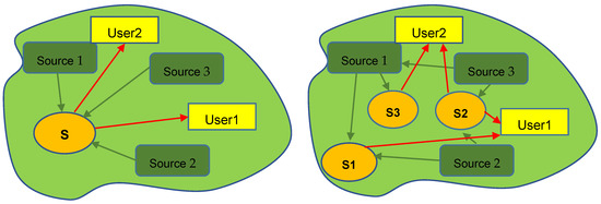
Figure 4.
Centralization vs. decentralization for an industrial plant.
To proceed with a significant comparison, we shall assume that:
- (a)
- The total amount of product is the same in the two cases: ΣPj = P;
- (b)
- The types of raw materials and of energy sources used in both cases are identical;
- (c)
- Due to the plant size (capacity) effect, the efficiency of the decentralized Sj is lower than that of the centralized S by a scaling factor that depends on technological and socio-economic reasons and that we shall assume known for each location: Ein,j/Pj = σjEin/P, the factors σj being higher than unity;
- (d)
- The capital costs are proportional to the size of the plant, but the CAPEX is affected by a cost scaling factor (ψj > 1) as well: ZK,j = ψjPj with ψj > ψ = ZK/P;
- (e)
- A similar reasoning applies to the labor- and maintenance costs (collectively referred to as “OPEX” hereinafter): ZL,j = λjPj with λj > λ = ZL/P. Here, λj > 1;
- (f)
- It is reasonable to assume that the environmental remediation costs scale proportionally to the size of the plant: ZO,j = ωjPj with ωj > ω = ZO/P;
- (g)
- Transportation costs of all inputs are solely proportional to the distance between the source and the plant, and distribution costs to the distance between the plant and the final user: EETR = Σ(τndn) and Σ(EETR,j) = Σ[Σ(τpdq)]j, where the factors τ are specific cost equivalents (W/km) that depend on the transport mode and schedule and on the fuel used (diesel, gasoline, electricity, biofuels…) and must also include their own and separately calculated environmental externality cost EEO,TR,j;
- (h)
- Salaries, interest rate, taxation, environmental regulations, etc., are the same for all locations.
6. A Formal, Resource-Based Cost/Benefit Calculation Procedure
To identify the different merits of each configuration, we simply calculate the ExF of the single product P and compare it with the sum of the ExFj of the decentralized production lines.
For the centralized solution:
EEP = EEM + EEH + EEL + EEK + EEO + EETR
For the fleet of decentralized systems:
Σ(EEPj) = Σ(EEM,j + EEH,j + EEL,j + EEK,j + EEO,j + EETR,j)
Now (point c above)
and therefore (point b) also
Σ(Ein,j) = Σ[(EM,j + EH,j)] = Σ[σjEin(Pj/P)] > Ein
Σ(EEin,j) > EEin
The sum of the EE of the externalities can be expressed (points iii, iv and v above) as
Σ[EEL,j + EEK,j + EEO,j] = eeKΣ[ZL,j + ZK,j + ZO,j] = eeKΣ[λjPj + ψjPj + ωjPj)] > (EEL + EEK + EEO)
To simplify the notation, we can conclude that the sum of the primary resource equivalent of the material, energy, labor, capital and environmental terms in the “budget” of the decentralized system is higher than the corresponding value for the centralized one by a “decentralization cost factor” that is, in turn, a (non-linear) function of the scaling factors σj, φj, λj, ψj and ωj:
Σ[EEL,j + EEK,j + EEO,j] = δ ⟨σj,φj,λj,ψj,ωj⟩(EEL + EEK + EEO)
Thus, a decentralization strategy is convenient only if
Σ(EETR,j)/EETR,j) < δ⟨σj,λj,ψj,ωj⟩
This result is not as trivial as it may seem: in fact, transportation costs include both the CAPEX and OPEX of electrical distribution, road- or rail transportation, etc., and especially for the latter modes, their EEK and EEO are usually the largest contributions to the final cost of the delivered commodity.
7. Discussion
The result obtained in the last section is general, but it paves the way for physically useful calculations. The problem, of course, is to properly and accurately quantify the factor δ: this section offers some practical suggestions on how to proceed. Let us examine the individual parameters on which δ depends.
- (a)
- The efficiency scaling factors σj
For each type of technical process, correlations are available to derive the efficiency penalty that affects plants of smaller capacity. These correlations are often available in the form of tables [51] or nomograms [52] and are constantly updated.
- (b)
- The CAPEX scaling factors ψj
In a completely similar way, reliable correlations are available for estimating at a preliminary process design stage, i.e., prior to the detailed design of the installation, the monetary penalty involved in the “scaling down” of a process.
- (c)
- The OPEX scaling factors λj
Two plants that operate under the same technology have a labor intensity inversely and nonlinearly proportional to their respective capacities: over the years, the industrial practice has resulted in the concoction of reliable algorithms that allow for accurate quantification of this effect. The same applies to maintenance costs.
- (d)
- The exhaust treatment scaling factors ωj
The monetary cost of effluent treatment systems is relatively higher for smaller plants (their CAPEX and OPEX grow inversely to their size, according to points b and c above). Concurrently though, according to the stipulations of points (v) of Section 4 and (c,f) of Section 5, the mass flow rate of the effluent decreases, partially compensating for the increase in the capital and labor costs. Again, numerical calculations are available in the scientific literature [53] so that the ωj can be calculated with sufficient accuracy.
- (e)
- The transportation costs τj
These costs depend on two sets of parameters: the first is purely logistic and includes the source-to-site and site-to-user distances, the mode in which the material and immaterial flows are delivered (road, rail, ship or wire) and the type of connections (status of each connection and geographical/topological details). For all of the above, reliable data exist to calculate the cost in EUR/(ton/km) or EUR/(kWhkm). Since the exergy content of all streams is known, all of these costs can be easily converted into their EE equivalents. The second set of parameters relates to the environmental costs associated with each transportation mode: GHG of rail, road and ship transport are available on the web [54,55], and they can be converted to EE by a “virtual treatment plant” or more simply calculated in terms of the CO2 tax applicable to each mode. Again, the procedure implies the calculation of the monetary costs first and then its conversion to the EE by means of the eeK (point iv, Section 4).
8. Illustrative Examples of Application
In view of the above considerations, two hypothetical benchmark cases are “solved” here.
8.1. Three Smaller Coal-Fed Thermoelectric Plants Substitute for a Single Large One
The values for the coefficients have been calculated, as shown in Table 1. The central 1000 MWel plant S and the three alternatives S1, S2 and S3 are shown in Figure 5 (exergy flow in MW), and the distances (in km) between raw material and energy sources R1, R2 and plant and plant-to-user U1, U2 and U3 are known (Table A1 in Appendix A). The specific extended exergy of capital has been estimated as eeK = 1700 kWh/EUR. Distances are extracted from a Google map; the values for the factors σ, ψ, λ, ω and τ have been adapted from the available literature; installation costs, interest rates, inflation and cost escalation factors are averages of EU values in recent years. The process efficiency of the centralized plant is the state-of-the-art value for RDF-fueled powerplants. The Cumulative Exergy Consumption factor cexc is adapted from [39], and the electrical transmission losses have been adapted from [56]. The emissions per kWh are adapted from [57].

Table 1.
Exergy Footprint of the centralized vs. decentralized configurations, Case A. (ExF in kWhprimary/kWhel).
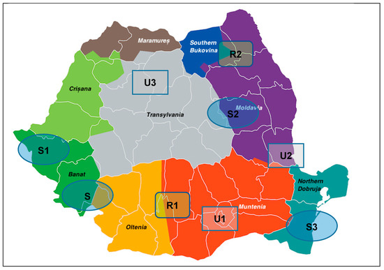
Figure 5.
The examined hypothetical configurations.
Several cases have been evaluated, and the results presented in Table 1 here refer to the following specifications:
Case A: S1, 250 MW; S2, 350 MW; S3, 400 MW. Load allocations proportional to the installed plant capacity.
Case B: Same installed power as above, but the delivered energy is allocated proportionally to the plant-user distance. S1 does not feed U2, which is too distant (see Table A2).
Case C: Same as Case B, but S1, S2 and S3 are more efficient and costlier (see Table A3).
The above results can be now critically summarized:
- In the case of a single, 1000 MW powerplant, the Exergy Footprint ExF of the electrical energy received by the users is 3.42 kWh/kWh (Table 1). This means that for each final kWh, 3.42 kWh of primary resource (coal) have been consumed (and cannot be replaced, since we are dealing with a fossil source);
- The decentralization scheme of Case A (Table 1) is not convenient since the ExF of all users is higher than that of the centralized solution. This effect depends on the scale factors for the CAPEX and OPEX of smaller plants (that increase their respective EEK), on their lower efficiency (that increases the mass of coal used to generate a single kWh) and on their relatively costlier exhaust treatments (higher EEO);
- Optimizing the capacity allocation as in Case B helps (Table 2) but does not solve the problem: the ExF of the decentralized system is still higher than that of the centralized one. Possible optimal sets of solutions may exist and can be sought after by performing an optimization w.r.t. the source-to-plant and plant-to-user distances;
Table 2. Exergy Footprint of the centralized case with the three examined decentralized configurations.
- A convenient solution is that of adopting a better technology for the smaller plants, i.e., raising their efficiency as in Case C (Table 2), because the decrease in environmental costs (lower mass flowrate of coal) more than compensates for the increased CAPEX.
8.2. Three Smaller RDF Incineration Plants Substitute a for Single Large One
Assume now that the plant in S is a 50 MWel RDF incineration process that feeds a steam turbine plant. The values for the coefficients have been calculated, as shown in Table A4 in Appendix A. The central plant S and the three alternatives S1 (25MW), S2 (15MW) and S3 (10MW) are located in the same positions, as in the cases examined in Section 8.1, but now the km between raw material and energy sources R1 and R2 are calculated as road distances extracted from the Google map, while the plant-to-user U1, U2 and U3 are the same as in Section 8.1. Most of the other data are the same, but the installation costs are taken from [58]. The process efficiency of the plants is the state-of-the-art value for RDF-fueled incinerators. The Cumulative Exergy Consumption factor cexc is taken equal to 1 because the RDF is considered as an input “from the environment”, and the transportation costs (by truck) are based on the scheme provided in [55]. The emissions per kWh are adapted from [54].
As shown in Table 3, decentralization leads to higher consumption of primary resources. There are two causes for this: first, the CAPEX is relatively higher for plants of smaller capacity, and second, the total distance of road transportation is almost triple in the decentralized case, and the smaller tonnage of each single branch does not fully compensate for the increased GHG emissions due to the selected road mode. In fact, this example, as preliminary and only approximately accurate as it may be, demonstrates the substantial influence of the road transportation cost. In spite of the quasi-optimized capacity allocation, the GHG emissions from the Diesel-powered trucks overpenalize the decentralized solution, which would have the merit of reducing the source-to-plant and the plant-to-user ton∗km values. The example also suggests that RDF incineration is not always at an advantage w.r.t. a fossil-fueled plant, mostly because of the scale effects on the CAPEX.
Table 3.
Exergy Footprint of the centralized vs. decentralized configurations for RDF-fueled plants. (ExF in kWhprimary/kWhel).
9. Conclusions
Human societies do not survive on monetary capital but on primary resources: once this indisputable fact is accepted, it is clear that the goal of technological development ought to be that of improving the primary-to-final energy conversion chain (irrespective whether the former are fossil or renewable). The Exergy Footprint ExF, an indicator based on the Extended Exergy Accounting method, has proven to be a proper quantifier for this task. In this paper, a general paradigm is proposed to assess the convenience of decentralizing industrial systems. It is shown that the major challenge for a decentralized structure is to reduce both the source-to-plant and plant-to-user transportation costs. In industrialized countries though, while it is possible to build plants of a reasonably large capacity in the immediate proximity of the source, it is almost impossible to devise a decentralized configuration that minimizes the sum of the distances from the commodity-producing plant to the users. The primary-to-final network is strongly interconnected and has several hierarchically organized levels (in the sense that the products at level “i” become the “fuel” at level “i + 1”, where “i” is closer to the source), and thus, the existence of a single and rigorous indicator is beneficial in all cases in which a multi-level, multi-product optimization is considered: when an analyst deals with a complex non-linear system characterized by literally thousands of design- and configuration parameters, the advantage of having a single objective function is apparent. As with any other method, the EEA proposed here to calculate the ExF has its drawbacks: it requires an extremely disaggregated database, not always available and often difficult to retrieve; its results depend on location (in the examples of Section 8, the same analysis applied to a neighboring country would provide entirely different results). Finally, its results depend on the two econometric coefficients α and β, both to be calculated from country statistics and varying in time: thus, a multi-year scenario is necessarily based on extrapolations of their values.
Notwithstanding these problems, the results obtained via stationary applications of the method have been extremely promising and encourage further studies of the method and its applications.
Funding
This research obtained no external funding.
Institutional Review Board Statement
Not applicable.
Informed Consent Statement
Not applicable.
Data Availability Statement
Data is contained within the article.
Conflicts of Interest
The author declares no conflict of interest.
Nomenclature
| Symbol and Units | Meaning | Greek Symbols | |
| c EUR/ton | Specific cost of coal | α | Econometric coefficient |
| CExC (W), cexc | Cumulative exergy consumption | β | Econometric coefficient |
| d km | Distance | δ | EE evaluation factor |
| E (W) | Exergy flow | ε | 2nd Law efficiency |
| EE (W), ee (W/unit) | Extended Exergy | λ | OPEX scaling factor |
| ExF (W/W) | Exergy Footprint | ψ | CAPEX scaling factor |
| fsz | Szargut exergy factor | σ | Efficiency scaling factor |
| GHG | Greenhouse gas | τ | Transportation scaling |
| i (EUR/(EURyear) | Yearly Interest rate | ω | Effluent treatment scaling |
| LHV (kWh/kg) | Lower Heating Value | Suffixes | |
| M2 | Money + Quasi-money | Coal, RDF | Indicated the used fuel |
| NW | Number of Workers | d | Exergy destruction |
| P | Product | F | Fuel |
| PF (h/yr) | Plant factor | H | Energy |
| R | Capital recovery rate | in | input |
| S (MW) | Plant Capacity | L | Labor |
| t | Tons of material | M | Material |
| TIC (EUR) | Installation cost | O | Environmental |
| wh | Number of workhours | TR | Transportation |
| Z | Cost rate | ||
Appendix A
Table A1.
Data for the hypothetical comparison (see Figure 2).
Table A1.
Data for the hypothetical comparison (see Figure 2).
| σ1 | 1.1 | ψ1 | 1.15 | λ1 | 1.15 | ω1 | 1.2 | τ1 | 0.25 |
| σ2 | 1.05 | ψ2 | 1.1 | λ2 | 1.1 | ω2 | 1.15 | τ2 | 0.35 |
| σ3 | 1.03 | ψ3 | 1.05 | λ3 | 1.1 | ω3 | 1.1 | τ3 | 0.4 |
| dR1-S | 200 | dR2-S | 663 | dS-U1 | 300 | dS-U2 | 550 | dS-U3 | 350 |
| dR1-S1 | 424 | dR2-S1 | 607 | dS1-U1 | 500 | dS1-U2 | 650 | dS1-U3 | 300 |
| dR1-S2 | 413 | dR2-S2 | 150 | dS2-U1 | 250 | dS2-U2 | 150 | dS2-U3 | 325 |
| dR1-S3 | 354 | dR2-S3 | 527 | dS3-U1 | 200 | dS3-U2 | 200 | dS3-U3 | 650 |
| ΣdS-U | 1200 | ΣdS1-U | 1450 | ΣdS2-U | 725 | ΣdS3-U | 1050 | PF | 0.628 |
| S | 1000 | S1 | 250 | S2 | 350 | S3 | 400 | eeK | 1.7 |
| TICS | 2.1 × 10⁹ | R(i,30) | 0.06 | εS | 0.39 | kgCO2/kWh | 0.75 | cexc | 1.25 |
| ZF,S | 1.145 | ZK,S | 4 | ZL,S | 0.07 | ZO,S | 4.58 | ed,tr | 0.00008 |
| Eel,S | 174.40 | Ein,S | 447.19 | EEin,S | 558.99 | EEin,tot,S | 577.1 | ccoal | 20 |
| Eδ,S | 5.54 | EU,S | 168.86 | EEU,S | 577.1 | eeel,S | 3.42 |
Table A2.
Modified data for the comparison, case B.
Table A2.
Modified data for the comparison, case B.
| ES1-U1 | 8.37 | ES1-U2 | 0.00 | ES1-U3 | 34.04 |
| ES2-U1 | 25.64 | ES2-U2 | 25.65 | ES2-U3 | 8.49 |
| ES3-U1 | 30.89 | ES3-U2 | 30.89 | ES3-U3 | 6.61 |
Table A3.
Modified data for the comparison, case C.
Table A3.
Modified data for the comparison, case C.
| εS1 | 0.379 | εS2 | 0.382 | εS3 | 0.386 |
Table A4.
Data for the comparison, RDF-fueled plants.
Table A4.
Data for the comparison, RDF-fueled plants.
| σ1 | 1.01 | ψ1 | 1 | λ1 | 1.15 | ω1 | 1.2 | τ1 | 1 |
| σ2 | 1.02 | ψ2 | 1 | λ2 | 1.1 | ω2 | 1.15 | τ2 | 1 |
| σ3 | 1.03 | ψ3 | 1 | λ3 | 1.1 | ω3 | 1.1 | τ3 | 1 |
| dR1-S | 233 | dR2-S | 663 | dS-U1 | 300 | dS-U2 | 550 | dS-U3 | 350 |
| dR1-S1 | 424 | dR2-S1 | 607 | dS1-U1 | 500 | dS1-U2 | 650 | dS1-U3 | 300 |
| dR1-S2 | 413 | dR2-S2 | 150 | dS2-U1 | 250 | dS2-U2 | 150 | dS2-U3 | 325 |
| dR1-S3 | 354 | dR2-S3 | 527 | dS3-U1 | 200 | dS3-U2 | 200 | dS3-U3 | 650 |
| ΣdS-U | 1200 | ΣdS1-U | 1450 | ΣdS2-U | 725 | ΣdS3-U | 1050 | PF | 0.41 |
| EU1 | 19 | EU2 | 16.5 | EU3 | 14.5 | cexc | 1 | eeK | 1.7 |
| S | 50 | S1 | 25 | S2 | 15 | S3 | 10 | fsz,RDF | 1.2 |
| ES1-U1 | 0.57 | ES1-U2 | 0.00 | ES1-U3 | 2.28 | emistr | 0.15 | ed,tr | 0.00008 |
| ES2-U1 | 0.80 | ES2-U2 | 0.57 | ES2-U3 | 0.34 | LHVRDF | 20,000 | CO2 tax | 35 |
| ES3-U1 | 0.57 | ES3-U2 | 0.46 | ES3-U3 | 0.11 | kgCO2/kWh | 0.6 | eeel, S | 3.90 |
| tRDF,R1-S | 60,000 | tRDF,R2-S | 60,000 | tCO2,R1-S | 2097 | tCO2,R2-S | 5967 | zconferral | 15 |
| TICS | 2.95 × 10⁸ | R(i,30) | 0.06 | ZK,S | 0.56 | ZL,S | 0.04 | ZO,S | 0.13 |
| εS | 0.27 | Ein,S | 21.09 | EEin,S | 21.09 | EEin,tot, S | 21.53 | ||
| Eel S | 5.69 | Eδ,S | 0.18 | EU,S | 5.51 | EEU,S | 21.53 |
References
- Ruiz-Villaverde, A. Editor’s Introduction: The Growing Failure of the Neoclassical Paradigm in Economics. Am. J. Econ. Sociol. 2019, 78, 13–34. [Google Scholar] [CrossRef]
- Sylos Labini, F. Science and the Economic Crisis; Springer International Pub.: Cham, Switzerland, 2016; ISBN 978-3-319-29527-5. [Google Scholar]
- Sciubba, E. A Thermodynamic Measure of Sustainability. Front. Sustain. 2021, 2, 739395. [Google Scholar] [CrossRef]
- Wall, G.; Gong, M. Exergy and sustainable development, Part 1: Conditions and concepts. Int. J. Exergy 2001, 1, 128–145. [Google Scholar] [CrossRef]
- Dewulf, J.; van Langenhove, H.; Muys, B.; Bruers, S.; Bakshi, B.R.; Grubb, G.F.; Paulus, D.M.; Sciubba, E. Exergy: Its potential and limitations. Environ. Sci. Technol. 2008, 42, 2221–2232. [Google Scholar] [CrossRef] [PubMed]
- Kotas, T. The Exergy Method of Thermal Plant Analysis, Butterworths; Academic Press: London, UK, 1985. [Google Scholar]
- Moran, M.J.; Sciubba, E. Exergy analysis-principles and practice. JERT 1994, 116, 1994. [Google Scholar] [CrossRef]
- Colombo, E.; Rocco, M.; Sciubba, E. Advances in exergy analysis: A novel assessment of the Extended Exergy Accounting method. Appl. Energy 2013, 113, 1405–1420. [Google Scholar]
- Sciubba, E. Beyond Thermoeconomics? The concept of Extended Exergy Accounting and its application to the analysis and design of Thermal Systems. Exergy Int. J. 2001, 1, 68–84. [Google Scholar] [CrossRef]
- Coote, D. The Benefits of Decentralized Energy; News Corp Australia: Surry Hills, Australia, 2021. [Google Scholar]
- Hagemann, T. Five Reasons to Switch to Decentralised Electricity Generation. The Governance Post, 6 April 2017. [Google Scholar]
- ISGF—India Smart Grid Forum. Characteristics of Smart Grid? How Is It Different from the Existing Grid? Available online: https://indiasmartgrid.org/sgg2.php (accessed on 4 September 2021).
- Siraganyan, K.; Dasun-Perera, A.T.; Scartezzini, J.-L.; Mauree, D. Eco-Sim: A parametric Tool to Evaluate the Environmental and Economic Feasibility of Decentralized Energy Systems. Energies 2019, 12, 776. [Google Scholar] [CrossRef]
- TOPPR Tutorials. Available online: https://www.toppr.com/guides/fundamentals-of-economics-and-management/organising/advantages-and-disadvantages-of-decentralisation/ (accessed on 2 September 2021).
- Alstone, S.; Gershenson, D.; Kammen, D. Decentralized energy systems for clean electricity access. Nat. Clim. Chang. 2015, 5, 305–314. [Google Scholar] [CrossRef]
- Bohn, D. Decentralised energy systems: State of the art and potentials. Int. J. Energy Technol. Policy 2005, 3, 1–11. [Google Scholar] [CrossRef]
- Schütz, T.; Hu, X.-L.; Fuchs, M.; Müller, D. Optimal design of decentralized energy conversion systems for smart microgrids using decomposition methods. Energy 2018, 156, 250–263. [Google Scholar] [CrossRef]
- Sujarwoto, S. Why decentralization works and does not work? A systematic literature review. JSAS 2017, 1, 1–10. [Google Scholar]
- Bolton, S.; Farrell, J. Decentralization, Duplication and Delay. J. Political Econ. 1990, 98, 803–826. [Google Scholar] [CrossRef]
- Adil, A.M.; Ko, Y. Socio-technical evolution of Decentralized Energy Systems: A critical review and implications for urban Planning and Policy. Renew. Sustain. Energy Rev. 2016, 57, 1025–1037. [Google Scholar] [CrossRef]
- Tan, L.-M.; Arbabi, H.; Densley-Tingley, D.; Brockway, S.E.; Mayfield, M. Mapping resource effectiveness across urban systems. Npj Urban Sustain. 2021, 1, 20. [Google Scholar] [CrossRef]
- Henderson, J.V. Locational pattern of heavy industries: Decentralization is more efficient. J. Policy Model. 1988, 10, 569–580. [Google Scholar] [CrossRef]
- Karger, C.R.; Hennings, W. Sustainability evaluation of decentralized electricity generation. Renew. Sustain. Energy Rev. 2009, 13, 583–593. [Google Scholar] [CrossRef]
- UN-ESCAP. Low Carbon Green Growth Roadmap for Asia and the Pacific:Fact Sheet- Decentralized Energy System. Available online: https://www.unescap.org (accessed on 9 September 2021).
- Fukuizumi, Y. 3 Trends That Will Transform the Energy Industry. 2020. Available online: https://spectra.mhi.com/3-trends-that-will-transform-the-energy-industry (accessed on 4 September 2021).
- Egger, G.; Chaltsev, D.; Giusti, A.; Matt, D.T. A deployment-friendly decentralized scheduling approach for cooperative multi-agent systems in production systems. Procedia Manuf. 2020, 52, 127–132. [Google Scholar] [CrossRef]
- Suvarna, M.; YaS, K.S.; Yang, W.; Li, J.; Ng, Y.T.; Wang, X. Cyber-physical production systems for data-driven, decentralized, and secure manufacturing—A perspective. Engineering 2021. Available online: https://www.sciencedirect.com (accessed on 24 July 2021).
- Clarke-Sather, A.R. Decentralized or Centralized Production: Impacts to the Environment, Industry, and the Economy. Ph.D. Thesis, Western Michigan University, Kalamazoo, MI, USA, 2009. [Google Scholar]
- Lin, J.-Y.; Tao, R.; Liu, M.-X. Decentralization and Local Governance in China’s Economic Transition. In Rise of Local Governments in Developing Countries; London School of Economics: London, UK, 2003. [Google Scholar] [CrossRef]
- Agrawal, A.; Ostrom, E. Collective Action, Property Rights, and Decentralization in Resource Use in India and Nepal. Politics Soc. 2001, 29, 485–514. [Google Scholar] [CrossRef]
- Bardhan, P.; Mookherjee, D. Decentralization and Local Governance in Developing Countries: A Comparative Perspective; MIT Press: Cambridge, MA, USA, 2006; Volume 1. [Google Scholar]
- Ribot, J.C. Waiting for Democracy: The Politics of Choice in Natural Resource Decentralization; World Resources Institute: Washington, DC, USA, 2004. [Google Scholar]
- Litvack, J.; Ahmad, J.; Bird, R. Rethinking Decentralization at the World Bank: A Discussion Paper; World Bank Pub: Washington, DC, USA, 2010. [Google Scholar]
- Crook, R.; Sverrisson, A. To What Extent Can Decentralised Forms of Government Enhance the Development of Pro-Poor Policies and Improve Poverty-Alleviation Outcomes? IDS Working Paper 130; Inst. Development Studies: Brighton, UK, 2001. [Google Scholar]
- Bienen, H.; Kapur, D.; Parks, J.; Riedinger, J. Decentralization in Nepal. World Dev. 1990, 18, 61–75. [Google Scholar] [CrossRef]
- Sarker, M.A.; Itohara, Y. Farmers’ perception about the extension services and extension workers: The case of organic agriculture extension program by PROSHIKA. Am. J. Agric. Biol. Sci. 2008, 4, 332–337. [Google Scholar] [CrossRef]
- Blanchard, O.; Shleifer, A. Federalism with and without Political Centralization: China versus Russia; National Bureau of Economic Research: Cambridge, MA, USA, 2000; NBER Paper 7616. [Google Scholar]
- Treisman, D. Decentralization and the Quality of Government, Preliminary Draft Dated November 20, 2000. Available online: https://www.imf.org (accessed on 2 October 2021).
- Szargut, J.; Morris, D.R.; Steward, F.R. Exergy Analysis of Thermal, Chemical, and Metallurgical Processes; Hemisphere Pub.: New York, NY, USA, 1988. [Google Scholar]
- El Sayed, Y.M. The Thermo-Economics of Energy Conversion; Elsevier: Amsterdam, The Netherlands, 2003. [Google Scholar]
- Szargut, J.; Ziębik, A.; Stanek, W. Depletion of the Unrestorable Natural Exergy Resources as a Measure of the Ecological Cost. Energy Convers. Manag. 2002, 43, 1149–1163. [Google Scholar] [CrossRef]
- Tsatsaronis, G. Combination of Exergetic and Economic Analysis in Energy-Conversion Processes. In Proceedings of the European Congress Energy Economics & Management in Industry, Algarve, Portugal, 2–5 April 1984; Pergamon Press: Oxford, UK, 1984; Volume 1, pp. 151–157. [Google Scholar]
- Valero, A.; Lozano, M.A.; Muñoz, M. A general theory of exergy savings-1. On the exergetic cost. Comput.-Aided Eng. Energy Syst. Second Law Anal. Model. 1986, 3, 1–8. [Google Scholar]
- Yantovsky, E.I. Energy and Exergy Currents (An Introduction to Exergonomics); Nova Science Pub.: New York, NY, USA, 1994. [Google Scholar]
- Sciubba, E. A novel exergetic costing method for determining the optimal allocation of scarce resources. In Proceeding Contemporary Problems in Thermal Engineering; Rudnicki, G., Stanek, W., Nowak, A., Eds.; Polytechnica Slaska Publication: Gliwice/Katowice/Zabrze/Rybnik, Poland, 1998; pp. 311–324. [Google Scholar]
- Sciubba, E. A revised calculation of the econometric factors α- and β for the Extended Exergy Accounting method. Ecol. Model. 2011, 222, 1060–1066. [Google Scholar] [CrossRef]
- Biondi, A.; Sciubba, E. Extended Exergy Analysis (EEA) of Italy, 2013–2017, Energies, Extended Exergy Analysis (EEA) of Italy, 2013–2017. Energies 2021, 14, 2767. [Google Scholar] [CrossRef]
- Dai, J.; Chen, B.; Sciubba, E. Ecological accounting for China based on Extended Exergy—A sustainability perspective. Renew. Sustain. Energy Rev. 2014, 37, 334–347. [Google Scholar]
- Estervåg, I. Energy, exergy, and extended-exergy analysis of the Norwegian society. Energy 2003, 30, 649–675. [Google Scholar]
- Seçkin, C.; Sciubba, E.; Bayulken, A.R. An application of the Extended Exergy Accounting method to the Turkish Society, year 2006. Energy 2012, 40, 151–163. [Google Scholar] [CrossRef]
- Ha, G.-H.; Kim, S.H. Cost Scaling Factor according to Power Plant Capacity Change. J. Energy Eng. 2013, 22, 283–286. [Google Scholar] [CrossRef]
- Celikbilek, O. An Experimental and Numerical Approach for Tuning the Cathode for High Performance IT-SOFC. Ph.D. Thesis, Imperial College London, London, UK, 2006. [Google Scholar]
- Hendricks, T.J.; Yee, S.; LeBlanc, S. Cost Scaling of a Real-World Exhaust Waste Heat Recovery Thermoelectric Generator: A Deeper Dive. J. Electron. Mater. 2016, 45, 1751–1761. [Google Scholar] [CrossRef]
- European Environmental Agency. Greenhouse Gas Emissions from Transport in Europe. 2020. Available online: https://www.eea.europa.eu (accessed on 2 October 2021).
- Posada, F.; Chambliss, S.; Blumberg, K. Costs of Emission Reduction Technologies For Heavy-Duty Diesel Vehicles; ICCT paper; World Resources Institute: Washington, DC, USA, 2016. [Google Scholar]
- Pavičić, I.; Holjevac, N.; Ivanković, I.; Brnobić, D. Model for 400 kV Transmission Line Power Loss Assessment Using the PMU Measurements. Energies 2021, 14, 5562. [Google Scholar] [CrossRef]
- ISPRA. GHG Atmospheric Emission Factors in the Electric Sector in European Countries; TR. 317/2020; ISPRA: Roma, Italy, 2020. (In Italian) [Google Scholar]
- Wu, J.S.-Y. Capital Cost Comparison of Waste-to-Energy (WTE) Facilities in China and the U.S. Ph.D. Thesis, Columbia University, New York, NY, USA, 2016. [Google Scholar]


Disclaimer/Publisher’s Note: The statements, opinions and data contained in all publications are solely those of the individual author(s) and contributor(s) and not of MDPI and/or the editor(s). MDPI and/or the editor(s) disclaim responsibility for any injury to people or property resulting from any ideas, methods, instructions or products referred to in the content. |
© 2024 by the author. Licensee MDPI, Basel, Switzerland. This article is an open access article distributed under the terms and conditions of the Creative Commons Attribution (CC BY) license (https://creativecommons.org/licenses/by/4.0/).