Abstract
Medium–long-term photovoltaic (PV) output forecasting is of great significance to power grid planning, power market transactions, power dispatching operations, equipment maintenance and overhaul. However, PV output fluctuates greatly due to weather changes. Furthermore, it is frequently challenging to ensure the accuracy of forecasts for medium–long-term forecasting involving a long time span. In response to the above problems, this paper proposes a medium–long-term forecasting method for PV output based on amplitude-aware permutation entropy component reconstruction and the graph attention network. Firstly, the PV output sequence data are decomposed by ensemble empirical mode decomposition (EEMD), and the decomposed intrinsic mode function (IMF) subsequences are combined and reconstructed according to the amplitude-aware permutation entropy. Secondly, the graph node feature sequence is constructed from the reconstructed subsequences, and the mutual information of the node feature sequence is calculated to obtain the graph node adjacency matrix which is applied to generate a graph sequence. Thirdly, the graph attention network is utilized to forecast the graph sequence and separate the PV output forecasting results. Finally, an actual measurement system is used to experimentally verify the proposed method, and the outcomes indicate that the proposed method, which has certain promotion value, can improve the accuracy of medium–long-term forecasting of PV output.
1. Introduction
Solar energy, as a clean and renewable energy technology, has received widespread attention under the dual pressure of the global energy crisis and environmental pollution. However, the photovoltaic(PV) output, which has obvious volatility and uncertainty, is greatly influenced by natural factors such as sunlight conditions, climate, and seasons. The integration of large-scale PV output may have an impact on the stability of the power grid [1,2,3,4]. Medium–long-term forecasting can be beneficial for power station planning and resource assessment, ensuring the balance of electricity in the power system and improving PV penetration at the macro level [5].
In PV output forecasting, time–frequency decomposition is widely used to handle the volatility of PV power time series due to its ability to reveal the internal structure and local characteristics of the time series. Reference [6] uses the empirical mode decomposition (EMD) signal processing algorithm to decompose the time series into a series of relatively stable component sequences, and then establishes forecasting models for each subsequence. Finally, the forecasting results of each subsequence are stacked to obtain the final forecasting value. Reference [7] introduces the ensemble empirical mode decomposition (EEMD) signal processing algorithm, decomposes historical PV time series into multiple frequencies, and establishes a generalized regression neural network forecasting model to forecast the future output of PV power plants. Reference [8] introduces the Variational Mode Decomposition (VMD) algorithm to avoid mode mixing, boundary effects, and other issues, thereby reducing the non-stationary nature of PV data. Time-frequency decomposition can decompose complex PV power time series into multiple intrinsic mode functions with different frequency characteristics [9,10,11]. The intrinsic mode function can better reveal the intrinsic structure and local characteristics of data, and more accurately capture the dynamic characteristics of PV power changes. In addition, time–frequency decomposition also helps to reduce the complexity of data, improve the generalization ability and forecasting accuracy of the model.
The traditional PV power medium–long-term forecasting method based on time–frequency decomposition usually models each intrinsic mode function obtained from decomposition, forecasts the evolution trend of each intrinsic mode function time series, and then overlays the forecasting results to obtain the final PV power forecasting value. Although each intrinsic mode function is independent in frequency, there may be statistical correlations between them, which can result in similar information entropy [12]. Taking the PV power time series as an example, the decomposed intrinsic mode function may represent rapid power fluctuations caused by cloud cover, or may be related to seasonal changes. Therefore, how to handle the correlation between the modal functions obtained from the decomposition of PV power time series is an important issue.
In deep learning methods, graph neural networks (GNN) are often used to handle multi time series forecasting in various fields [13,14,15]. Reference [16] uses graph convolutional neural networks to capture the topological relationships of power networks, transform them into graphical structures, and transform load forecasting problems into graph node regression tasks, achieving load forecasting. Reference [17] first uses the visibility graph method to transform multiple time series of power loads into undirected graphs, and then trains the GNN with the obtained graph and corresponding adjacency matrix inputs. Finally, real data from high-voltage/medium-voltage substations confirmed that the proposed method outperforms widely used machine learning methods. Reference [18] proposes a traffic flow forecasting model based on a dynamic graph recursive network, which captures hidden spatial dependencies in data through a dynamic graph generator. The generated dynamic graph is trained into special time series data through a dynamic graph recursive neural network, and the excellent forecasting accuracy of the proposed model is verified with a large number of datasets.
The literature indicates that the graph attention network (GAT) in GNN has shown great potential in processing graph structured data [19,20]. GAT allocates adaptive weights to nodes in the graph by introducing attention mechanisms, thereby capturing complex relationships between nodes. Due to its flexibility and generalization ability, it can effectively handle graph structure data from different fields and performs well in various graph related machine learning tasks such as node classification and forecasting, and graph classification [21]. Reference [22] proposes a new dynamic multi granularity spatiotemporal GAT framework for traffic forecasting, which effectively considers the cyclic patterns in traffic data by utilizing the multi granularity spatiotemporal correlations of different time scales and variables. Finally, the effectiveness of the proposed model was verified through simulation. Reference [23] uses GAT to analyze individual speech features to recognize or verify the speaker’s identity, improves the feature fusion strategy in speaker recognition tasks, and enhances recognition performance through a self supervised learning framework. Reference [24] combines GAT with forecast protein contact maps for forecasting whether multi-stage proteins can crystallize, and demonstrate the effectiveness of GAT through simulation experiments.
Although GAT has shown excellent performance in multiple time series forecasting tasks in various fields, it is currently less applied in the field of PV power forecasting. Based on the above background, this paper proposes a medium–long-term PV power forecasting method that combines the time–frequency decomposition algorithm and GAT. By decomposing PV time series using the time–frequency decomposition method and based on amplitude-aware permutation entropy (AAPE), this paper reconstructs the decomposed sequence into a multivariate time series and uses graph attention networks to capture the correlation between various time series, achieving medium–long-term forecasting of PV power. AAPE can be imagined as a special video editor that can split a video into different video tracks. Just like when we watch a video, we can see the picture and hear the sound. AAPE does something similar. It breaks down a complex signal into several simpler parts, each with its own characteristics, and eliminates the parts that have minimal impact. The advantage of this is that we can more easily understand these signals. This article converts the simple parts decomposed by AAPE into nodes, and the GAT is the technology used to more effectively capture complex interactions between nodes. It is like a graph of a social network, which can help us understand the connections between different nodes and predict their subsequent changes.
The method proposed in this paper provides a new feasible approach for medium–long-term forecasting of PV output. The contributions of this paper are as follows:
- (1)
- A PV power feature extraction method based on AAPE is proposed. Through AAPE analysis, the changing characteristics of PV power generation time series are effectively captured, providing a new quantitative description method for PV power generation fluctuation patterns.
- (2)
- A method is creatively designed to convert the reconstructed sequence into node features and adjacency matrix form as the input of GAT. And the relationship between nodes is extracted through the attention mechanism, allowing the model to focus on nodes that are more important to the prediction task.
- (3)
- The proposed algorithm is empirically evaluated in a campus PV-microgrid demonstration system in East China and a public dataset in Australia, respectively. By comparing with existing technologies, the effectiveness and superiority of the proposed method in PV power prediction at different time scales are verified.
2. IMF Component Reconstruction of PV Output Sequences Based on Amplitude Perception Permutation Entropy
2.1. EEMD Decomposition of PV Output Sequences
EEMD automatically separates PV power sequences at different time scales to their corresponding reference scales by adding Gaussian white noise to the original PV output sequence and performing multiple EMD decomposition, effectively suppressing EMD mode aliasing [25] and possessing stronger scale separation ability. The process of EEMD decomposition for is as follows:
Firstly, add Gaussian white noise to , i.e.,
where is the m-th PV power sequence after adding Gaussian white noise.
Then, perform EMD decomposition on to obtain J intrinsic mode function (IMF) components and residual component , i.e.,
Finally, calculate the mean of the IMF and residual components obtained after M rounds of EMD decomposition as shown in Equations (3) and (4), From this, () and are obtained as the nth IMF component and residual component obtained by EEMD decomposition of the original PV power sequence, respectively.
2.2. IMF Component Reconstruction Based on Amplitude Perception Permutation Entropy
The n IMF components and residual components obtained by EEMD decomposition of the PV power series contain local features of the original PV power series at different time scales. However, indiscriminate forecasting and stacking of too many components can not only be computationally cumbersome, but may also lead to error accumulation. Therefore, this paper proposes an IMF component reconstruction method based on amplitude-aware permutation entropy (AAPE). Using AAPE as a measure of sequence complexity, IMF components are classified and reconstructed according to their complexity. This not only reduces time and computational costs, but also provides conditions for using different forecasting algorithms for sequences with different complexities.
Using the theory of phase space reconstruction, the decomposed components of PV output can be reconstructed into vectors as shown in Equation (5)
where and are the embedding dimension and delay time, respectively, , is the total length of the PV power sequence. Arrange the elements in each sequence of in ascending order of size, and denote the th order as . The probability of the occurrence of each order of is as follows:
where represents the number of occurrences of arrangement order ; represents the probability of occurrence of arrangement order .
The permutation entropy (PE) can be calculated from Equation (7)
where represents the calculated value of the PV power sequence component PE. However, PE only considered the order of amplitude in the PV power sequence components, and did not fully extract the amplitude characteristics of the elements in the components. This paper uses the AAPE algorithm to evaluate the complexity of PV power sequence components. Compared to traditional PE algorithms, AAPE considers the deviation between the mean and amplitude of the sequence amplitude in the calculation process, and uses relatively normalized probabilities to replace the counting rules in traditional PE algorithms [26]. The average value (AA) and relative amplitude (RA) of the reconstructed sequence can be represented as follows:
The initial value of is set to 0, and during the process of t in reconstructing vector gradually increases from 1 to , Whenever the order of arrangement is , is calculated once. The formula is as follows:
where is the weight used to adjust the mean amplitude of the component and the deviation between component amplitudes, generally taken as 0.5. The probability of each arrangement order appearing at this time is
Then, the AAPE of the PV power sequence component can be expressed as
where represents the AAPE value of the PV power sequence component. AAPE reflects the complexity of each component, with IMF components with higher AAPE values representing the characteristics of short period components with stronger randomness in PV power sequences, and IMF components with lower AAPE values representing the trend of long period changes with stronger regularity in PV power sequences.
From the perspective of feature extraction, forecasting and modeling components with similar complexity separately have limited effect on improving forecasting accuracy and will greatly increase the workload of model training. To improve the training efficiency of the forecasting model, this paper uses the AAPE difference between adjacent components as the judgment condition to reconstruct the EEMD component. When the AAPE difference between adjacent subsequences is greater than a certain value, it can be considered that there is a significant difference in complexity between components, and they need to be processed separately as subsequences S1~Sz. When the AAPE difference between adjacent components is less than a certain value, it can be considered that the complexity between components is close, and the components contain similar information, which can be merged and recorded as Sz+1.The residual component generally has a large difference from adjacent components and is used as a separate subsequence Sz+2.
3. PV Output Forecasting Modeling Based on the Graph Attention Network
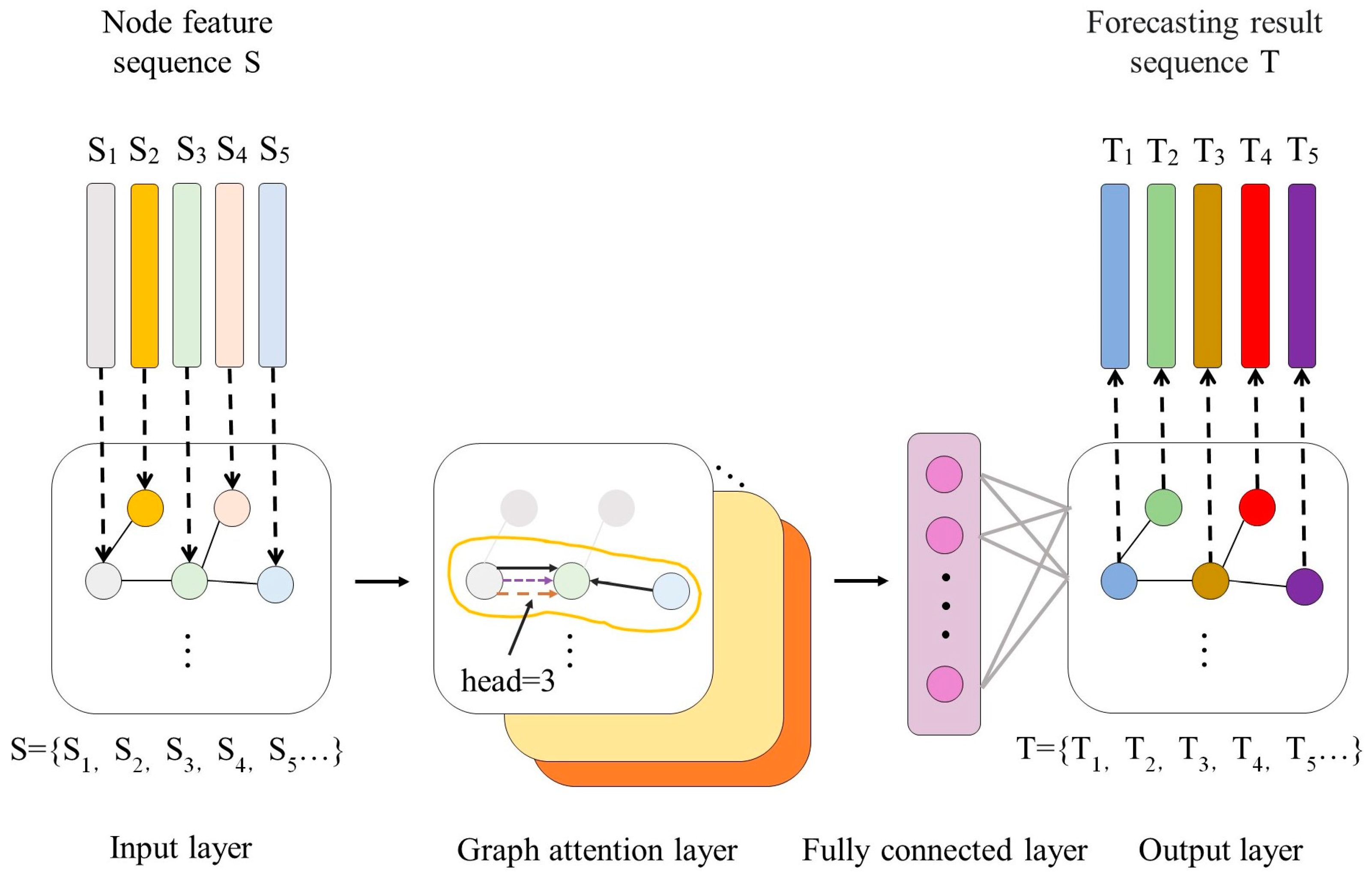
GAT introduces an attention mechanism into graph neural networks based on spatial domains. Unlike graph convolutional networks (GCNs) based on spectral domains, graph attention networks do not require complex calculations using matrices such as Laplacian, and only update node features through the representation of first-order neighboring nodes. The algorithm principle is relatively simple [27,28]. Taking the five subsequences formed after decomposition and reconstruction of the original sequence as an example, the GAT forecasting model constructed in this paper is shown in Figure 1. The model consists of a graph data input layer, a graph attention layer, a fully connected layer, and an output layer.
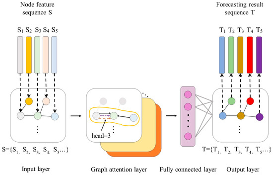
Figure 1.
Structure of GAT.
At the input layer, the node feature sequence and node adjacency matrix obtained from the PV power decomposition and reconstruction sequence together constitute the graph data sequence. Among them, the node feature sequence is composed of the subsequence set S obtained from reconstructing the PV power sequence through the IMF component based on AAPE, where the nodes in each graph data are column elements of the node feature sequence. The edges of each graph data in the graph data sequence are elements of the node adjacency matrix. In this paper, the node adjacency matrix is composed of the mutual information between any two subsequences and in the node feature sequence, as shown in Equations (13) and (14).
where A is the node adjacency matrix; n is the number of nodes; represents the mutual information between and ; is the joint probability of variables and ; and are the edge probability density functions of and respectively.
The core of the GAT neural network is the graph attention layer, which uses an attention mechanism to calculate the hidden representation of each node in the graph, that is, the hidden features of factors in the PV power sequence. Each layer inputs a set of node features and outputs a new set of node features. Firstly, in order to enable the model to obtain sufficient expressive power to transform input features into higher-level features, at least one learnable linear transformation is required to be applied to each node. Therefore, a shared linear transformation parameterized by a weight matrix is used in the attention layer of the graph, and the attention coefficients shown in Equation (15) are calculated for the nodes [29].
where represents the attention coefficient of node j’s features to node I which is the unidirectional relationship between each subsequence of the PV power sequence, and the number attention coefficient calculation head in this paper is 3; and represent node features.
Then, the GAT neural network allows for interaction between each node by injecting the graph structure into the mechanism using attention mechanisms to compute , , where is an adjacent node. In order to make the coefficients easy to compare between different nodes, the softmax function shown in Equation (16) is used to normalize the attention system [30].
Next, the attention mechanism of each layer in the GAT neural network serves as a single-layer feedforward neural network, parameterized by a weight vector and non-linearized using LeakyReLU with a negative slope of 0.2. The specific formula is as follows [31]:
where is the attention mechanism coefficient of node to node ; is the weight vector of the attention mechanism; is the weight matrix; represents transpose operation; represents the splicing operation. Finally, through fully connected layers for feature integration, the sequence forecasting results are output, and the sequence is stacked to obtain the PV output at the time of forecasting.
4. A Combined Forecasting Model Based on the AAPE-GAT Neural Network
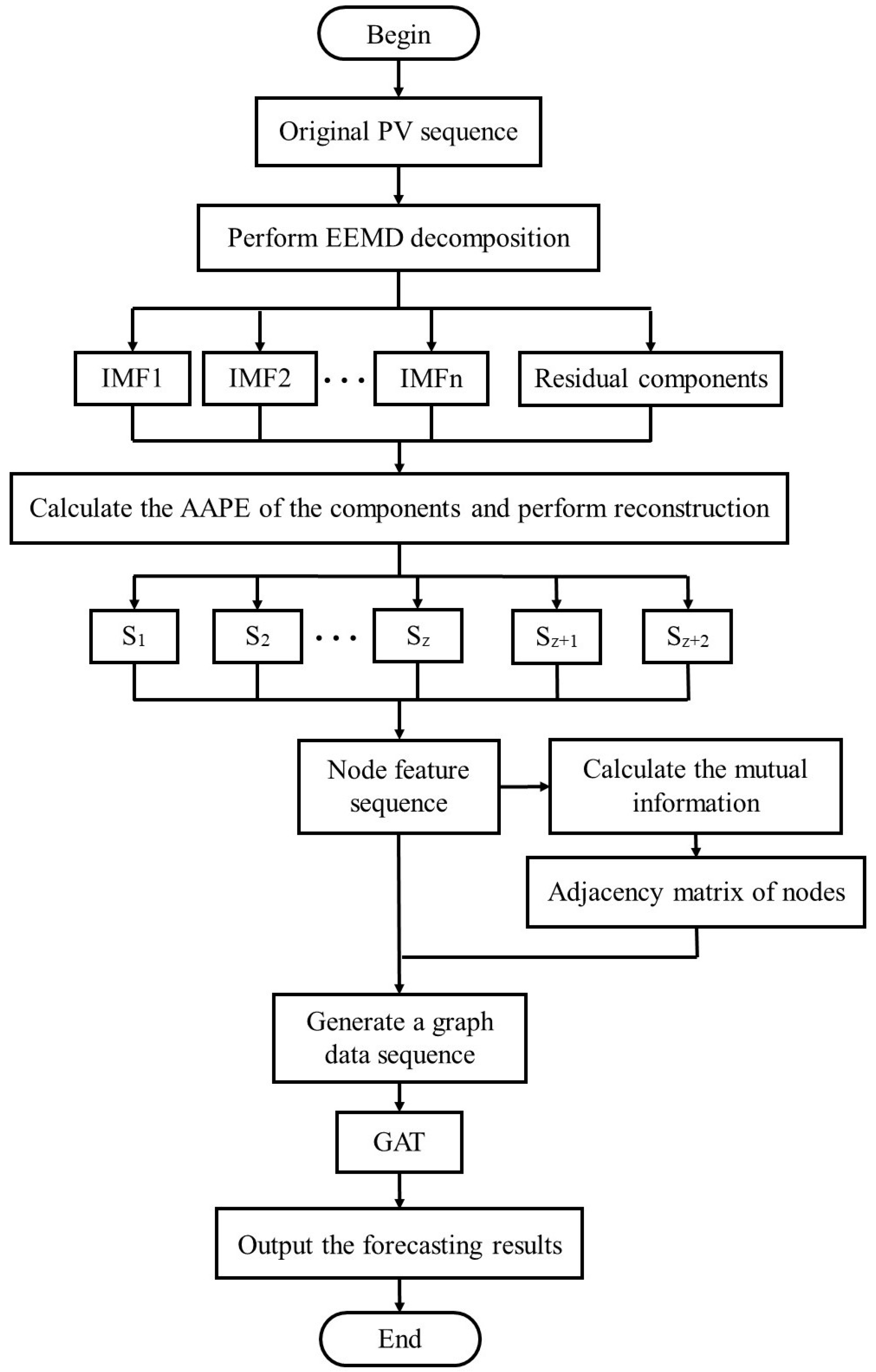
In summary, considering the factors of forecasting accuracy and forecasting time, the proposed AAPE-GAT neural network combination forecasting process in this paper is shown in Figure 2.
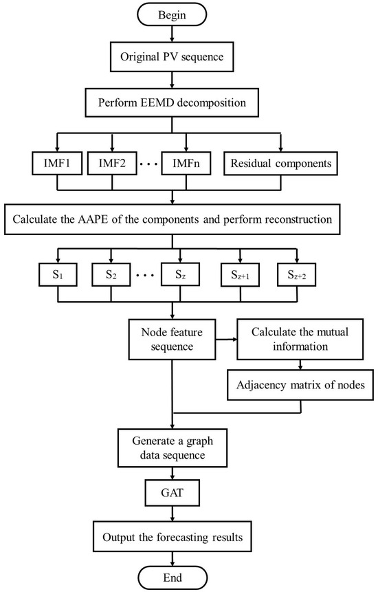
Figure 2.
Forecasting process of AAPE-GAT.
- (1)
- Perform EEMD decomposition on the PV sequence data in the dataset to obtain IMF and residual components for different frequency components.
- (2)
- Calculate the AAPE of the components and perform reconstruction to obtain the node feature sequence.
- (3)
- Calculate the mutual information of node feature sequences to obtain the adjacency matrix of nodes, and generate a graph data sequence together with the node feature sequence.
- (4)
- Input the graph data sequence into the GAT neural network, and finally output the forecasting results.
5. Example Analysis
5.1. Datasets and Preprocessing
The simulation and verification of this paper uses the PV output power data collected from the PV output system of Hangzhou Dianzi University(HDU) from January 2022 to January 2024 as the dataset. The installed capacity of the PV system is 120 kWp, and the sampling period is from 8:00 to 17:00 every day, with a sampling interval of 60 min. Therefore, the number of sampling points per day is 10. The original data consists of 820 days, corresponding to 8200 sampling points. To obtain statistical results, this paper constructs a time series of raw data for training and forecasting, using 730 days from January 2022 to December 2023 as the training set, using the last 90 days as the forecasting set. The forecast time span is 15 days.
To test the generalizability and robustness of the proposed forecasting model from different geographical locations, we also apply our model to the dataset from the Desert Knowledge Australia Solar Centre (DKASC), Alice Springs which contains a range of solar technologies operating at Desert Knowledge Precinct in Central Australia. The sampling period is from 8:00 to 17:00 every day, with a sampling interval of 60 min. We use 730 days from January 2021 to December 2022 as the training set, using the last 90 days as the forecasting set and the forecast time span is 15 days.
5.2. EEMD Decomposition of PV Output Sequence
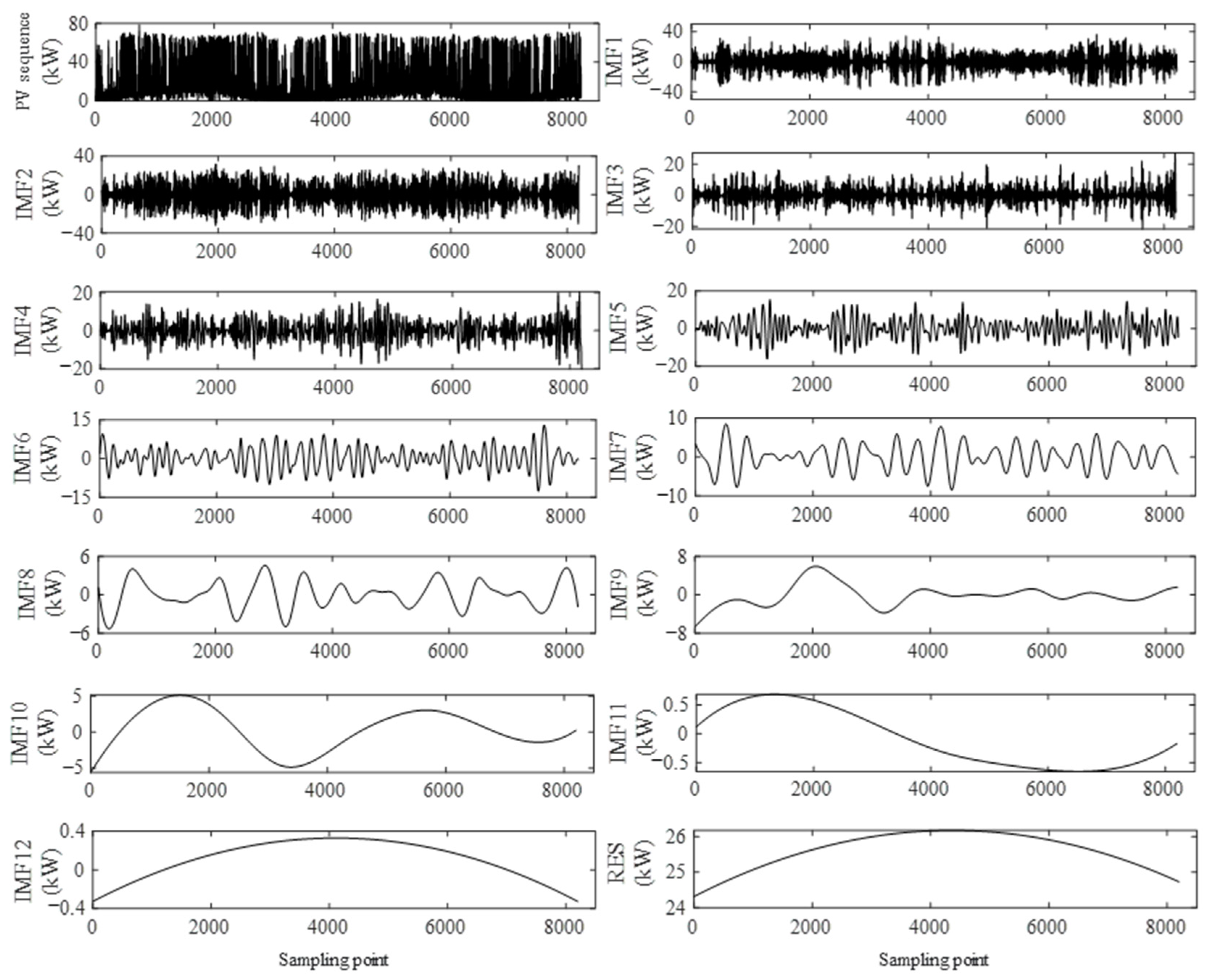
Perform EEMD decomposition on the original sequence set of historical PV power to obtain the corresponding IMF and residual components. The original power sequence and EEMD decomposition results are shown in Figure 3. This paper combines the experience of selecting parameters K and M in reference [32], and sets K = 0.1 and M = 100 in the experiment.
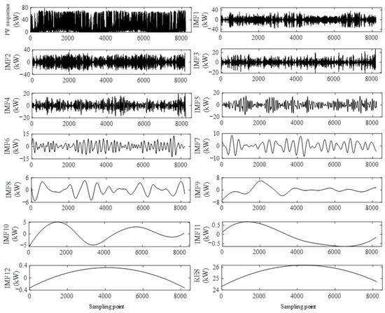
Figure 3.
EEMD decomposition of PV output sequence.
5.3. Component Merging Based on Amplitude Perception Permutation Entropy
AAPE is used to evaluate the complexity of IMF components and then the components with similar complexity are reconstructed to reduce computational complexity. The time delay has a small impact on the results, so usually taking = 1, and the embedding dimension m is determined by the pseudo neighbor method. In this paper, m = 5. The AAPE calculation results of the PV power sequence components are shown in Figure 4.
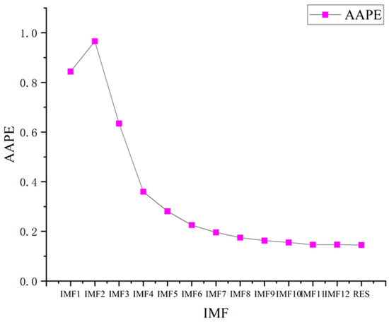
Figure 4.
AAPE values of PV power sequence components.
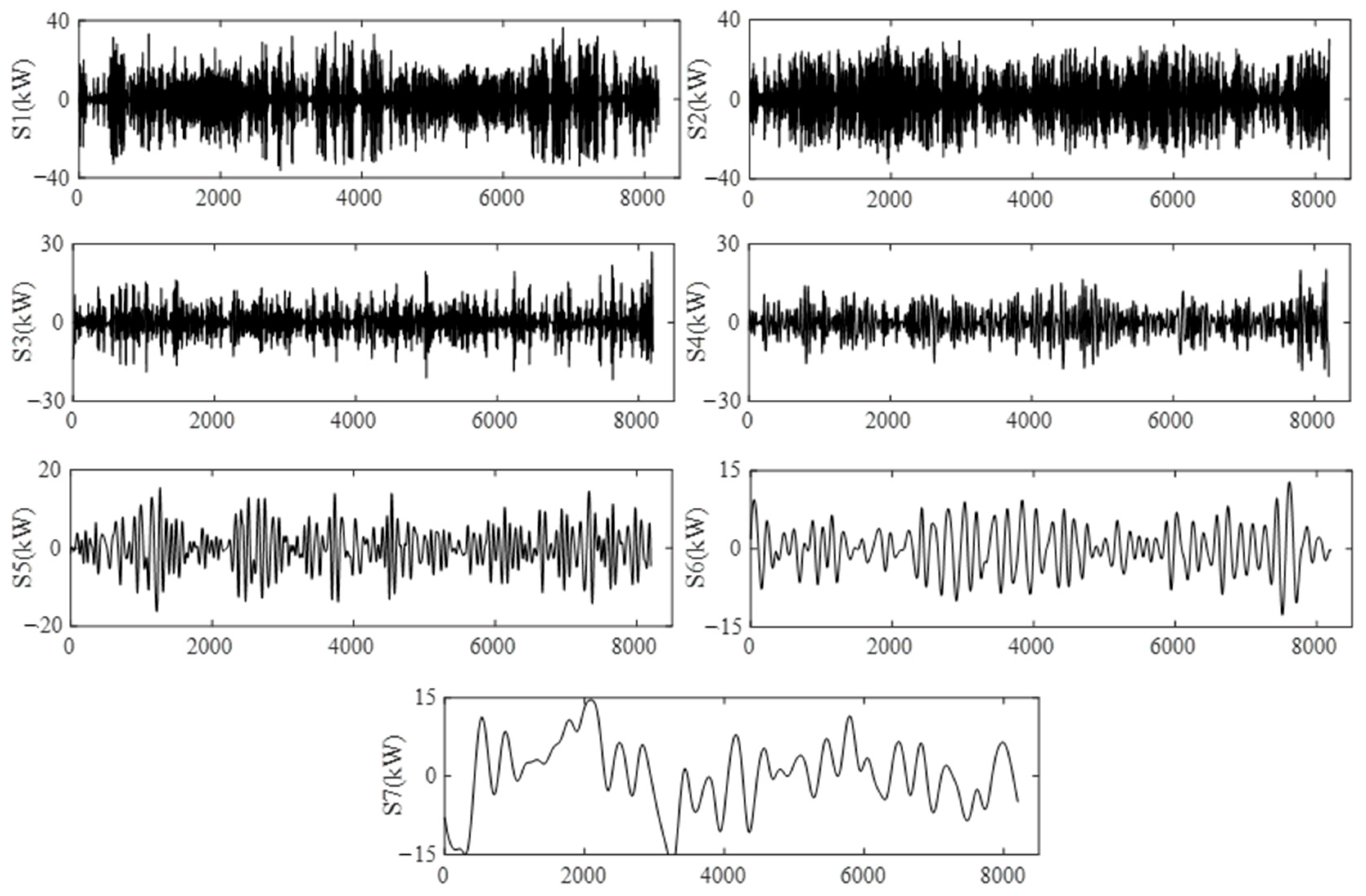
From Figure 4, it can be seen that the AAPE value of the high-frequency component of the original PV power sequence after decomposition is larger, indicating a higher complexity. The lower AAPE value of the low-frequency component indicates lower complexity. The AAPE values of the lower-frequency components, namely IMF7~IMF12, are very close, and the difference between adjacent components is less than 0.04 [33]. Therefore, these components are combined into a subsequence S6. The AAPE values of components IMF2~IMF6 differ significantly, so the original components remain unchanged and are, respectively, used as subsequences S1~S5. The residual components have a significant difference from adjacent components and are separately used as subsequences S7. The reconstructed subsequence is shown in Figure 5.
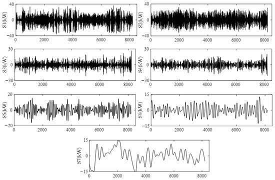
Figure 5.
Reconstructed sequence set based on AAPE.
5.4. Forecasting Model Parameters
In order to verify the effectiveness of the method proposed, two deep learning algorithms commonly used in time series prediction, graph convolutional networks (GCNs) and Long Short-Term Memory (LSTM), were also used for the simulation comparison verification.
Reasonable neural network parameter settings determine the reliability and accuracy of PV power sequence forecasting. The parameters of the GAT neural network constructed in this chapter are shown in Table 1, which includes one hidden layer and is trained 10 times. The batch size for each training is 64, with a time interval of 60, and the number of parallel working processes is 32. And parameters of the other models are shown in Table 2 and Table 3. This not only ensures the stability of model training, but also accelerates training speed and completes training better.

Table 1.
Parameters in the GAT neural network.
Table 2.
Parameters in the GCN.
Table 3.
Parameters in LSTM.
5.5. Analysis of Forecasting Results
To verify the effectiveness of introducing AAPE reconstruction and GAT neural networks in improving forecasting accuracy, EEMD-GCN-based models and EEMD-GAT-based models were constructed as comparative models. The above model parameters are consistent with the network parameters used in this paper. The error evaluation parameters are Relative Error, MAPE, and rRMSE as shown in Equations (18)–(20), respectively.
where represents the actual cumulative power generation value; represents the forecast cumulative power generation value; p represents the number of PV power sampling points in a day; represents the actual output of PV power on a certain day; represents the forecast output of PV power for that day. In the above indicators, relative error and MAPE, respectively, express the degree of deviation between cumulative days and specific daily forecast values and actual values, while rRMSE is highly sensitive to the error value of deviation from the mean in a certain group of forecast values. Table 4 and Table 5 present a comparison of the cumulative power generation forecasting values and forecasting errors for each forecasting model over a total of 15 days.
Table 4.
Results of PV output forecasting to dataset from HDU.
Table 5.
Results of PV output forecasting to dataset from the DKASC, Alice Springs.
From Table 4 and Table 5, it can be seen that in terms of the absolute value of cumulative forecast power generation, the forecast value of the method proposed in this paper is significantly closer to the actual value. From the perspective of relative error indicators, the proposed method in this paper has significantly lower Relative Error, MAPE, and rRMSE compared to the other two models. It can be seen that the model proposed in this paper has significantly improved learning ability and forecasting accuracy.
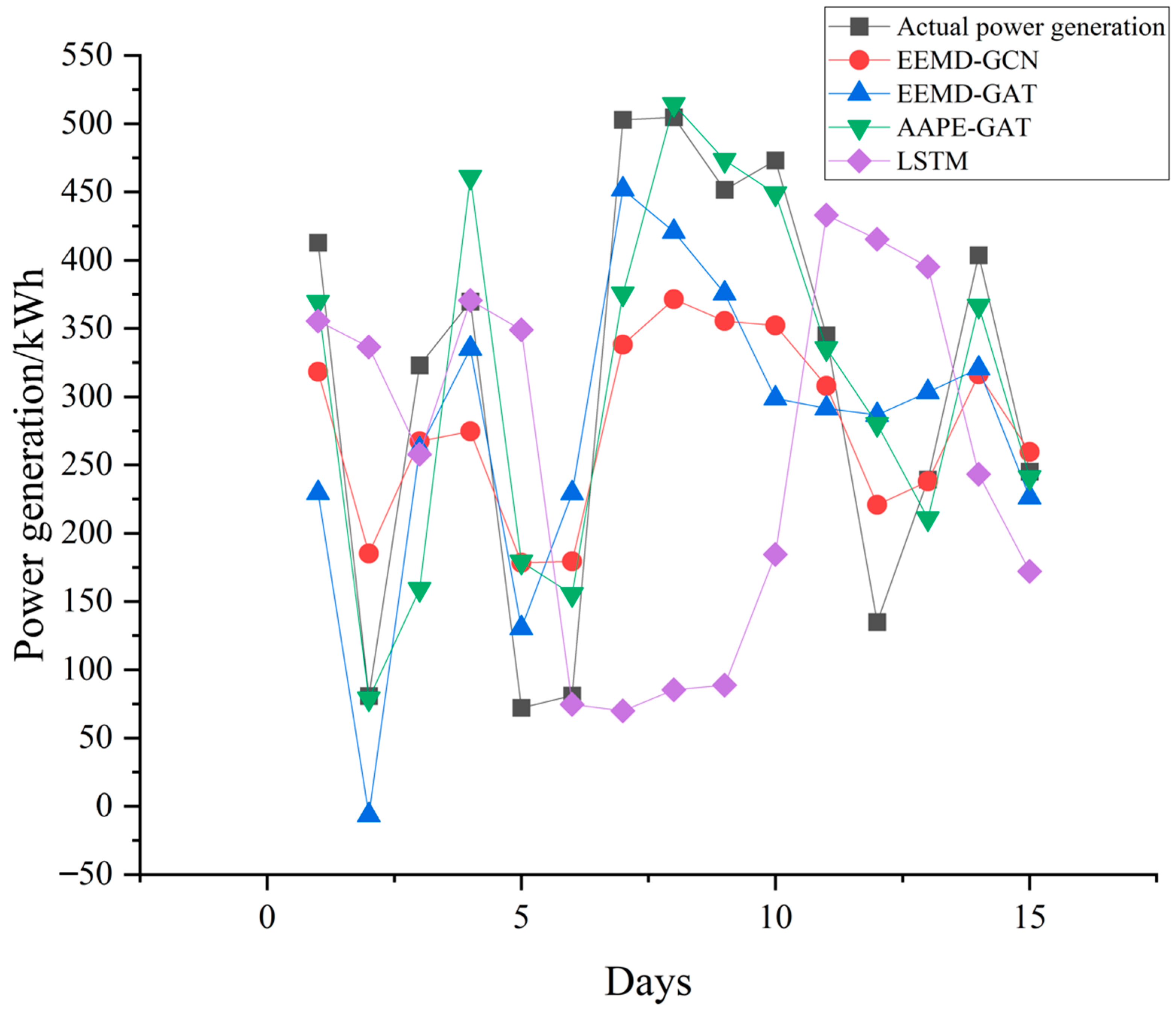
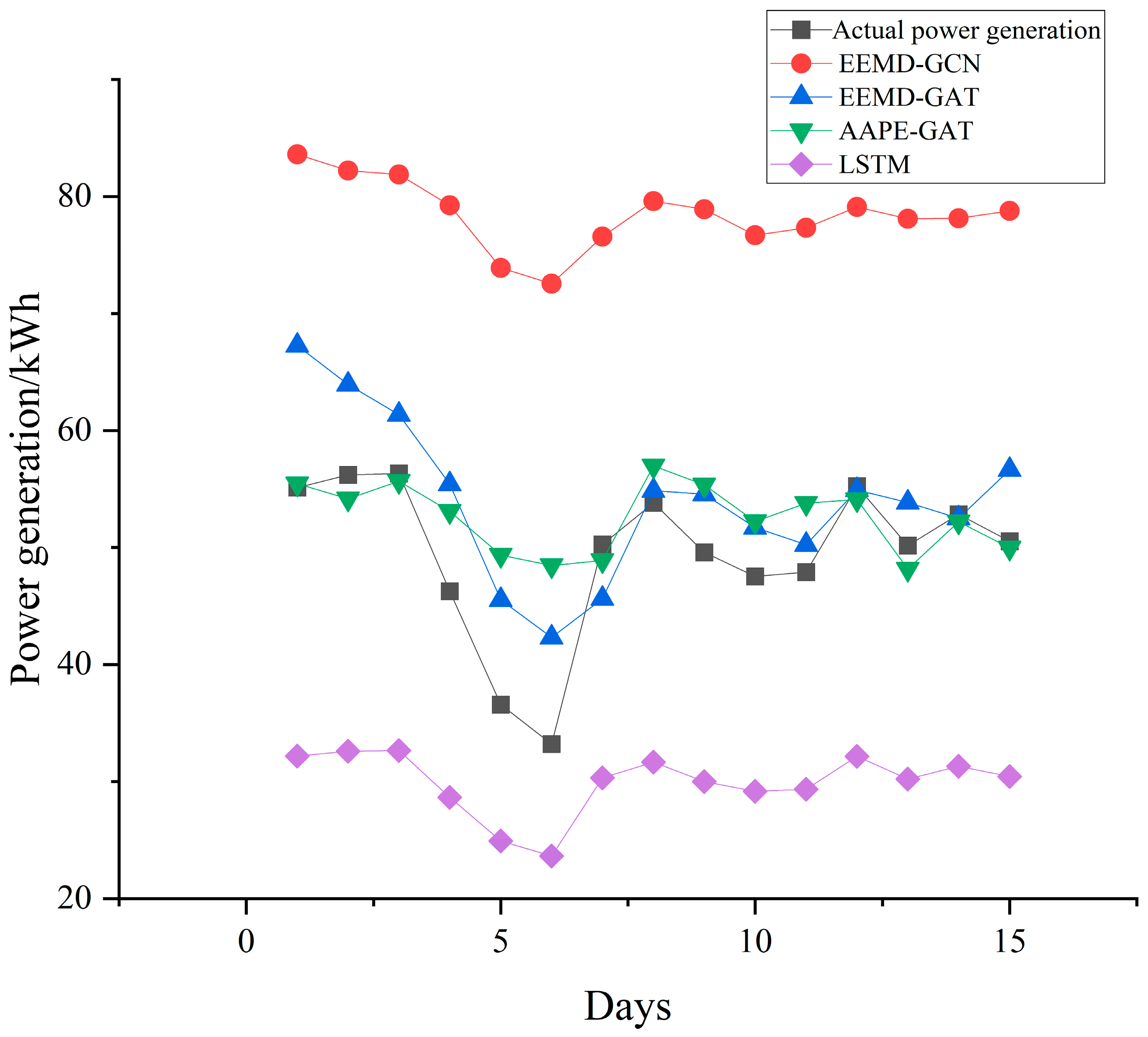
In addition, from the comparison of daily forecast power generation shown in Figure 6 and Figure 7, it can be seen that the method proposed in this paper has significantly more points similar to the actual power generation in the 15 day forecasting results than the other two models. Using GPU3060 (Colorful GeForce RTX 3060 DUO 12G, Hangzhou, China), the proposed model took only 8 min at training stage, and 2 min at testing stage. The comparison results are shown in Table 6. From Table 6, the running time is shorter and the calculation efficiency is higher than the other two networks.
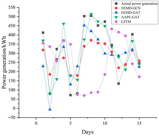
Figure 6.
Comparison of forecasted daily power generation to the dataset from HDU.
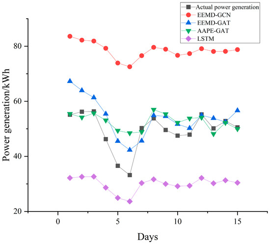
Figure 7.
Comparison of forecasted daily power generation to the dataset from the DKASC, Alice Springs.
Table 6.
Comparative results of different models’ running time.
This is because the use of the EEMD decomposition algorithm and the mutual information method improves the extraction of data features. In the forecasting process, the node adjacency matrix and reconstructed data can help the model better find the relationships between subsequences with similar features, improving the accuracy of PV sequence forecasting. The IMFs obtained by AAPE decomposition can capture the local change characteristics of the signal. These characteristics provide GAT with rich information and help to model and predict system behavior more accurately. In addition, the multi-scale signal features obtained by AAPE are combined with the attention mechanism of GAT to achieve cross-scale information fusion and improve the model’s ability to capture changes in different time scales. And the combined use of AAPE and GAT can resist the influence of noise interference and outliers to a certain extent, because both the decomposition process of AAPE and the attention mechanism of GAT have certain denoising capabilities. These are advantages that the compared models do not have.
6. Conclusions
This paper proposes a method for extracting data features based on the EEMD data decomposition method, AAPE and the mutual information method, as well as a PV output forecasting model using the GAT neural network. In this model, the PV power series data are first decomposed by EEMD to obtain IMF and residual components of different frequency components. Then, AAPE is calculated for the decomposed IMF and residual components, and the lower-complexity components are merged into a PV power subsequence. Afterwards, node feature sequences are obtained from each subsequence, and mutual information values are calculated for the node feature sequences. A calculation method for the node adjacency matrix is designed. Finally, a sequence of graph data is generated and the GAT neural network is used to obtain the forecasting results. The comparative experimental results show that the proposed model improves the forecasting accuracy in PV power sequence forecasting and can effectively forecasting medium–long-term PV power series. This method has certain practical application and promotion value. However, it should be noted that the proposed method requires a large amount of historical data for training, and is only suitable for PV power plants that have been built and operated for several years, because these power plants will have rich historical data. It is not applicable to new PV power stations, and one of the solutions is to use the transfer learning algorithm to establish the corresponding model by using the historical data of power stations with similar geographical locations.
Author Contributions
Conceptualization, S.S. and Y.H.; Methodology, G.C. and X.D.; Validation, G.C.; Data curation, X.D.; Writing—original draft, S.S.; Writing—review & editing, G.C.; Project administration, L.Z.; Funding acquisition, S.S. and Y.H. All authors have read and agreed to the published version of the manuscript.
Funding
This research was funded by [Science Foundation of State Grid Zhejiang Electric Power Co., Ltd.] grant number JY02202345.
Data Availability Statement
The original contributions presented in the study are included in the article, further inquiries can be directed to the corresponding authors.
Conflicts of Interest
Authors Shuyi Shen and Yingjing He are employed by the Economic Research Institute of State Grid Zhejiang Electric Power Company and declare that the company had no role in the design of the study; in the collection, analyses, or interpretation of data; in the writing of the manuscript; or in the decision to publish the results. The remaining authors declare that the research was conducted in the absence of any commercial or financial relationships that could be construed as a potential conflict of interest. The funder was not involved in the study design, collection, analysis, interpretation of data, the writing of this article or the decision to submit it for publication.
References
- Ding, S.; Li, R.; Tao, Z. A novel adaptive discrete grey model with time-varying parameters for long-term PV output forecasting. Energy Convers. Manag. 2021, 227, 113644. [Google Scholar] [CrossRef]
- Ranjan, K.G.; Prusty, B.R.; Jena, D. Review of preprocessing methods for univariate volatile time-series in power system applications. Electr. Power Syst. Res. 2021, 191, 106885. [Google Scholar] [CrossRef]
- Bauer, T.; Odenthal, C.; Bonk, A. Molten Salt Storage for Power Generation. Chem. Ing. Tech. 2021, 93, 534–546. [Google Scholar]
- Duan, C.; Fang, W.; Jiang, L.; Yao, L.; Liu, J. Distributionally Robust Chance-Constrained Approximate AC-OPF With Wasserstein Metric. IEEE Trans. Power Syst. 2018, 33, 4924–4936. [Google Scholar] [CrossRef]
- Cheng, H.; Cao, W.-S.; Ge, P.-J. Forecasting Research of Long-Term Solar Irradiance and Output Power for Photovoltaic Generation System. In Proceedings of the Fourth International Conference on Computational and Information Sciences, Kuala Terengganu, Malaysia, 7–8 March 2012; pp. 1224–1227. [Google Scholar] [CrossRef]
- Anggraeni, W.; Yuniarno, E.M.; Rachmadi, R.F.; Sumpeno, S.; Pujiadi, P.; Sugiyanto, S.; Santoso, J.; Purnomo, M.H. A hybrid EMD-GRNN-PSO in intermittent time-series data for dengue fever forecasting. Expert Syst. Appl. 2024, 237, 121438. [Google Scholar] [CrossRef]
- Li, Z.; Xu, R.; Luo, X.; Cao, X.; Du, S.; Sun, H. Short-term photovoltaic power prediction based on modal reconstruction and hybrid deep learning model. Energy Rep. 2022, 8, 9919–9932. [Google Scholar] [CrossRef]
- Hou, Z.; Zhang, Y.; Liu, Q.; Ye, X. A hybrid machine learning forecasting model for photovoltaic power. Energy Rep. 2024, 11, 5125–5138. [Google Scholar] [CrossRef]
- Sun, F.; Li, L.; Bian, D.; Ji, H.; Li, N.; Wang, S. Short-term PV power data prediction based on improved FCM with WTEEMD and adaptive weather weights. J. Build. Eng. 2024, 90, 109408. [Google Scholar] [CrossRef]
- Feng, H.; Yu, C. A novel hybrid model for short-term prediction of PV power based on KS-CEEMDAN-SE-LSTM. Renew. Energy Focus 2023, 47, 100497. [Google Scholar] [CrossRef]
- Netsanet, S.; Zheng, D.; Zhang, W.; Teshager, G. Short-term PV power forecasting using variational mode decomposition integrated with Ant colony optimization and neural network. Energy Rep. 2022, 8, 2022–2035. [Google Scholar] [CrossRef]
- Li, Y.; Wang, X.; Liu, Z.; Liang, X.; Si, S. The Entropy Algorithm and Its Variants in the Fault Diagnosis of Rotating Machinery: A Review. IEEE Access 2018, 6, 66723–66741. [Google Scholar] [CrossRef]
- Yang, M.; Huang, Y.; Guo, Y.; Zhang, W.; Wang, B. Ultra-short-term wind farm cluster power prediction based on FC-GCN and trend-aware switching mechanism. Energy 2024, 290, 130238. [Google Scholar] [CrossRef]
- Liu, X.; Yu, J.; Gong, L.; Liu, M.; Xiang, X. A GCN-based adaptive generative adversarial network model for short-term wind speed scenario prediction. Energy 2024, 294, 130931. [Google Scholar] [CrossRef]
- Zhao, J.; Yan, Z.; Chen, X.; Han, B.; Wu, S.; Ke, R. k-GCN-LSTM: A k-hop Graph Convolutional Network and Long–Short-Term Memory for ship speed prediction. Phys. A Stat. Mech. Its Appl. 2022, 606, 128107. [Google Scholar] [CrossRef]
- Mansoor, H.; Gull, M.S.; Rauf, H.; Shaikh, I.U.H.; Khalid, M.; Arshad, N. Graph Convolutional Networks based short-term load forecasting: Leveraging spatial information for improved accuracy. Electr. Power Syst. Res. 2024, 230, 110263. [Google Scholar] [CrossRef]
- Giamarelos, N.; Zois, E.N. Boosting short term electric load forecasting of high & medium voltage substations with visibility graphs and graph neural networks. Sustain. Energy Grids Netw. 2024, 38, 101304. [Google Scholar] [CrossRef]
- Xia, Z.; Zhang, Y.; Yang, J.; Xie, L. Dynamic spatial–temporal graph convolutional recurrent networks for traffic flow forecasting. Expert Syst. Appl. 2024, 240, 122381. [Google Scholar] [CrossRef]
- Velickovic, P.; Cucurull, G.; Casanova, A.; Romero, A.; Lio, P.; Bengio, Y. Graph attention networks. Stat 2017, 1050, 10-48550. [Google Scholar]
- Zhao, J.; Yan, Z.; Zhou, Z.; Chen, X.; Wu, B.; Wang, S. A ship trajectory prediction method based on GAT and LSTM. Ocean Eng. 2023, 289, 116159. [Google Scholar] [CrossRef]
- Lin, S.; Wang, S.; Xu, X.; Li, R.; Shi, P. GAOformer: An adaptive spatiotemporal feature fusion transformer utilizing GAT and optimizable graph matrixes for offshore wind speed prediction. Energy 2024, 292, 130404. [Google Scholar] [CrossRef]
- Sang, W.; Zhang, H.; Kang, X.; Nie, P.; Meng, X.; Boulet, B.; Sun, P. Dynamic multi-granularity spatial-temporal graph attention network for traffic forecasting. Inf. Sci. 2024, 662, 120230. [Google Scholar] [CrossRef]
- Ge, Z.; Xu, X.; Guo, H.; Wang, T.; Yang, Z. Speaker recognition using isomorphic graph attention network based pooling on self-supervised representation. Appl. Acoust. 2024, 219, 109929. [Google Scholar]
- Wang, P.-H.; Zhu, Y.-H.; Yang, X.; Yu, D.-J. GCmapCrys: Integrating graph attention network with predicted contact map for multi-stage protein crystallization propensity prediction. Anal. Biochem. 2023, 663, 1150520. [Google Scholar] [CrossRef]
- Wang, S.; Yang, Z.; Zheng, X.; Ma, Z. Analysis of complex time series based on EEMD energy entropy plane. Chaos Solitons Fractals 2024, 182, 114866. [Google Scholar] [CrossRef]
- Azami, H.; Escudero, J. Amplitudeaware permutation entropy: Illustration in spike detection and signal segmentation. Comput. Methods Programs Biomed. 2016, 128, 40–51. [Google Scholar] [CrossRef]
- Vaswani, A.; Shazeer, N.; Parmar, N.; Uszkoreit, J.; Jones, L.; Gomez, A.N.; Kaiser, L.; Polosukhin, I. Attention is all you need. Adv. Neural Inf. Process. Syst. 2017, 30. [Google Scholar] [CrossRef]
- Liu, J.; Li, T. Multi-step power forecasting for regional photovoltaic plants based on ITDE-GAT model. Energy 2024, 293, 130468. [Google Scholar] [CrossRef]
- Wang, F.; Yang, J.-F.; Wang, M.-Y.; Jia, C.-Y.; Shi, X.-X.; Hao, G.-F.; Yang, G.-F. Graph attention convolutional neural network model for chemical poisoning of honey bees’ prediction. Sci. Bull. 2020, 65, 1184–1191. [Google Scholar] [CrossRef]
- Bahdanau, D.; Cho, K.; Bengio, Y. Neural machine translation by jointly learning to align and translate. In Proceedings of the International Conference on Learning Representations (ICLR), San Diego, CA, USA, 7–9 May 2015. [Google Scholar]
- Zhou, L.; Wang, H. MST-GAT: A multi-perspective spatial-temporal graph attention network for multi-sensor equipment remaining useful life prediction. Inf. Fusion 2024, 110, 102462. [Google Scholar] [CrossRef]
- Durrani, S.P.; Balluff, S.; Wurzer, L.; Krauter, S. Photovoltaic yield prediction using an irradiance forecast model based on multiple neural networks. J. Mod. Power Syst. Clean Energy 2018, 6, 255–267. [Google Scholar] [CrossRef]
- Almonacid, F.; Pérez-Higueras, P.; Fernández, E.F.; Hontoria, L. A methodology based on dynamic artificial neural network for short-term forecasting of the power output of a PV generator. Energy Convers. Manag. 2014, 85, 389–398. [Google Scholar] [CrossRef]

Disclaimer/Publisher’s Note: The statements, opinions and data contained in all publications are solely those of the individual author(s) and contributor(s) and not of MDPI and/or the editor(s). MDPI and/or the editor(s) disclaim responsibility for any injury to people or property resulting from any ideas, methods, instructions or products referred to in the content. |
© 2024 by the authors. Licensee MDPI, Basel, Switzerland. This article is an open access article distributed under the terms and conditions of the Creative Commons Attribution (CC BY) license (https://creativecommons.org/licenses/by/4.0/).