Capacity Demand Analysis of Rural Biogas Power Generation System with Independent Operation Considering Source-Load Uncertainty

Abstract

With the greatly increased penetration rate of wind power, photovoltaic, and other new energy sources in the power system, the proportion of controllable units gradually decreased, resulting in increased system uncertainty. The biogas power generation system can effectively alleviate the pressure caused by source-load uncertainty in such high-permeability systems of new energy sources such as wind power and photovoltaic. Hence, from the perspective of the power system, this paper introduces a capacity demand analysis method for a rural biogas power generation system capable of independent operation amidst source-load uncertainty. To enhance the depiction of pure load demand uncertainty, a scene set generation method is proposed, leveraging quantile regression analysis and Gaussian mixture model clustering. Each scene’s data and probability of occurrence elucidate the uncertainty of pure load demand. An integrated optimal operation model for new energy and biogas-generating units, free from energy storage capacity constraints, is established based on the generated scenario set. Addressing considerations such as biogas utilization rate and system operation cost, a biogas storage correction model, utilizing the gas storage deviation degree index and the cost growth rate index, is developed to determine biogas demand and capacity. The example results demonstrate the significant reduction in gas storage construction costs and charging and discharging imbalances achieved by the proposed model while ensuring systemic operational cost effectiveness.

1. Introduction

In the low-carbon context, the penetration rate of new energy (such as wind power, photovoltaic, and other distributed generators) in the latest power system has increased significantly, increasing the power system’s uncertainty [1]. As a high-quality, flexible resource, biogas’s participation in rural microgrids can effectively improve the system’s ability to cope with uncertainty [2]. With the support of relevant policies, biogas generators have been widely used in rural distribution networks, mainly focusing on scenarios such as stabilizing station output fluctuations and improving the schedulability of new energy sources [3,4]. The service object of biogas generators is the station, and its capacity requirements under the rural power grid that can operate independently are considered to a lesser degree. It is not easy to fully play the role of biogas, and the configuration of biogas generators can make up for the above deficiencies and has a good economy [5,6]. Therefore, it is of great theoretical significance and application value to evaluate the demand capacity of biogas-generating units from the system-level perspective in the face of the increasingly severe, new energy, high-permeability system and the low economy of the biogas power generation system.

In Reference [7], the uncertainty of wind, light, and load forecasting errors is characterized using the Gaussian random distribution probability model. Meanwhile, in [8], the uncertainty of load is depicted using the standard distribution model, while the randomness of the photovoltaic system is described using the Beta distribution model. The above research is based on the parameter probability prediction model to characterize the uncertainty, but the error is significant, and the applicability is poor. In this regard, Reference [9] proposed a fuzzy set construction method of wind power probability distribution based on principal component analysis and kernel density estimation, which effectively characterized the uncertainty of wind power output. In Reference [10], a scenario integration method of new energy combined output is proposed by coupling quantile regression analysis (QRA) and dimensionality reduction clustering technology, which is used to describe the uncertainty of new energy output. Reducing the dimension of the data is a common strategy employed in these scenarios, aimed at streamlining the calculation process. However, this approach raises concerns regarding the integrity of the data, as it may compromise certain aspects of the information.

Significant progress has also been made in analyzing optimized capacity requirements at home and abroad. Reference [11] considers adding energy storage in renewable energy power generation systems to minimize power generation costs by optimizing the capacity configuration of energy storage and renewable energy. References [12,13] evaluates the impact of increasing energy storage on the economy, energy efficiency, and environment based on the existing distributed generation. Studies have shown that increasing energy storage can reduce system and environmental costs. In Reference [14], considering the energy storage system’s investment cost and economic benefit, the optimal value of energy storage capacity allocation is obtained by a genetic algorithm, with annual income maximization as the objective function. In References [15,16], the influence of demand response on microgrid systems’ capacity configuration and economy under off-grid and grid-connected conditions are studied, respectively. In Reference [17], a bi-objective optimization model is established with minimum annual total planning cost and minimum annual carbon dioxide emissions considering demand response. The results show that considering demand response can reduce system configuration costs and carbon emissions. However, the above research takes energy storage as the research goal, and the investment cost of energy storage is high, which makes it difficult to be widely applied in rural power grids. In rural power grids with abundant biogas resources, the research on using biogas generators to improve the regulation ability of rural power grids has become a hot spot. The biogas power generation system should be taken as the research object, and the capacity demand analysis of the biogas power generation system should be carried out to ensure stable operation.

In this paper, the capacity demand analysis method of the biogas power generation system is studied for the rural power grid, which can operate independently under the uncertainty of source and load. Firstly, to analyze the source-load uncertainty reasonably, the scenario set generation method based on QRA and Gaussian mixture model (GMM) is used to describe the uncertainty of pure load demand accurately.

Furthermore, leveraging the characterization results, an optimal operation model for the system, incorporating biogas-generating units, is formulated. Subsequently, a power correction model for the biogas generator set is devised to ensure that the adjusted gas storage capacity accounts for both biogas utilization rate and system operation cost. Ultimately, building upon these developments, the demand capacity of the biogas power generation system is determined.

2. Source-Load Uncertainty Analysis of Rural Distribution Network

The uncertainty of source and load increases the difficulty of rural power grid dispatching, and biogas-generating units can effectively control the uncertainty of the system. Therefore, the capacity demand analysis of rural biogas power generation systems should be based on system uncertainty. Thus, this paper uses the typical scenario set of pure load demand (the difference between the actual load of the system and the total output of new energy) to characterize the system uncertainty and provide a basis for analyzing the capacity of energy storage demand.

2.1. Pure Load Demand Sample Processing Based on QRA

The uncertainty of pure load demand is reflected in the uncertainty of the error between the predicted power and the actual power, which has the characteristics of a large amount of data and information. QRA can fully tap the valuable information of a large amount of data. It is easy to describe the various occurrences of the actual power of the pure load demand according to the pure load demand forecast power. Therefore, this paper uses QRA to process the pure load demand samples.

Let the probability of the random variable $y\le y_{\tau }$ be τ, and then, y is defined as the τ quantile of y, as given below:

$$y_{\tau }=\left\{y|F\left(y\right)\le \tau \right\}$$

(1)

where $F\left(y\right)$ is the probability distribution function of the random variable y.

The actual power matrix and the predicted power matrix of the pure load demand of the new energy, high-permeability system are set as $P_{\mathrm{r}}$ and $P_{\mathrm{f}}$, respectively, and $p_{\mathrm{r}}\left(i,j\right)$ and $p_{\mathrm{f}}\left(i,j\right)$ are the ith row and jth column elements of $P_{\mathrm{r}}$ and $P_{\mathrm{f}}$, respectively, which represent the jth sampling point of the actual power and the predicted power of the pure load demand on the ith day, respectively. In the case of τ quantile, the linear mapping relationship between the exact power and the expected power fitted by quantile regression is as follows:

$$p_{\mathrm{r},\tau }\left(i,j\right)=a_{\tau }{p}_{\mathrm{f}}\left(i,j\right)+b_{\tau }$$

(2)

where $a_{\tau }$ and $b_{\tau }$ are the parameter values of the linear fitting curve under the actual power $p_{\mathrm{r},\tau }\left(i,j\right)$ of the τ quantile netload.

The estimation of the fitting curve parameters $a_{\tau }$ and $b_{\tau }$ can be obtained by (3).

$$\min \hspace{0.33em}Q\left(\tau \right)={\displaystyle \sum _{i=1}^I{\displaystyle \sum _{j=1}^J{f}_{\tau }\left[p_{\tau }\left(i,j\right)-p_{\mathrm{r},\tau }\left(i,j\right)\right]}}$$

(3)

$$f_{\tau }\left(x\right)=\left\{\begin{array}{cc}\tau x,\hfill & \hfill x\ge 0\\ \left(\tau -1\right)x,\hfill & \hfill x<0\end{array}\right.$$

(4)

where $Q\left(\tau \right)$ is the τ quantile objective function, and $f_{\tau }\left(x\right)$ is the test function. I and J are the total number of scenarios and daily sampling points of the pure load demand samples, respectively.

Different τ values can obtain different $a_{\tau }$ and $b_{\tau }$. For the same pure load demand forecasting power $p_{\mathrm{f}}$, a set of pure load demand actual power quantiles can be obtained, where ${\tau }_1$, ${\tau }_2$, …, ${\tau }_O$ are the different quantiles.

2.2. GMM-Based Source-Load Uncertainty Clustering

The daily pure load demand sequence is high-dimensional data with many scene sets and complicated calculations. In this paper, GMM, which has a solid ability to describe high-dimensional data, high clustering accuracy, and good robustness, is used for scene clustering, aiming to reduce the computational complexity.

The pure load demand data is partitioned into k categories, represented by the k components of the GMM. The probability associated with each pure load demand data point can be expressed as follows:

$$p\left(x\right)={\displaystyle \sum _{i=1}^k{\omega }_{i}p\left(x|{\mu }_i,{\sum }_i\right)}$$

(5)

where $p\left(x\right)$ is the probability of each pure load demand data; ${\omega }_i$ is the weight coefficient of the ith Gaussian distribution component; and $p\left(x|{\mu }_i,{\sum }_i\right)$ is the probability density function of the Gaussian distribution with mean value ${\mu }_i$ and covariance ${\sum }_i$. ${\mu }_i$ and ${\sum }_i$ are the mean value and covariance of the ith Gaussian distribution component, respectively.

The objective function can be expressed as follows:

$$\max \hspace{0.33em}{\displaystyle \sum \lg \hspace{0.33em}p\left(x\right)}={\displaystyle \sum \lg \left[{\displaystyle \sum _{i=1}^k{\omega }_{i}p\left(x|{\mu }_i,{\sum }_i\right)}\right]}$$

(6)

2.3. System Typical Scene Generation

The typical scenario set of pure load demand can better describe the uncertainty of pure load demand. The pure load demand used in this paper is used to generate the typical scenario set. The specific steps are as follows:

(1)

According to the QRA, the nonparametric probability prediction model is determined, and the quantile $\left\{{\tau }_{i,j}|i=1,2,\cdots ,J\right\}$ corresponding to the actual power $p_{\tau }\left(i,j\right)$ of the historical pure load demand is obtained by interpolation calculation.

(2)

Let $T_{i,j}=\left[{\tau }_{i,j}\right]$, the probit function, be used to transform $T_{i,j}$ which obeys uniform distribution in I, and this obeys J-dimensional Gaussian distribution $N_J\left(\mu ,\sum \right)$ ($\mu$, Σ are parameters of multivariate Gaussian distribution), and the maximum likelihood estimation is the sample mean vector $\overline{X}$ and the sample covariance matrix S.

(3)

Based on the GMM clustering method, I pure load demand scenarios are reduced to k typical pure load demand scenarios, and their distribution probability ${\rho }_{k,\mathrm{typ}}$ is obtained.

(4)

The probit inverse function is used to transform k vectors obeying the J-dimensional Gaussian distribution into k vectors obeying the uniform distribution $T_J={\left[{\tau }_{s,1},{\tau }_{s,2},\cdots ,{\tau }_{s,J}\right]}^{\mathrm{T}}$, where $s=1,2,\cdots ,k$. $\left(J=1,2,\cdots ,J\right)$ are the quantiles of the jth sampling point of the typical pure load demand scenario s.

(5)

The non-parametric model is used to obtain the quantile matrix $P_{\mathrm{r},\tau }$ of the known pure load demand forecasting power. Then, the matrix composed of k quantile vectors $T_J$ is linearly interpolated according to $P_{\mathrm{r},\tau }$, to obtain k pure load demand typical scenario sets $P_{k,\mathrm{typ}}$ corresponding to the pure load demand forecasting power sequence, as shown in (7).

$$P_{k,\mathrm{typ}}=\left[\begin{array}{c}{\left[p_{\mathrm{r},1,1},p_{\mathrm{r},1,2},\cdots p_{\mathrm{r},1,J}\right]}^{\mathrm{T}}\\ {\left[p_{\mathrm{r},2,1},p_{\mathrm{r},2,2},\cdots p_{\mathrm{r},2,J}\right]}^{\mathrm{T}}\\ ⋮\\ {\left[p_{\mathrm{r},k,1},p_{\mathrm{r},k,2},\cdots p_{\mathrm{r},k,J}\right]}^{\mathrm{T}}\end{array}\right]$$

(7)

$${\rho }_{k,\mathrm{typ}}={\left[{\rho }_1,{\rho }_2,\cdots ,{\rho }_k\right]}^{\mathrm{T}}$$

(8)

where ${\left[p_{\mathrm{r},i,1},p_{\mathrm{r},i,2},\cdots p_{\mathrm{r},i,J}\right]}^{\mathrm{T}}\left(i=1,2,\cdots ,k\right)$ is the pure load demand power vector of the ith pure load demand scenario, and ${\rho }_i$ is the distribution probability of the ith pure load demand scenario.

3. Optimized Operation Model of Rural Microgrid Based on Source-Load Uncertainty

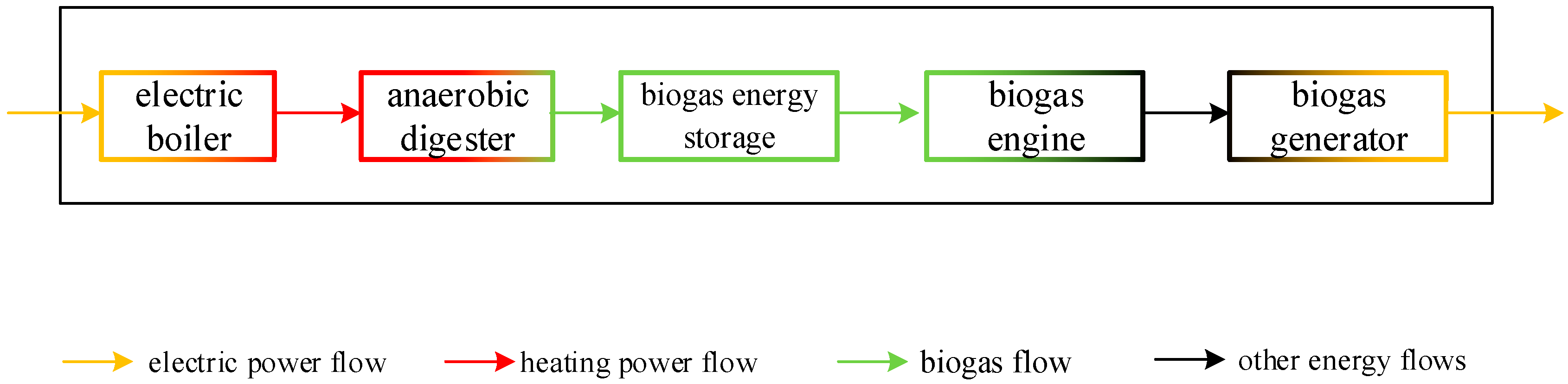
3.1. Rural Biogas Power Generation System Model

3.1.1. Biogas Fermentation Kinetic Model

Microbial kinetics mainly refers to the basic theory and experimental methods of chemical reaction kinetics and enzyme-catalyzed reaction kinetics. It studies the kinetic characteristics of microbial growth, substrate consumption, and product formation at various levels of microbial molecules or enzymes, cells, microbial populations, and bioreactors. These micro-level microbial reaction kinetics characteristics will be reflected in the complex, large-scale biological processes at the macro level, and the modeling methods for describing the complex, large-scale biological processes at the macro level mainly include derivation from the micro-dynamics that reflects the reaction metabolism mechanism, fitting the experimental curve with pure mathematical method; the non-structural model is analogized by the formal dynamic method. Among them, the third unstructured model is based on the steady-state hypothesis and the theory of microbial metabolic reaction, ignoring the microscopic changes in microbial cell components, and using the experimental curve fitting results as model parameters. It has the advantages of the first and second methods and is widely used to describe the complex, large-scale microbial reaction process. Therefore, in this section, the non-structural model based on the Monod equation is used to describe the steady-state approximate relationship between biogas fermentation rate and different environmental factors under medium temperature or room temperature, such as substrate concentration, strain type (biomass raw material), temperature, and so on. Therefore, the kinetic model of biogas fermentation is as shown in Equations (9)–(11):

$${\mu }_t^d=\left\{\begin{array}{l}{\alpha }_{11}{e}^{{\alpha }_{12}{T}_t^d},\hspace{0.33em}\hspace{0.33em}\hspace{0.33em}\hspace{0.33em}{T}_0-T_1\\ {\alpha }_{21}{T}_t^d-{\alpha }_{22},\hspace{0.33em}\hspace{0.33em}\hspace{0.33em}{T}_1-T_2\end{array}\right.$$

(9)

$$K^d={\beta }_{11}{e}^{{\beta }_{12}{S}_0}+{\beta }_{13}$$

(10)

$$G_t=\frac{B_0{S}_0{V}_{AD}}{24\cdot HRT}\left(1-\frac{K^d}{HRT\cdot {\mu }_t^d-1+K^d}\right)$$

(11)

where ${\mu }_t^d$ is the maximum growth rate of bacterial biomass at t under medium- or low-temperature conditions, and its dimension is kg/h; $G_t$ is the biogas (methane) yield of the biogas generator set at t, and its dimension is m³/kg; $B_0$ is the biological methane potential, indicating how much organic matter can be degraded in the anaerobic reaction, and its dimension is m³/kg; and $S_0$ is the quality of volatile solids (VS) in the fermentation base liquid of anaerobic digester (AD), and its dimension is kg. Volatile solids refer to the amount of organic matter removed from the inorganic part of the total solids, which is the most critical practical component of microbial fermentation. $V_{AD}$ is the AD volume of the anaerobic tank t, and its dimension is m³; $K^d$ is the kinetic parameter of microbial fermentation; HRT is hydraulic retention time, that is, the average reaction time of microbial fermentation, and its dimension is h; ${\alpha }_{11}$, ${\alpha }_{12}$, ${\alpha }_{21}$, ${\alpha }_{22}$, ${\beta }_{11}$, ${\beta }_{12}$, and ${\beta }_{13}$ are microbial fermentation coefficients, which are related to the type of biomass raw materials and fermentation methods, and are generally obtained by experimental fitting, and their values in this paper are 0.004, 2.5, 0.5, 0.15, 0.3, and 0.65.

3.1.2. Biogas Power Generation Model

As shown in Figure 1, biogas generator sets usually comprise pretreatment equipment, AD, biogas energy storage (BES), and biogas generator sets. The collected biomass raw materials are pretreated and mixed with water as the fermentation base liquid. The excess biogas is produced by AD fermentation and stored in BES. When there is a power shortage in the distribution network, the biogas generator sets provide system support services by burning the stored biogas to generate electricity. The waste heat recovery and electric heating of the biogas generator set act on AD simultaneously, increasing and maintaining the fermentation temperature, promoting the microbial metabolic rate, and increasing biogas production. The gas production, storage, and consumption process make the biogas generator set complete the mutual conversion of different energy forms. Equations (11)–(26) model the gas production, storage, and consumption processes reflected above, respectively.

(12)–(15) represent the heat conduction process during the fermentation gas production. The total heat energy for heating AD comes from the heat recovery of the biogas generator set and the electric heating equipment. According to the law of steady-state heat conduction, (14) represents the total heat dissipated by the surface, such as AD’s top and side walls. According to the law of conservation of energy, (15) indicates that the fermentation temperature in AD changes with heat balance.

$$H_t^{AD}=\left(H_t^{\mathrm{grid}}+H_t^{\mathrm{LBP}}\right),\forall t$$

(12)

$$H_t^{\mathrm{grid}}={\eta }_e{P}_t^{\mathrm{grid}},\forall t$$

(13)

$$H_t^{dis}=K^{dis}{A}_{air-AD}\left(T_t-T_t^{air}\right)$$

(14)

$$T_{t+1}=T_t+\frac{\left(H_t^{grid}+H_t^{AD}-H_t^{dis}\right)\cdot \Delta t}{c_{AD}{\rho }_{AD}{V}_{AD}},\forall t$$

(15)

where $H_t^{AD}$ is the total thermal power of heating AD fermentation base fluid at t, and its dimension is kW; $H_t^{\mathrm{grid}}$ is the output power of the electric heating equipment at t, and its dimension is kW; $H_t^{\mathrm{LBP}}$ is the thermal power of biogas generator set at t, and its dimension is kW; ${\eta }_e$ is the electrothermal conversion efficiency of electric heating equipment; $P_t^{\mathrm{grid}}$ is the power of electric heating equipment at t, and its dimension is kW; $H_t^{dis}$ is the heat dissipation power transmitted through the surface of the AD tank wall, and its dimension is kW; $K^{dis}$ is the heat transfer coefficient of the AD pool wall; $A_{air-AD}$ is the surface area of AD pool wall, and its dimension is m³; $T_t$ is the fermentation temperature in the pool at t, and its dimension is °C; $T_t^{air}$ is the ambient temperature at t, and its dimension is °C; $c_{AD}$ and ${\rho }_{AD}$ are the specific heat capacity and density of the fermentation broth, and their dimensions are J/(kg·°C) and kg/m³, respectively.

In the gas storage stage, the biogas produced by fermentation is first transported to the gas storage tank for storage. In most biogas-generating units, the AD outlet pipe is directly connected to the BES inlet pipe. Therefore, the BES inlet rate is equal to the biogas fermentation rate, and the BES outlet rate is equal to the inlet rate of the biogas-generating unit. Equation (16) indicates that the gas storage capacity in BES varies with the inlet and outlet rates, and Equation (17) indicates that the maximum capacity of BES limits the gas storage capacity. Equation (18) limits the maximum outgassing rate of BES, that is, the intake rate of the biogas generator set. To ensure the sustainable operation of the biogas generator set, the gas storage state of the gas storage tank in the last period of each day must be not less than the initial gas storage value, as shown in Equation (19).

$$G_{t+1}^{BES}=G_t^{BES}+{\eta }_{BES}{G}_t-\frac{G_t^{LBP}}{{\eta }_{BES}},\forall t$$

(16)

$${\underset{\_}{G}}_t^{BES}\le G_t^{BES}\le {\overline{G}}^{BES},\forall t$$

(17)

$$0\le G_t^{LBP}\le {\overline{G}}^{LBP},\forall s,\forall t$$

(18)

$$G_{t=24}^{BES}\ge G_{t=0}^{BES}$$

(19)

where $G_t^{BES}$ is the gas storage capacity of BES at t, and its dimension is m³; ${\overline{G}}^{BES}$ is the maximum intake rate of the Large-scaled Biogas Plant (LBP) unit, and its dimension is m³/h; ${\eta }_{BES}$ is the charging and discharging efficiency of BES; $G_t^{LBP}$ is the intake rate of biogas generator set at t, and its dimension is m³/h.

In the gas phase, according to the law of energy conservation, the intake rate of the biogas generator set limits the total output power of the biogas generator set, as shown in (12). The heat-to-electricity ratio of the biogas generator set should meet the constraints of its operational feasible region. An auxiliary variable $y_{tn}$ is introduced here. Assuming that $\left(P_n^{LBP},H_n^{LBP}\right)$ represents the set of thermal and electrical power at the nth pole in its operational feasible region, the electrical and thermal power of the biogas generator set at t can be expressed by Equations (20)–(24). The Equations (25) and (26) indicate the upper and lower limits of the biogas generator’s thermal and electrical power climbing rate.

$$H_t^{LBP}+P_t^{LBP}={\eta }_{con}\cdot G_t^{LBP},\forall t$$

(20)

$$P_t^{LBP}=\sum _{n\in SN}{\gamma }_{tn}\cdot P_n^{LBP},\forall t$$

(21)

$$H_t^{LBP}=\sum _{n\in SN}{\gamma }_{tn}\cdot H_n^{LBP},\forall t$$

(22)

$$\sum _{n\in SN}{y}_{tn}=1,\forall t$$

(23)

$$0\le y_{tn}\le 1,\forall n\in SN,\forall t$$

(24)

$$-H^{down}\le H_{t+1}^{LBP}-H_t^{LBP}\le H^{up},\forall t$$

(25)

$$-P^{down}\le P_{t+1}^{LBP}-P_t^{LBP}\le P^{up},\forall t$$

(26)

where $y_{tn}$ is the auxiliary variable, and the operating state of the biogas generator set is constrained within its feasible region. $H^{up}$ and $H^{down}$ are the upper and lower limits of thermal power climbing of biogas power generation, and their dimension is kW; $P^{up}$ and $P^{down}$ are the upper and lower limits of biogas power climbing, and their dimension is kW, respectively. $P_t^{LBP}$ is the active output power of the biogas generator set at t, and its dimension is kW; ${\eta }_{con}$ is the energy conversion efficiency of the biogas generator set; SN is the collection of all poles in the feasible region of the biogas generator set operation. The gas production, gas storage, and gas consumption process enable the biogas generator set to absorb the excess electric energy in the distribution network through electric heating equipment and produce more biogas that is easy to store through microbial fermentation. When there is a system power shortage in the distribution network, it is converted into electric energy through the biogas generator set to maintain the power balance of the distribution network. The battery-like characteristics of the biogas generator set can effectively improve the peak and frequency modulation performance.

3.2. Objective Function

The optimal operation model of the rural power distribution system proposed in this paper is to minimize the total operating cost. The objective function is as follows:

$$\min \hspace{0.33em}F={\displaystyle \sum _{s\in \Omega }{p}_s{\displaystyle \sum _{t\in T}\left(c_{s,t}^{\mathrm{LBP}}+c_{s,t}^{\mathrm{PV}}+c_{s,t}^{\mathrm{WG}}\right.}}\left.c_{s,t}^{\mathrm{PV},\mathrm{waste}}-c_{s,t}^{\mathrm{WG},\mathrm{waste}}+c_{s,t}^{\mathrm{EB}}\right)$$

(27)

$$c_{s,t}^{\mathrm{LBP}}=a{\left(P_{s,t}^{LBP}\right)}^2+b{P}_{s,t}^{LBP}+c$$

(28)

$$\left\{\begin{array}{l}{c}_{s,t}^{\mathrm{PV}}={\beta }_t^{\mathrm{PV}}{P}_{s,t}^{\mathrm{PV}}\\ c_{s,t}^{\mathrm{WG}}={\beta }_t^{\mathrm{WG}}{P}_{s,t}^{\mathrm{WG}}\end{array}\right.$$

(29)

$$\left\{\begin{array}{l}{c}_{s,t}^{\mathrm{PV},\mathrm{waste}}={\beta }_t^{\mathrm{PV},\mathrm{waste}}{P}_{s,t}^{\mathrm{PV},\mathrm{waste}}\\ c_{s,t}^{\mathrm{WG},\mathrm{waste}}={\beta }_t^{\mathrm{WG},\mathrm{waste}}{P}_{s,t}^{\mathrm{WG},\mathrm{waste}}\\ c_{s,i,t}^{\mathrm{EB}}={\beta }_t^{\mathrm{EB}}{P}_{s,t}^{\mathrm{EB}}\end{array}\right.$$

(30)

where $c_{s,t}^{\mathrm{LBP}}$, $c_{s,t}^{\mathrm{PV}}$, $c_{s,t}^{\mathrm{WG}}$, $c_{s,t}^{\mathrm{PV},\mathrm{waste}}$, $c_{s,t}^{\mathrm{WG},\mathrm{waste}}$, and $c_{s,t}^{\mathrm{EB}}$ are the total costs of LBP, PV, WG, abandoned light, abandoned wind, and electric boiler(EB) at t under scenario s, and their dimension is USD. a, b, and c are the cost coefficients of generator output; ${\beta }_t^{\mathrm{PV}}$ and ${\beta }_t^{\mathrm{WG}}$ are the unit output costs of PV and WG at t, and their dimension is USD/kW. ${\beta }_t^{\mathrm{PV},\mathrm{waste}}$ and ${\beta }_t^{\mathrm{WG},\mathrm{waste}}$ are the unit penalty costs at the time of abandoning light and abandoning wind t, and their dimension is USD/kW; ${\beta }_t^{\mathrm{EB}}$ is the unit output cost of EB at t, and its dimension is USD/kW; $P_{s,t}^{LBP}$, $P_{s,t}^{\mathrm{PV}}$, and $P_{s,t}^{\mathrm{WG}}$ are the actual output at t under biogas, photovoltaic, and wind power scenarios, and their dimension is kW. $P_{s,t}^{\mathrm{PV},\mathrm{waste}}$ and $P_{s,t}^{\mathrm{WG},\mathrm{waste}}$ are the abandoned light and abandoned air volume at t under scenario s, and their dimension is kW. $P_{s,t}^{\mathrm{EB}}$ is the EB power consumption at t under scenario s, and its dimension is kW.

3.3. Constraint Conditions

3.3.1. System Balance Constraints

To ensure the frequency stability in the system, it is necessary to ensure that the generator output in the system is always equal to the load demand, as shown in (31):

$$P_{s,t}^{\mathrm{PV}}+P_{s,t}^{\mathrm{WG}}+P_{s,t}^{LBP}=P_{s,t}^{\mathrm{L}}+P_{s,t}^{\mathrm{EB}}-P_{s,t}^{\mathrm{IL}}$$

(31)

where $P_{s,t}^{\mathrm{L}}$ is the load at t under scenario s, and its dimension is kW; $P_{s,t}^{\mathrm{IL}}$ is the load reduction at t under scenario s, and its dimension is kW.

3.3.2. System Equipment Constraints

(1)

Controllable device constraints

(1)

Constraints of biogas power generation system

It can be seen from Section 3.1 that the biogas power generation system proposed in this paper involves two kinds of energy: electricity and heat. In the scheduling mode of “fixing power by heat”, the heat load must be determined first. Therefore, this paper not only needs to consider the rural distribution network but also needs to consider the coupling part with the heating network. The mathematical model and constraint conditions are shown in Equations (9)–(26).

• (2)

  EB equipment

EB can convert biogas into heat energy to meet the system’s heat load demand. The mathematical model and constraints are as shown in Equations (32)–(34):

$$H_{s,t}^{\mathrm{EB}}={\eta }_{\mathrm{EB}}{P}_{s,t}^{\mathrm{EB}}$$

(32)

$${\epsilon }_{\mathrm{EB},t}{H}_{\mathrm{E} \mathrm{B}}^{\min }\le H_{s,i,t}^{\mathrm{EB}}\le {\epsilon }_{\mathrm{EB},t}{H}_{\mathrm{EB}}^{\max }$$

(33)

$$R_{\mathrm{EB}}^{\mathrm{down}}\le H_{s,i,t}^{\mathrm{EB}}-H_{s,i,t-1}^{\mathrm{EB}}\le R_{\mathrm{EB}}^{\mathrm{up}}$$

(34)

In the formula, ${\eta }_{\mathrm{EB}}$ is the heat production efficiency of EB; ${\epsilon }_{\mathrm{EB},t}$ is the operation state of EB in t, and 1 is operation, and 0 is outage; $H_{\mathrm{EB}}^{\max }$ and $H_{\mathrm{EB}}^{\min }$ are the upper and lower limits of the output power of EB, and their dimension is kW. $R_{\mathrm{EB}}^{\mathrm{up}}$ and $R_{\mathrm{EB}}^{\mathrm{down}}$ are the climbing upper and lower limits of EB output power, and their dimension is kW.

(2)

Wind power and photovoltaic constraints

Wind power and photovoltaic constraints are shown in Equations (35) and (36):

$$0\le p_{s,t}^{\mathrm{WG},\mathrm{waste}}\le p_{s,t}^{\mathrm{WG}}$$

(35)

$$0\le p_{s,t}^{\mathrm{PV},\mathrm{waste}}\le p_{s,t}^{\mathrm{PV}}$$

(36)

(3)

Load constraints

Because the research objective of this paper is the rural distribution system, only incentive-based demand response (IDR) is considered, and the mathematical model and constraints of interruptible load (IL) representing IDR are as shown in Equations (37)–(41):

$$0\le P_{s,t}^{\mathrm{IL}}\le P_{\mathrm{IL}}^{\max }$$

(37)

$$\left|P_{s,t}^{\mathrm{IL}}-P_{s,t-1}^{\mathrm{IL}}\right|\le R_{\mathrm{IL}}^{\max }$$

(38)

$${\displaystyle \sum _{t=1}^T{\epsilon }_{\mathrm{IL},t}}\le N_{\mathrm{IL}}^{\max }$$

(39)

$${\displaystyle \sum _{t=1}^{t+T_{\mathrm{IL}}^{\max }+1}\left(1-{\epsilon }_{\mathrm{IL},t}\right)}\ge 1$$

(40)

$${\displaystyle \sum _{t=1}^{t+T_{\mathrm{IL}}^{\max }-1}{\epsilon }_{\mathrm{IL},t}}\ge T_{\mathrm{IL}}^{\min }\left({\epsilon }_{\mathrm{IL},t}-{\epsilon }_{\mathrm{IL},t-1}\right)$$

(41)

where $P_{\mathrm{IL}}^{\max }$ is the maximum reduction in IL in t, and it is considered to be 10% of the load in this paper. $R_{\mathrm{IL}}^{\max }$ is the maximum response efficiency of IL, and this paper considers it to be 20 kW; $T_{\mathrm{IL}}^{\max }$ and $T_{\mathrm{IL}}^{\min }$ are the upper and lower limits of continuous reduction time, respectively, which, in this paper, are considered to be 5 h and 2 h, respectively; and ${\epsilon }_{\mathrm{IL},t}$ is the reduction state of IL in t, and 1 means reduced, and 0 means not reduced.

4. Capacity Demand Correction Method of Rural Biogas Power Generation System

Without considering the constraint of gas storage capacity, it is easy to cause an imbalance in energy storage charging and discharging. Based on this, there will be an enormous redundancy in the determined gas storage capacity, resulting in low gas storage utilization and high investment costs. To avoid the above situation, this paper proposes the gas storage deviation (GAD) index and cost growth rate (CGR) index, which reflect the growth rate of gas storage utilization rate and system operating cost, respectively. Then, the gas storage correction model is constructed to minimize GAD and CGR. Finally, the installed capacity of the biogas power generation system is determined based on the modified gas storage.

4.1. Construction of GAD and CGR Indicators

4.1.1. GAD Indicator

To ensure the optimal determination of gas storage capacity and to maximize the utilization of the AD charging and discharging capabilities, it is imperative to maintain a closely matched configuration of gas storage capacity throughout the assessment cycle. In order to quantify the degree of charge–discharge equilibrium, the gas accumulation deviation (GAD) index, denoted as γ, is defined as follows:

$$\gamma =\left\{\begin{array}{l}1-E_{\mathrm{d}}/E_{\mathrm{c}},\hspace{0.33em}\hspace{0.33em}{E}_{\mathrm{c}}\ge E_{\mathrm{d}}\\ 1-E_{\mathrm{c}}/E_{\mathrm{d}},\hspace{0.33em}\hspace{0.33em}{E}_{\mathrm{c}}<E_{\mathrm{d}}\end{array}\right.$$

(42)

$$E_{\mathrm{c}}={\displaystyle \sum _{t=1}^N{f}_{\mathrm{c}}\left(p_t^{\mathrm{E}}\right)\Delta t}$$

(43)

$$E_{\mathrm{d}}={\displaystyle \sum _{t=1}^N{f}_{\mathrm{d}}\left(p_t^{\mathrm{E}}\right)\Delta t}$$

(44)

$$f_{\mathrm{c}}\left(x\right)=\left\{\begin{array}{l}x,\hspace{0.33em}\hspace{0.33em}\hspace{0.33em}x\ge 0\\ 0,\hspace{0.33em}\hspace{0.33em}\hspace{0.33em}x<0\end{array}\right.$$

(45)

$$f_{\mathrm{d}}\left(x\right)=\left\{\begin{array}{l}0,\hspace{0.33em}\hspace{0.33em}\hspace{0.33em}x\ge 0\\ \left|x\right|,\hspace{0.33em}\hspace{0.33em}\hspace{0.33em}x<0\end{array}\right.$$

(46)

where $p_t^{\mathrm{E}}$ is the charging and discharging gas power of energy storage in t; $\Delta t$ is the time step, which this paper considers as 1 h; N is the total length of data; $E_{\mathrm{c}}$ and $E_{\mathrm{d}}$ are the cumulative gas charge and discharge of the AD during the assessment period; and $f_{\mathrm{c}}\left(·\right)$ and $f_{\mathrm{d}}\left(·\right)$ are the charging and discharging test functions of AD, respectively.

As per Equation (42), the GAD index γ ranges from 0 to 1. A higher value of γ signifies a greater deviation in the charging and discharging of energy storage, indicating a more pronounced imbalance in the charging and discharging of gas. The GAD index serves as a metric for assessing the equilibrium level between charging and discharging operations in the AD system. Severe imbalances in charging and discharging can result in low utilization rates and necessitate higher configuration capacities for the biogas generator set.

4.1.2. CGR Indicator

The adjustment of gas storage causes the joint operation cost of conventional units and biogas power generation systems to change. To quantify the impact of changes in gas storage on joint operating costs, the CGR index σ is defined as follows:

$$\sigma =\left(f_{\cos \mathrm{t}}\left(p_{\mathrm{E}}\right)-F\right)/F$$

(47)

where $f_{\cos \mathrm{t}}\left(p_{\mathrm{E}}\right)$ is the system cost calculation function, and $p_{\mathrm{E}}$ is the gas storage capacity at each time. σ is generally greater than 0. The larger the σ value is, the more the joint operation cost increases after gas storage adjustment. The smaller the σ value is, the closer the joint operation cost is to the optimal minimum operation cost. Therefore, the value of σ should be as close to 0 as possible.

4.2. Method for Determining the Capacity of Biogas Generator Set

4.2.1. Energy Storage Operating Power Correction Model

During the system’s operation, biogas will be continuously filled or discharged. The influence of GAD on determining gas storage demand capacity is more prominent. Therefore, this paper mainly establishes the capacity correction model with the minimum GAD and CGR as the goal and uses the linear weighting method to deal with the two goals in the model, as shown in (48).

$$\min \hspace{0.33em}{\alpha }_1{\rho }_s{\gamma }_{\mathrm{pr}}^{\mathrm{EC}}+{\alpha }_2{\sigma }_{\mathrm{pr}}^{\mathrm{EC}}$$

(48)

where ${\alpha }_1$ and ${\alpha }_2$ are the weight values of the two objectives; ${\gamma }_{\mathrm{pr}}^{\mathrm{EC}}$ and ${\sigma }_{\mathrm{pr}}^{\mathrm{EC}}$ are the index values of GAD and CGR, respectively.

4.2.2. Energy Storage Demand Power and Capacity

The rated gas storage capacity for the system’s operation is determined based on the maximum value of accumulated inflation or deflation of energy storage throughout the entire operational period. This process involves establishing a new time set denoted as ${\mathit{\Gamma }}_s=\left\{M_l\left|l=1,2,\cdots ,L_s\right.\right\}$, which is formed based on the continuous charging and discharging durations. Here, $L_s$ represents the number of constant charging/discharging time sets for scenes, while $M_l$ denotes the lth continuous charging/discharging time set of energy storage. The calculation formulas for the maximum gas storage capacity $E_{\mathrm{pr},s,\max }^{\mathrm{E}}$ are as follows:

$$E_{\mathrm{pr},s,\max }^{\mathrm{E}}=\underset{M_l\in {\mathit{\Gamma }}_s}{\max }\left\{E_{\mathrm{pr},s,M_l}^{\mathrm{E}}\right\}$$

(49)

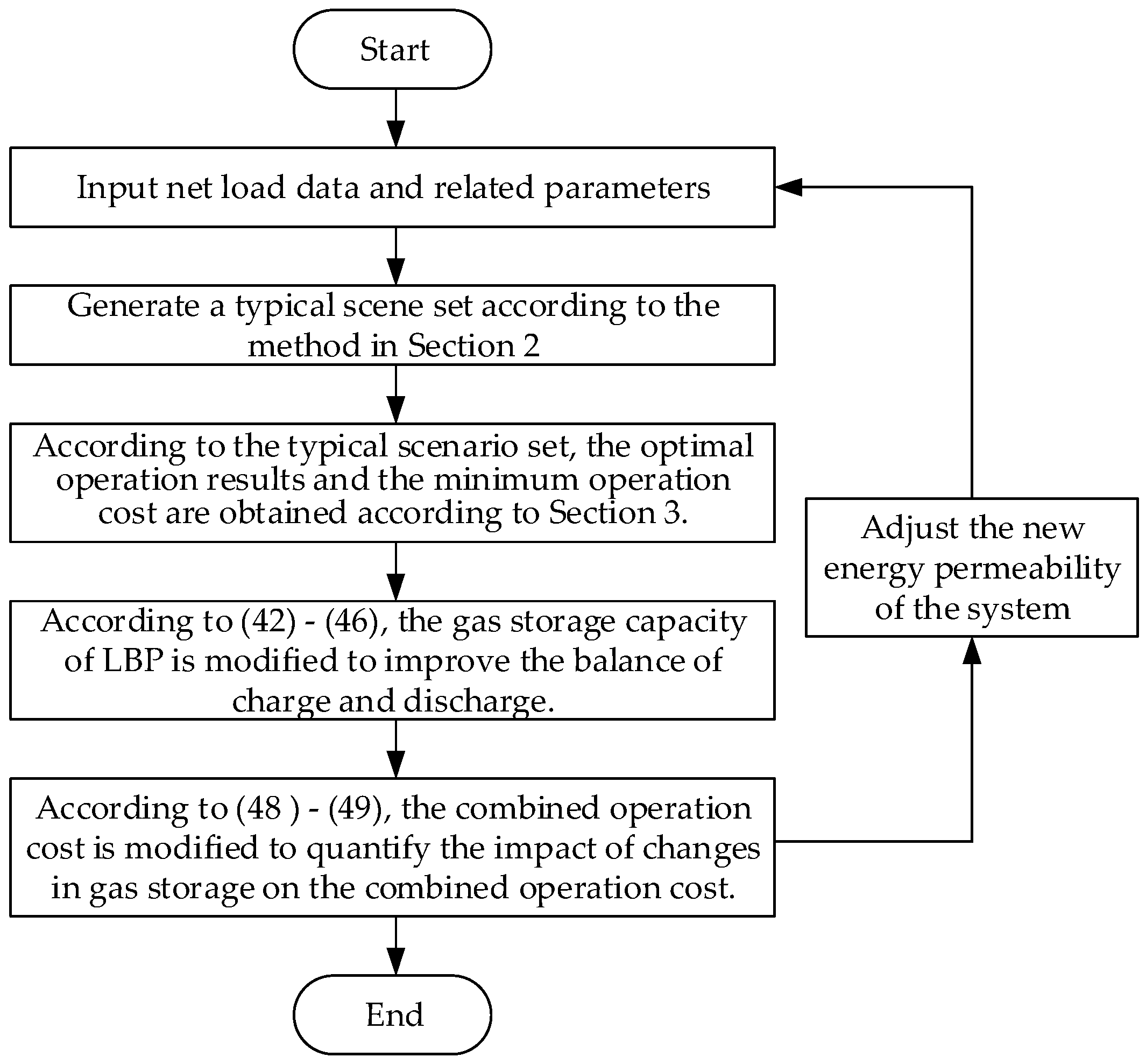
4.3. Capacity Demand Analysis Flow

In summary, the flow chart of capacity demand analysis of rural biogas power generation system with independent operation considering source-load uncertainty is shown in Figure 2.

The optimization problem addressed in this paper is formulated as Mixed Integer Linear Programming (MILP), for which CPLEX serves as a commercial solver capable of efficiently tackling large-scale instances. Utilizing the CPLEX solver, the model presented in this paper is solved to attain optimal solutions.

5. Case Study

5.1. Case Data Sources and Parameters

The conventional power supply consists mainly of thermal power units with an installed capacity of 5720 MW; the total installed capacity of wind turbines is 2356 MW, and the total installed capacity of photovoltaic power generation is 2307 MW. When using the QRA method, the quantiles are set to 0, 0.05, …, 0.95, and 1, and the number of typical scenarios is set to 10. The weight values of the two targets are set to 0.5 for correcting the installed capacity of biogas-generating units.

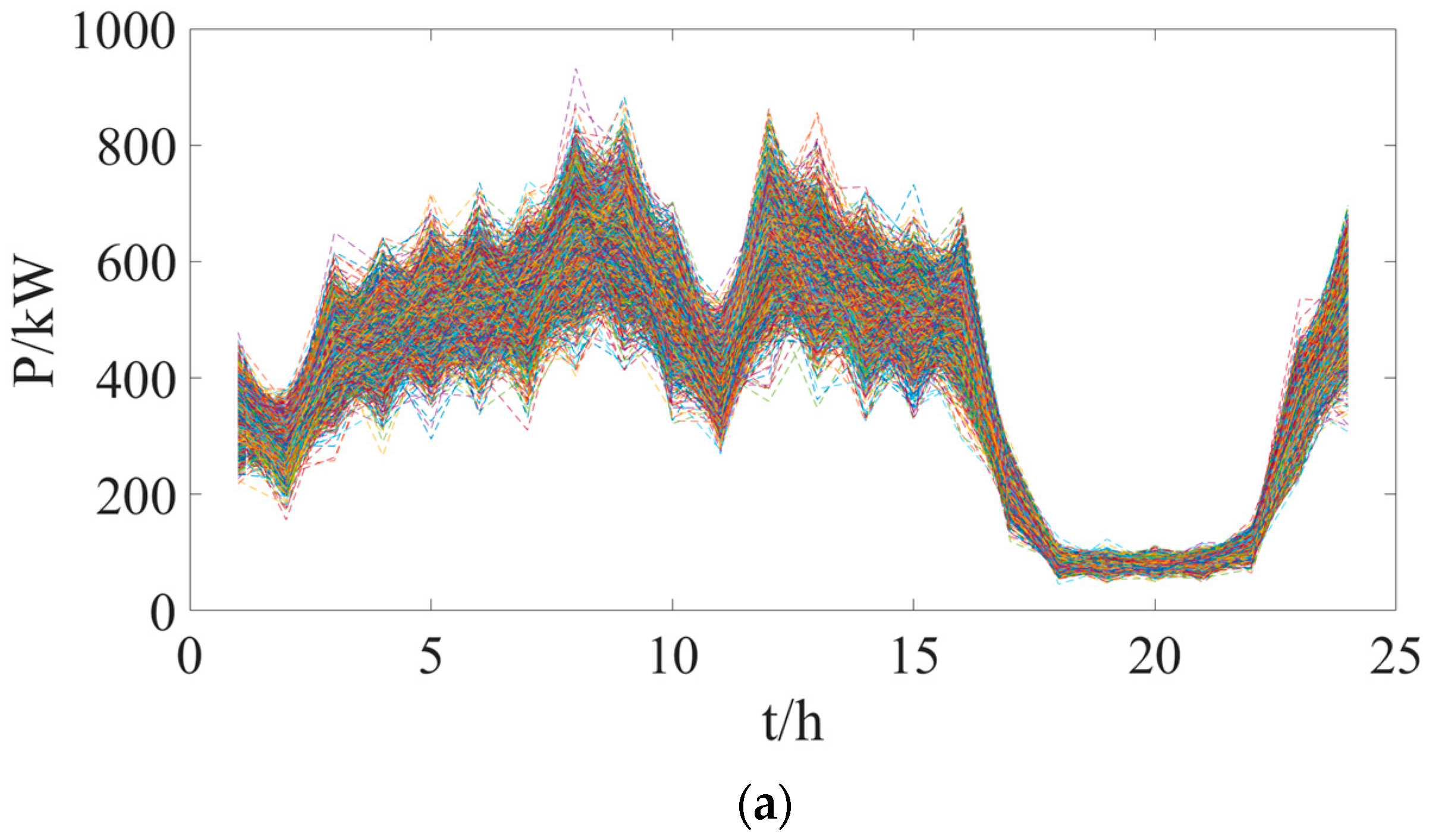
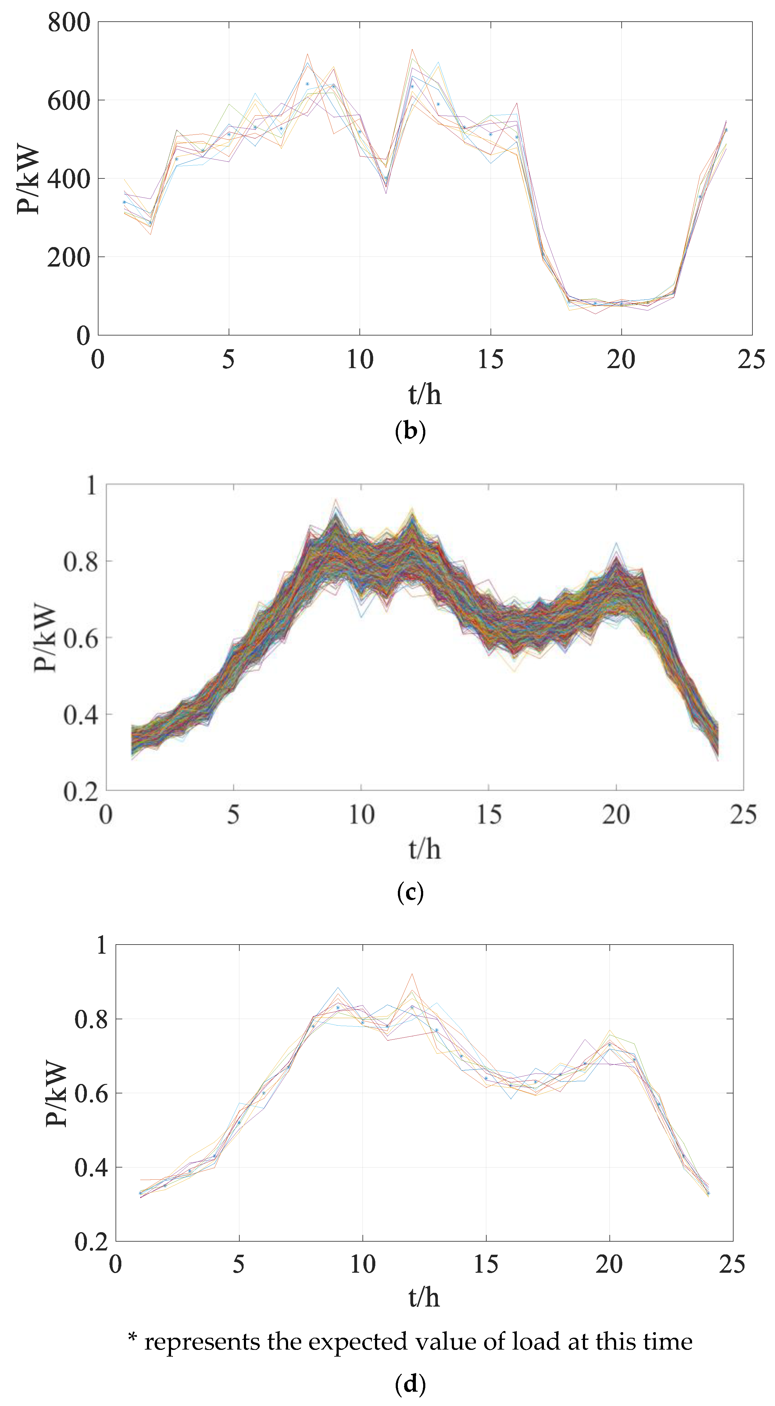
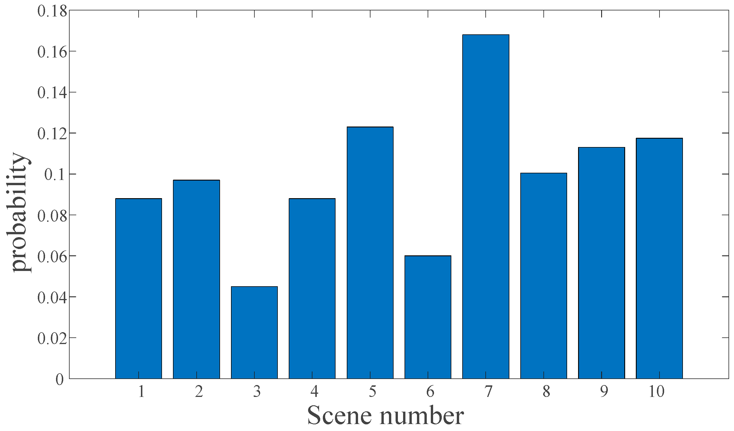
5.2. Typical Scene Set Generation Results

Based on the regional power grid data described in Section 3, the method and calculation process in Section 2.3 is used to generate a typical scene set. The generated typical scene set and its probability are shown in Figure 3 and Figure 4.

5.3. Determination of Energy Storage Demand Capacity

Taking a farm as an example,

Table 1. Generate related parameters of S₀.

	1	2	3	4	Total
Quantity	1418	54	4020	6030	11,526
S0	13,187.4	477.9	7336.5	27,044.55	48,046.35

counts the S₀ of four kinds of animals.

Although the joint optimization operation results have made the operating cost the smallest, because the model does not consider the capacity limit of energy storage, the charging/discharging capacity of energy storage produces a significant imbalance, which generates a large demand for gas storage capacity and increases the cost of gas storage construction. The energy storage power needs to be corrected according to Section 4.2 to avoid this situation. System operation cost before and after energy storage power correction is shown in

Table 2. System operation cost before and after energy storage power correction.

Scene Number	System Operation Cost		The Amount of Cost Increase after Correction
	Before Correction	After Correction
1	1751.08	1774.26	23.18
2	1696.89	1707.26	10.37
3	1988.57	2007.41	18.84
4	1842.75	1869.02	26.27
5	2159.71	2183.64	23.93
6	2010.05	2022.43	12.38
7	1667.02	1681.78	14.73
8	1996.57	2037.85	41.28
9	1687.91	1713.44	25.53
10	2111.80	2124.36	12.56

.

The revised cost increase is not apparent, the maximum increase rate is only 2.02% of the typical day 3, and the minimum increase rate is 2.06% of scenario 8, indicating that the capacity correction method of biogas power generation system proposed in this paper can reduce the imbalance degree of gas charging/discharging with a small operating cost growth rate.

6. Conclusions and Foresight

6.1. Conclusions

This paper proposes a method for determining the demand capacity of a biogas power generation system for the new energy, high-permeability system from the system point of view. The main conclusions are as follows.

(1)

A method is proposed to describe the uncertainty of the pure load demand of a high permeability system of new energy. In the traditional power system dispatching operation method, the calculation is only carried out through a single new energy and load forecasting, which greatly increases the impact of source-load uncertainty. In the method proposed in this paper, on the premise of obtaining typical scenarios, the probability of each scenario can also be calculated, which reduces the impact of pure load demand uncertainty on system scheduling operation.

(2)

The GAD and CGR indexes are introduced to address both the utilization rate of energy storage and operating costs. Subsequently, a modified model integrating these indexes is formulated to determine the demand capacity. The example results demonstrate that the proposed model substantially mitigates gas storage construction costs and charging/discharging imbalances, with a maximum increase in system operating costs of only 2.07%.

6.2. Foresight

(1)

The results of this paper can provide some theoretical guidance for the energy storage configuration in the future new energy, high-permeability system, but the relationship between the new energy consumption level and the energy storage capacity demand is not studied, and the related research work will be carried out in the future.

(2)

In this paper, only the number of scenes is reduced to 10, without demonstrating whether it is reasonable to choose 10 typical scenes. In the follow-up study, the number of scenes should be reduced as much as possible under the premise of ensuring the calculation accuracy. The research on clustering error can be carried out to make the selection of the number of typical scenes more reasonable.

References

1. Xu, G.; Cheng, H.; Ma, Z.; Fan, S. Overview of ESS planning methods for alleviating peak-shaving pressure of grid. Electr. Power Autom. Equip. 2017, 37, 3–11. [Google Scholar]
2. Frazier, A.W.; Cole, W.; Denholm, P.; Greer, D.; Gagnon, P. Assessing the potential of battery storage as a peaking capacity resource in the United States. Appl. Energy 2020, 275, 115385. [Google Scholar] [CrossRef]
3. Li, J.; Yue, P.; Li, C.; Zhang, Z.; Wang, R. Control strategy of energy storage system in wind farm group to improve wind energy utilization level. Electr. Power Autom. Equip. 2021, 41, 162–169. [Google Scholar]
4. Zhu, Y.; Qin, L.; Yan, Q.; Zhang, X. Wind-storage combined frequency regulation strategy and optimal configuration method of energy storage system considering process of frequency response. Electr. Power Autom. Equip. 2021, 41, 28–35. [Google Scholar]
5. Chen, H.; Liu, C.; Xu, Y.; Yue, F.; Liu, W.; Yu, Z.H. The strategic position and role of energy storage under the goal of carbon peak and carbon neutrality. Energy Storage Sci. Technol. 2021, 10, 1477–1485. [Google Scholar]
6. Sun, W.; Pei, L.; Xiang, W.; Sang, B.; Li, G.; Xi, P. Evaluation method of system value for energy storage in power system. Autom. Electr. Power Syst. 2019, 43, 47–55. [Google Scholar]
7. Huang, H.; Zhou, M.; Zhang, L.; Li, G.; Sun, Y. Joint generation and reserve scheduling of wind-solar-pumped storage power systems under multiple uncertainties. Int. Trans. Electr. Energy Syst. 2019, 29, e12003. [Google Scholar] [CrossRef]
8. Zhang, B.; Sun, Y.; Zhang, S. Second-order cone programming based probabilistic optimal energy flow of day-ahead dispatch for integrated energy system. Autom. Electr. Power Syst. 2019, 43, 25–33. [Google Scholar]
9. Xu, C.; Xu, X.; Yan, Z.; Li, H. Distributionally robust optimal dispatch method considering mining of wind power statistical characteristics. Autom. Electr. Power Syst. 2022, 46, 33–42. [Google Scholar]
10. Zhang, J.; Cheng, C.; Shen, J.; Li, G.; Li, X.; Zhao, Z. Short-term joint optimal operation method for high proportion renewable energy grid considering wind-solar uncertainty. Proc. CSEE 2020, 40, 5921–5932. [Google Scholar]
11. Luo, E.; Zhang, Y.; Feng, Y.; Zhu, L.Z. The research on cours, current situation and future direction of China’s biogas industry development-Based on the typical case analysis of Luohe area, Henan. Chin. J. Agric. Resour. Reg. Plan. 2022, 43, 132–142. [Google Scholar]
12. Li, J.; Li, B.; Xu, W. Analysis of the policy impact on China’s biogas industry development. China Biogas 2018, 36, 3–10. [Google Scholar]
13. Wang, Z.Q.; Wang, J.; Ma, M.I.; Yang, H.; Chen, D.; Wang, L.; Li, P. Distributed event-triggered fixed-time fault-tolerant secondary control of islanded AC microgrid. J. IEEE Trans. Power Syst. 2022, 37, 4078–4093. [Google Scholar] [CrossRef]
14. Xu, D.; Zhou, B.; Chan, K.W.; Li, C.; Wu, Q.; Chen, B.; Xia, S. Distributed multienergy coordination of multimicrogrids with bio-gas-solar-wind renewables. IEEE Trans. Ind. Inform. 2019, 15, 3254–3266. [Google Scholar] [CrossRef]
15. Zhou, B.; Xu, D.; Li, C.B.; Chung, C.Y.; Cao, Y.; Chan, K.W.; Wu, Q. Optimal scheduling of biogas-solar-wind renewable portfolio for multicarrier energy supplies. IEEE Trans. Power Syst. 2018, 33, 6229–6239. [Google Scholar] [CrossRef]
16. Ghaem Sigarchian, S.; Paleta, R.; Malmquist, A.; Pina, A. Feasibility study of using a biogas engine as backup in a decentralized hybrid (PV/wind/battery) power generation system-Case study Kenya. Energy 2015, 90, 1830–1841. [Google Scholar] [CrossRef]
17. Yang, H.; Shi, B.; Huang, W.; Samayeh, M. Day-ahead optimized operation of micro energy grid considering integrated demand response. Electr. Power Constr. 2021, 42, 11–19. [Google Scholar]
Figure 1. Biogas power generation flow chart.
Energies 17 01880 g001
Figure 2. The flow chart of capacity demand analysis of rural biogas power generation system with independent operation considering source-load uncertainty.
Energies 17 01880 g002
Figure 3. Typical scene set generation. (a) Before the reduction in new energy output. (b) After the reduction in new energy output. (c) Before load output reduction. (d) After load output reduction.
Energies 17 01880 g003aEnergies 17 01880 g003b
Figure 4. Probability of each typical scene.
Energies 17 01880 g004