Doing More with Less: Applying Low-Frequency Energy Data to Define Thermal Performance of House Units and Energy-Saving Opportunities

Abstract

High-frequency energy data, such as hourly and sub-hourly energy, provide various options for assessing building energy performance. However, the scarcity of such energy data is among the challenges of applying most of the existing energy analysis approaches in large-scale building energy remodeling projects. The purpose of this study is to develop a practical method to define the energy performance of residential house units using monthly energy data that are relatively easy to obtain for existing building stock. In addition, based on the defined energy use characteristics, house units are classified, and energy retrofit measures are proposed for energy-inefficient units. In this study, we applied a change-point regression model to investigate the heterogeneity in the monthly gas consumption of 200 house units sampled from four apartment complexes in Ulsan, Republic of Korea. Using a four-quadrant plane and the fitted model parameters, we identified most energy-inefficient house units and their potential energy-saving measures are assessed. The results indicate that around a 41% energy reduction through enhanced thermal properties and heating systems was achieved. The study responds to the need for a straightforward procedure for identifying and prioritizing the best targets for effective energy upgrades of existing buildings.

1. Introduction

According to the International Energy Agency, buildings alone consume approximately 35% of total energy use and are responsible for over one-third of the CO₂ emitted globally [1]. In most nations, existing building stock has become a prime focus for energy use reduction, as this category makes up the largest part of the building sector. For instance, according to Korean national statistics, as of 2018, only 2% of the existing buildings were newly built or retrofitted to meet the national building energy efficiency regulations [2]. This highlights the need for a more effective approach for achieving sustainability in the building sector.

Various countries have established building remodeling institutions dedicated to the assessment and improvement of buildings in operation. However, it is challenging to define an approach for analyzing aging buildings in terms of energy performance, given that each building has a unique set of features that affect its energy consumption. Juan and Hsing [3] reported that a conventional age for building remodeling depends on the building service under consideration. Their study indicated that the adjustment and improvement of a building’s structure should be carried out 30 years after its completion, while other building features, such as water and sanitary systems, should be inspected and renovated every 15 years. Regarding energy efficiency, defining which buildings (and which parts of a specific building) need to be retrofitted is often a complex task. Variations in the degradation of building energy performance over time (resulting from thermal characteristics and occupant-related factors) invalidate an age-based approach in identifying buildings for energy remodeling. It is necessary to assess the unique energy use of a building to determine its energy efficiency.

Existing buildings are likely to consume more energy than new buildings due to degradation in their energy performance caused by various reasons such as poor or improper maintenance or even natural aging effects [4]. The literature review indicates a wide spectrum of approaches to assess the energy performance of a building, and the applicability of each method is determined by both the scope of analysis and data availability. For instance, a physical-based model approach (such as building energy simulation models) are used to identify the energy performance of a building based on the principles of building interactions with the outdoor environment by convective heat transfer through exterior surfaces and the exchange of air between outside and the indoor conditioned space through infiltration. Although this approach allows a detailed analysis of building energy characteristics, its application is hindered by modeling complexity and a large number of input parameters required to carry out simulations. The alternative approach used to assess the energy consumption of existing buildings is the energy use intensity (EUI) indicator, which is simply the ratio of a building’s energy use to its floor area. Despite EUI being widely used, studies have highlighted that its meaning is less informative in terms of the energy performance of a building, as it relies on the static attributes of a building such as its space use type and floor area rather than its thermal characteristics. For example, a building with a degraded envelope thermal performance can exhibit the same EUI (and hence be classified in the same category) as a high-thermal performance building but with a user-induced high energy consumption. Studies have highlighted the need for an improved method to assess and classify the energy efficiency of existing buildings [5,6].

With recent advancements in computer technology, inverse modeling methods, including artificial intelligence-based approaches, are applied to define energy characteristics of buildings during operation. However, their application is often hindered by the difficulty in obtaining higher frequency energy use data, such as hourly and sub-hourly energy use, particularly for investigations involving large-scale buildings. In the reviewed literature, change-point regression models and other inverse modeling approaches have primarily been used to define a baseline model to benchmark the energy consumption of a building and quantify energy savings from retrofitting measures [7,8]. Afroz et al. [9] compared the capabilities of the change-point regression model and three other inverse models in calculating the energy achieved by the implementation of smart building technology systems in 12 government buildings in Ottawa, Canada. Their study confirmed the flexibility and accuracy of the change-point regression model in providing insights into building energy characteristics with relatively less computational complexity. In addition, some studies have applied change-point regression models to determine outliers in building energy use [10], anomalies in building systems [11], time-based building thermal power characteristics [12], and building energy calibration [13]. Nonetheless, the temporal granularities of energy data (sub-hourly, hourly, or daily) used in these studies are not the most common type of energy data available, especially for residential buildings.

Using monthly utility bills, Park et al. [14] applied change-point regression models in the prediction of thermal performance and energy-saving potentials of apartment complexes. Their study provides a procedure for defining energy characteristics of apartment buildings, which can be used for an estimation of weather-dependent energy demand of residential buildings at a city level. Nevertheless, regressions in their study were developed using data from an apartment complex level rather than data from individual house units. Thus, the interactive effects, as well as occupant energy use behavior of these individual units in an apartment complex, were not considered.

Energy remodeling of existing building stock should involve identifying energy-inefficient buildings, defining retrofitting options and their predicted energy-saving potentials. In recent years, research related to the selection and implementation of energy efficiency measures has increased as various countries focus on energy efficiency in the building sector. From previous studies, several energy-saving measures have been proposed, ranging from low cost and passive strategies [15] such as energy-efficient equipment and the advanced operation and control of building systems, to more advanced options such as smart retrofitting measures [16] (e.g., the installation of smart sensors and automation control and management). A study by Hart et al. [17] reported that a 7–16% reduction in energy demand could be achieved by upgrading the window glazing of residential buildings in different climate zones in the United States, while a 15% energy reduction was estimated by retrofitting windows of a residential building in Brazil [18]. Gugul et al. [19] indicated that improving the building envelope of a single-family house under Turkey’s climate could result in a 50% reduction in heating energy demand. In the case of Republic of Korea, Seo et al. [20] investigated the energy reduction of green retrofitting energy-inefficient apartment complexes that were defined based on building age. The study reported that around a 32% heating energy reduction can be achieved by improving window U-values and SHGC and infiltration rates.

The literature review on the energy retrofitting of existing building stock reveals that studies addressing the key point of identifying targeted buildings for energy retrofitting are lacking. The majority of previous studies have investigated energy retrofitting for selected buildings based on their energy consumption assessed using the EUI indicator or building age [20]. Building energy consumption is influenced by multiple factors, hence an accurate diagnosis of energy use characteristics and the identification of the most energy-inefficient buildings should precede the (identification) assessment of effective energy retrofit measures for existing building stock. A more systematic approach is needed to categorize high-energy-consuming buildings as a result of poor thermal performance rather than operation-related factors.

The purpose of this study was to develop a practical method to classify the energy characteristics of residential houses and identify potential targets for energy remodeling. We assessed the dependency of heating energy use on the outdoor temperature for house units from apartment complexes through a change-point regression model and monthly utility billing records. We categorized house units based on their energy use characteristics, and we identified high-energy-consuming houses (due to building thermal performance or occupant-related factors). We explored energy retrofit options and quantified their energy-saving potentials. Our study responds to the need for a straightforward procedure to define building energy characteristics and to prioritize existing buildings for energy retrofits using data that are relatively easy to obtain. For large-scale building energy retrofit projects (such as green remodeling in Republic of Korea), a key challenge is identifying buildings with low energy performance and potential energy-saving options in a reliable and cost-effective manner. The findings of this study may serve as a foundation for developing guidelines for the energy remodeling of existing building stock at a regional or national level.

2. Methodology

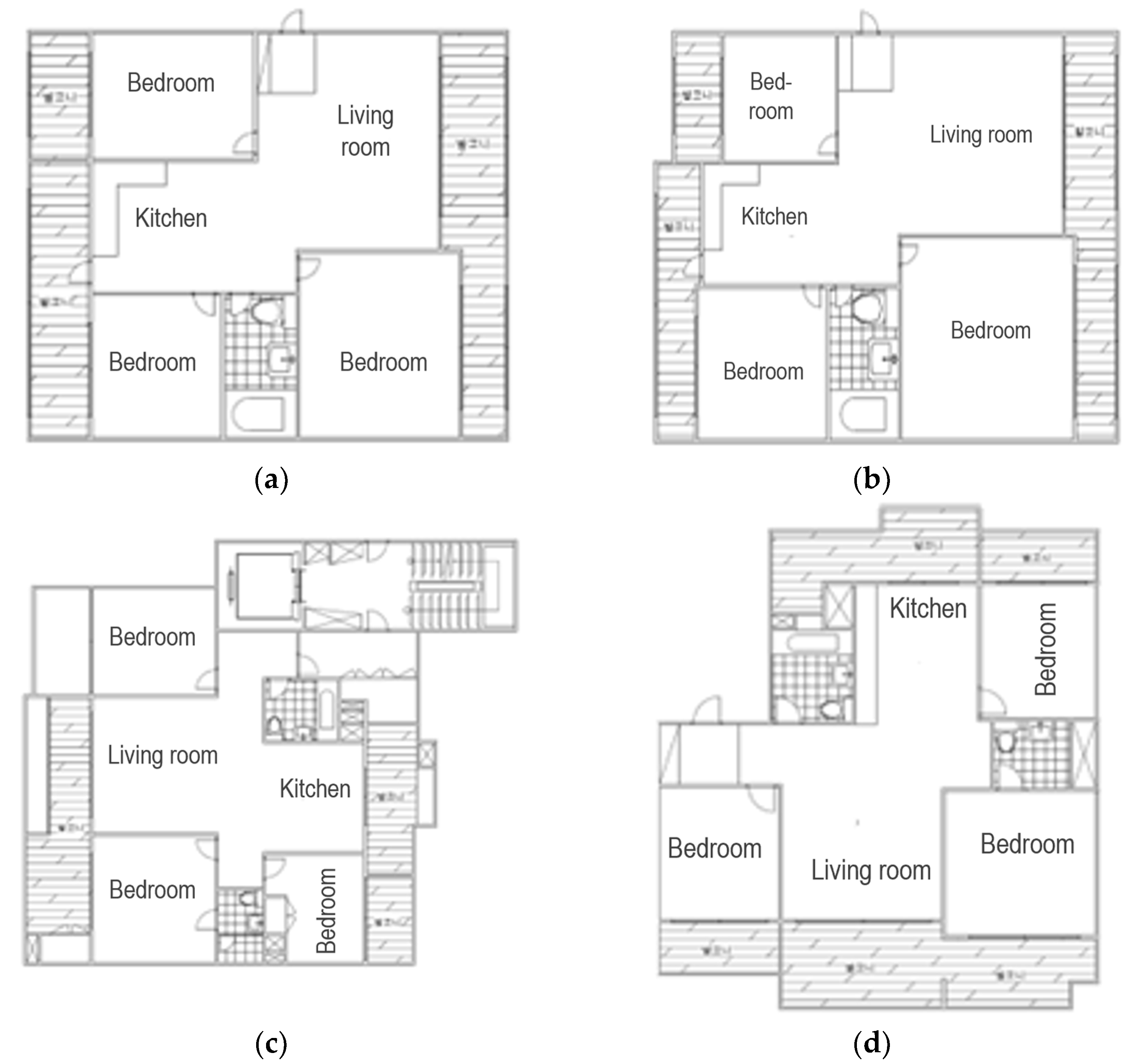
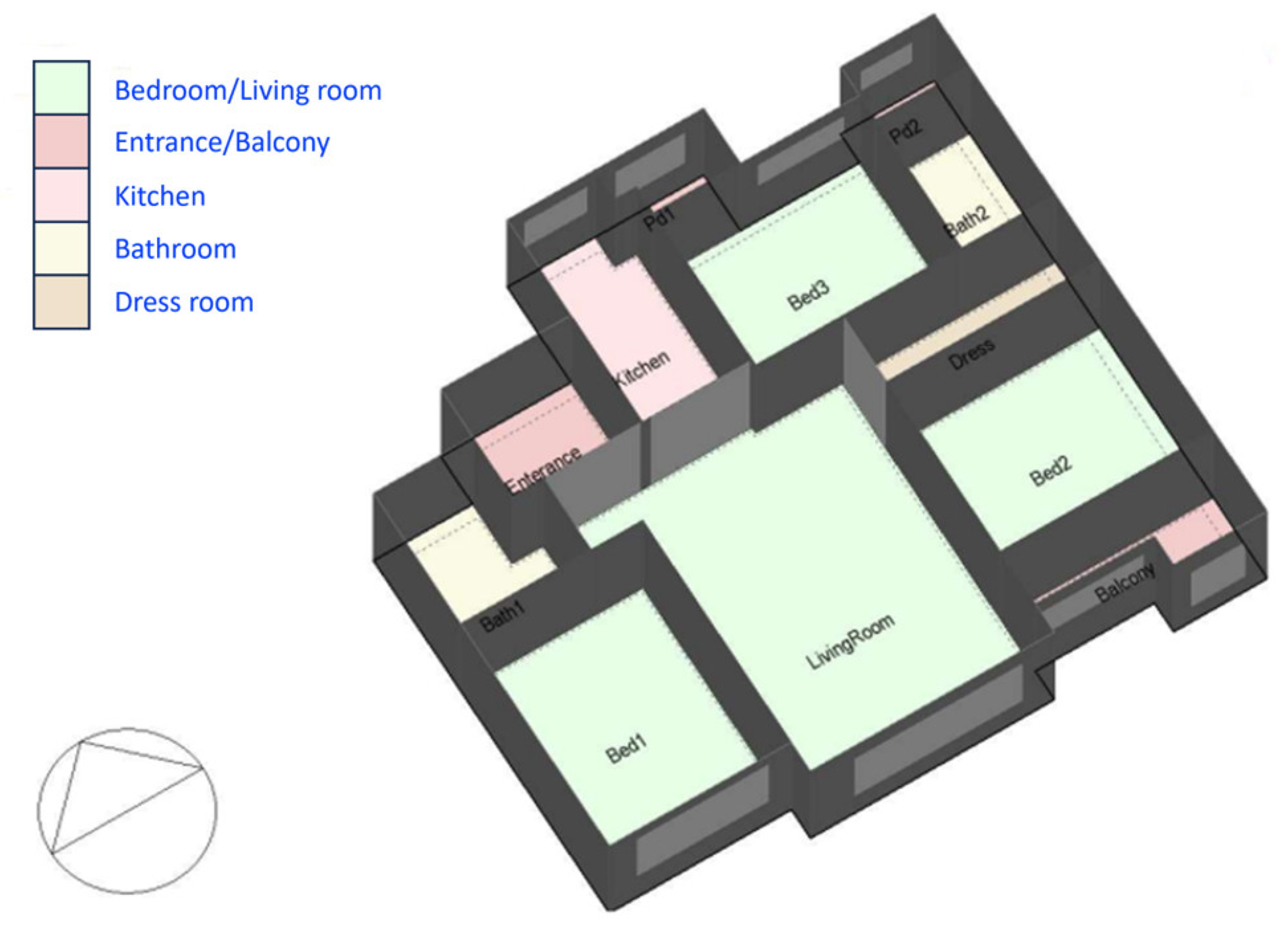
2.1. Overview of the Sample

This study characterizes the energy use of house units from existing apartment complexes in Ulsan, Republic of Korea. The study’s sample was selected to represent aging apartment complexes in the city. Apartment complexes in Ulsan are classified into flat plate apartments and tower apartments. Given that most of the apartment complexes designed and constructed before the year 2000 are the flat type, only flat plate apartments were selected for this study. In addition, only apartment complexes with more than 300 house units and with individual heating systems using natural gas for floor heating were selected.

We sampled four apartments: A, B, C, and D, built in 1991, 1996, 2001, and 2006, respectively. They are multi-family residential buildings containing several single-household units on each floor. The external walls of these apartments are built of reinforced concrete, while walls between adjacent house units are filled with concrete. To ensure consistency in the data, we selected individual house units in each complex based on the floor area, the floor level, and the unit’s position relative to adjacent house units. For each complex, house units were evenly selected from the low, middle, and top floors, and also from side-located and middle-located house units, as illustrated in

Table 1. House unit (HU) characteristics from the four sampled apartment complexes.

Apartment	Year of Completion	Floor Area (m2)	HU Location	HU Floor Level			HU
				Low (Ratio)	Middle (Ratio)	Top (Ratio)
A	1991	86.41	Side	4 (8%)	5 (10%)	3 (6%)	50
			Middle	9 (18%)	16 (32%)	13 (26%)
B	1996	84.28	Side	4 (8%)	4 (8%)	2 (4%)	50
			Middle	14 (28%)	16 (32%)	10 (20%)
C	2001	106.32	Side	5 (10%)	4 (8%)	4 (8%)	50
			Middle	16 (32%)	8 (16%)	12 (24%)
D	2006	87.26	Side	4 (8%)	5 (10%)	6 (12%)	50
			Middle	14 (28%)	10 (20%)	11 (22%)

. In addition, to control the effect of orientation on building energy consumption, only south-facing units were selected. This study’s sample included 200 house units (50 individual house units from each apartment complex). The share of house units from the low, middle, and top floors in the sample was 35%, 34%, and 31%, respectively. The percentage of house units located at the side of the apartment building was 25% of the sample. The floor area of the house units ranges from 84.28 to 106.32 m², and all house units have three bedrooms (located in the corners) and a living room at the center. Figure 1 shows floor plans of the house units from the selected apartment complexes.

2.2. Data

In inverse modeling, the quality of the dataset plays a crucial role in the accuracy of the developed model. The ideal approach is to use a dataset with enough energy consumption data covering the full energy behavior of a building. In the sampled apartment complexes, natural gas is supplied to individual house units for space heating, cooking, and domestic hot water. For the purpose of this study, monthly gas consumption data for the selected 200 house units were collected for a period of one year (from December 2010 to November 2011). Gas consumptions of sampled apartment complexes were retrieved from the Korea City Gas Association website [21], which is a nationwide platform developed to provide data on natural gas use in residential buildings. In Korea, apartments are equipped with gas meters to record the gas consumption of each individual house unit. The readings on the gas meter are recorded by the city gas company and monthly bills are issued to residents based on static pricing that defines the price per m³ of gas. For convenience, gas consumption units on the utility bills were converted from m³ to kWh. In addition, it is important to normalize the energy consumption of each house unit to its floor area (kWh/m²) to enable accurate comparisons between individual house units. Non-heated spaces such as balconies and bathrooms were not included in the floor areas used for energy normalization.

Inverse models use local weather data for fitting model parameters of a building. We used the weather data of Ulsan, Republic of Korea (obtained from Ulsan metropolitan weather station), to develop a regression model for each individual house unit. We used the hourly outdoor temperatures of the weather recordings from December 2010 to November 2011 to calculate monthly average temperatures.

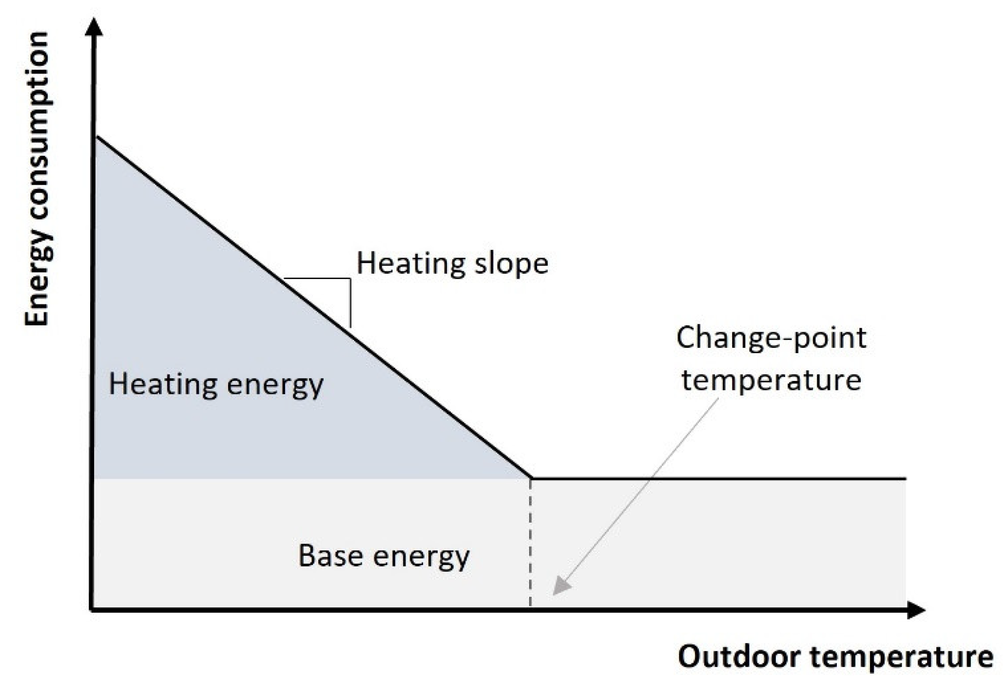
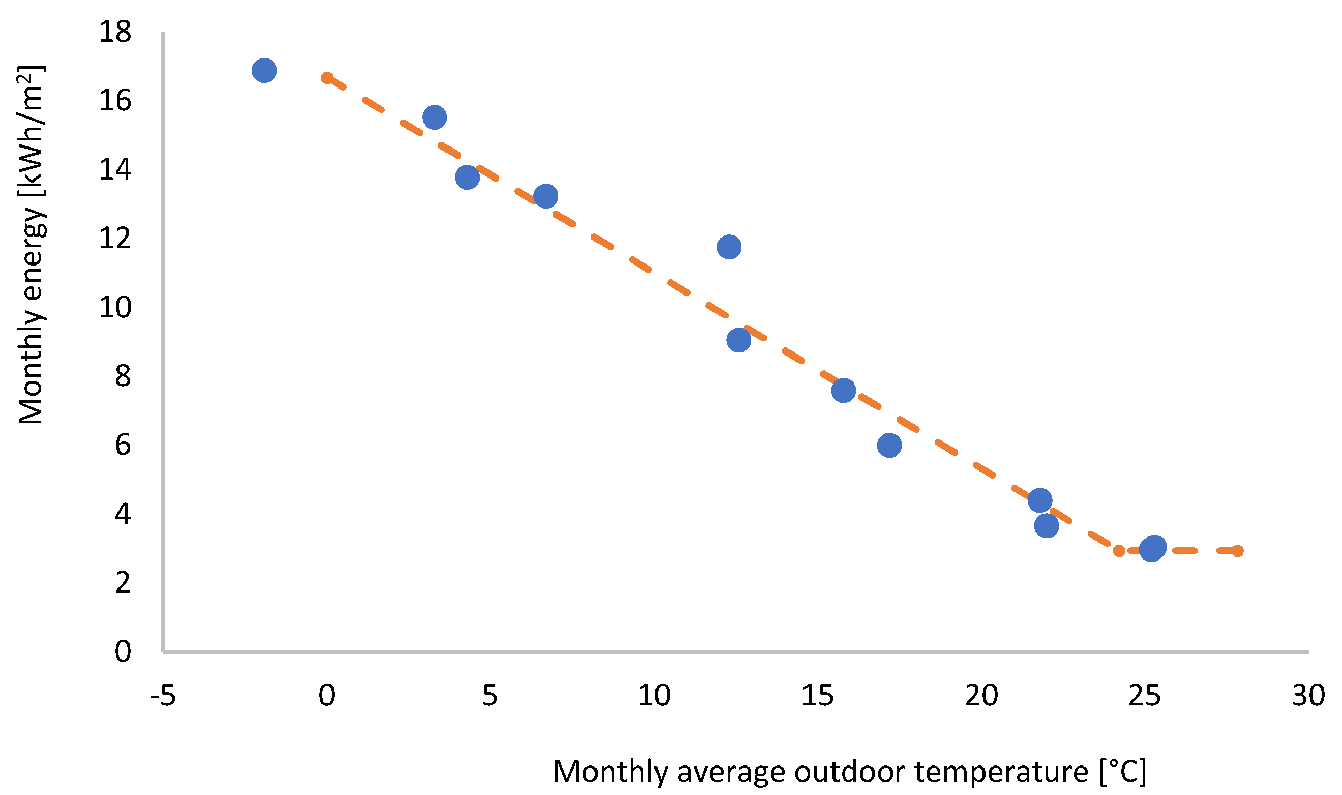
2.3. Model Development

The change-point regression model is among the most used inverse models for characterizing a building’s energy use as a function of outdoor air temperature. The model’s algorithm, developed by Kissock et al. [22], uses piece-wise linear regression equations to find change-point temperature at which building energy consumption switches between seasonal trends. One of the advantages of change-point regression models is their ability to provide sufficiently accurate characterization of building energy consumption with less computational cost and data requirements [23]. The two main inputs of the models are energy use data and the corresponding weather data. Generally, for the independent variable of change-point regression models, the ambient temperature is the most commonly used, given that the outdoor temperature is more statistically influential to the energy consumption of buildings in comparison to other weather parameters such as relative humidity, wind speed, etc. [10,24]. A study by Do and Cetin [25] has reported the applicability of change-point models in different climate zones. The first step in change-point regression modeling is the selection of a statistical parameter model that best describes the characteristics of the energy consumption of the building under consideration. ASHRAE (American Society of Heating, Refrigerating and Air-Conditioning Engineers) [22] describes five change-point regression models and their applications based on different building energy systems.

In this study, a three-parameter change-point regression model was selected to describe natural the gas consumption of each house unit. As shown in Figure 2, the model parameters are as follows: heating slope ($S_h$); heating change-point temperature ($T_{cph}$); and base energy ($E_{base}$). The heating slope indicates the linear dependency of gas consumption on outdoor temperature below a certain temperature. This parameter is used to calculate weather-dependent energy use, which, in this case, is the space heating energy used by the sampled house units. The model also defines heating change-point temperature (above which no space heating is needed in the house unit) and a base energy (the non-weather-dependent energy used for activities such as cooking and domestic hot water). The monthly natural gas consumption, $E$, can be defined as a function of $E_{base}$, $S_h$, $T_{cph}$, and outdoor temperature ($T_{oa}$) as shown in Equation (1). After determining the model parameters, we calculated the space heating energy ($E_h$) for each house unit using Equation (2).

$$E=E_{base}+S_h(T_{cph}-T_{oa}){}^{+}$$

(1)

$$E_h=S_h\left(T_{cph}-T_{oa}\right){}^{+}$$

(2)

where $E$ is the monthly energy consumption, $E_{base}$ is the monthly base energy consumption, $S_h$ is the heating slope, $T_{cph}$ is the heating change-point temperature, $T_{oa}$ is the average monthly outdoor temperature, and $E_h$ is the heating energy consumption. The superscript in Equations (1) and (2) indicates that the value in parentheses is zero for negative values.

In change-point regression modeling, parameters are defined by the best fit regression line that minimizes the sum of the squares of the difference between the actual energy consumption and that predicted by the regression equation. One drawback of the change-point regression model is that it is not applicable to buildings with inconsistent energy consumption. According to ASHRAE guidelines [26], a model is considered fit to characterize the energy use of a given building if the resulting regression’s goodness of fit, R², is above 0.75 and its CV (RMSE) (coefficient of variation of the root mean squared) is below 0.15 for monthly energy consumption. Therefore, in this study, we selected house units that meet the R² and CV (RMSE) guidelines.

3. Results

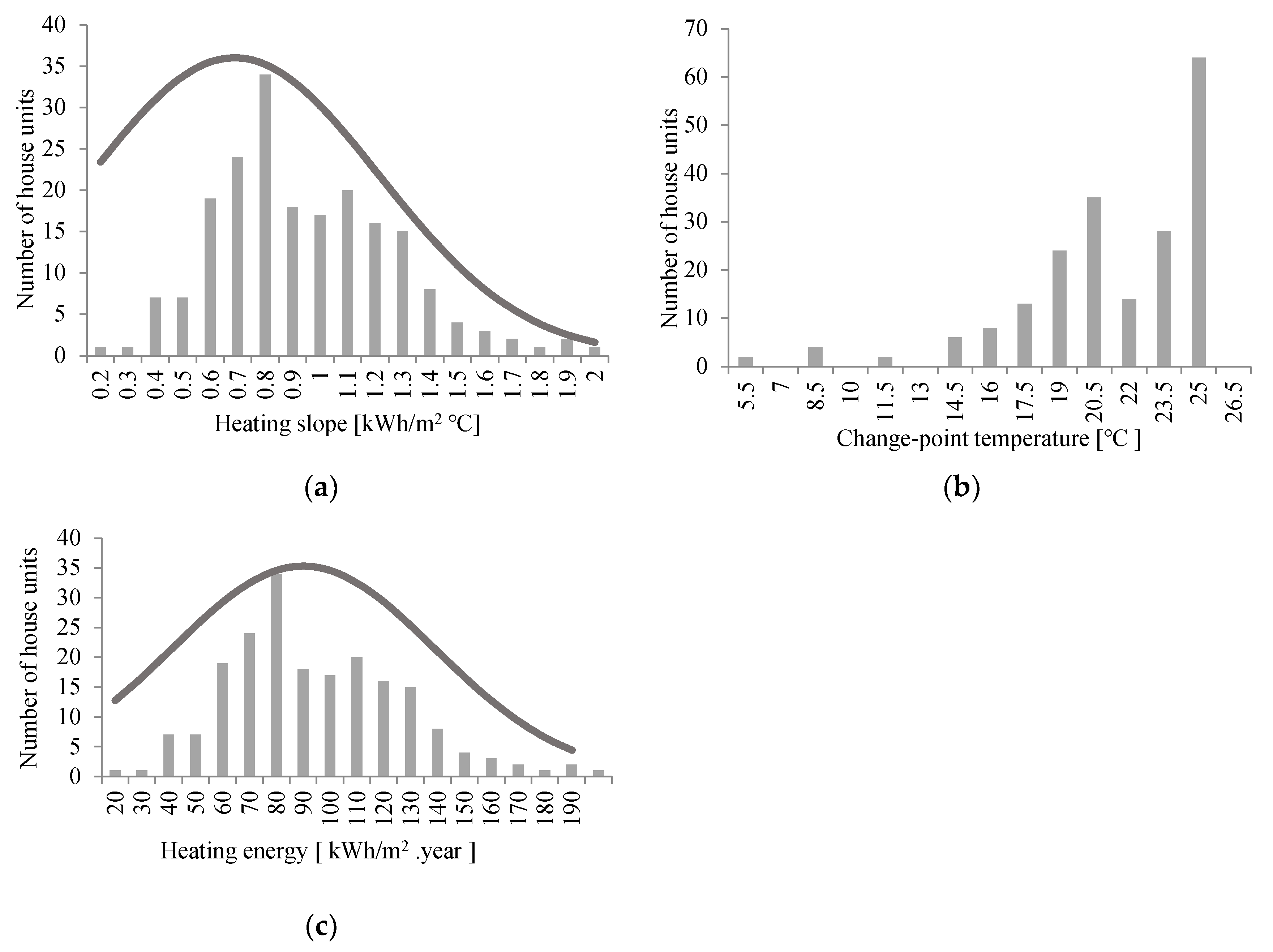
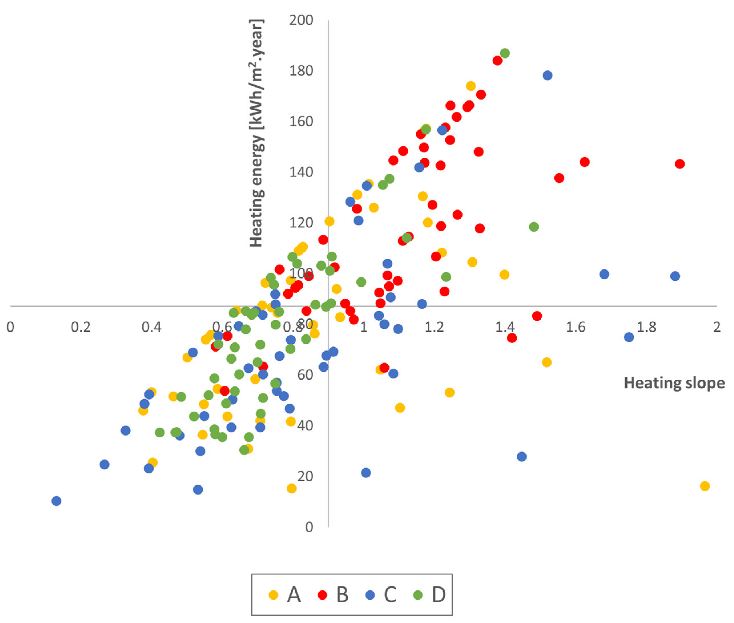
3.1. Change-Point Regression Model Results

Figure 3 illustrates monthly energy use from a sampled house unit as a function of monthly outdoor temperature. The figure shows the actual energy consumption (represented by the blue dots) and the predicted energy use (indicated by the dashed line). For all the sampled house units, R² is above 0.75, and the CV (RMSE) is below 0.15. For detailed regression results for each sampled house unit, refer to the Supplementary Materials of this study. The study’s results from the change-point regression model indicate that the three-parameter model is able to characterize the gas consumption of house units in the sampled apartment complexes.

Figure 4a shows the distribution of the obtained change-point regression parameters for all the sampled house units. The heating slope, $S_h$, which indicates the impact of decreasing outdoor temperatures on the amount of energy used for space heating, varies between house units and ranges from 0.21 to 2.01 kWh/m² °C, with an average of 0.89 kWh/m² °C. The variation in $S_h$ is linked to the thermal characteristics and heating system efficiency of the building. As expected, around 62% of the house units with a low heating slope are from the younger apartment complex D, which was built in compliance with revised standards for building insulation.

Figure 4b illustrates the results for the heating change-point temperature $T_{cph}$ of the sampled house units, which ranges from 5.5 °C to 25.4 °C, with an average value of 20.5 °C. Unlike the heating slope, variations in the obtained heating change-point do not show any particular trend between the house units of the four apartment complexes under consideration. This is due to the high variability in user behavior within residential buildings. Our results indicate that the change-point temperature parameter is more closely linked to factors related to occupants (such as the heating setpoint temperature) than to the overall energy performance of a building.

Figure 4c shows the heating energy use calculated using Equation (2). The results indicate that the energy used for space heating in the sampled house units ranged from 20.4 to 190.2 kWh/m² per year, with an average of 87.1 kWh/m² per year. Variation in the heating energy use is due to differences in building performance and operation. While heating energy use of a building is a key aspect of the building energy assessment, this information alone cannot reveal all the unique characteristics of a building and is not sufficient to determine the building’s energy-saving potential.

The variations in the change-point regression model parameters of house units from each apartment complex are shown in

Table 2. Results from change-point regression model by apartment complex.

Apart. (Year)	Model Parameters
	${\mathit{S}}_{\mathit{h}}$ [kWh/m2·C]	${\mathit{T}}_{\mathit{c}\mathit{p}\mathit{h}}$ [°C]	${\mathit{E}}_{\mathit{h}}$ [kWh/m2·Year]
A (1991)	0.87 ± 0.31	20.69 ± 4.68	83.6 ± 37.1
B (1996)	1.11 ± 0.26	21.60 ± 2.53	116.4 ± 33.0
C (2001)	0.84 ± 0.37	19.36 ± 4.16	70.3 ± 35.9
D (2006)	0.77 ± 0.23	21.05 ± 2.79	82.9 ± 33.1

. Note that the overall energy use characteristics of the house units do not reflect the common assumption that older buildings are the most energy-inefficient and should be prioritized for energy remodeling. For instance, while the heating energy consumption in apartment A (1991) is relatively similar to that of apartment D (2006), the average heating energy use in apartment C (2001) is 60.1% of the amount used by apartment B (1996), which consumed the highest heating highest energy. These results indicate that an age-based energy retrofitting approach would not be an effective way to improve the energy performance of existing building stock. In addition, the high variability in energy use characteristics of house units in the same apartment complex highlights the need for house unit-level energy assessments rather than the overall performance of a building in its entirety. This is particularly true for multi-residential buildings in which the energy use is greatly influenced by occupant-related factors.

3.2. Energy-Inefficient House Units

Generally, a high energy consumption value for a building can be due to its low energy performance or due to occupant-related factors. While the former can be addressed by measures such as energy remodeling, the latter can be addressed by simply encouraging efficient energy-use behavior. Therefore, to assess energy-saving potentials of a given building, particularly a residential building, the first step should be to understand its energy consumption.

In this study, to identify the specific energy use characteristics of each house unit, we used a plane with four quadrants. The plane’s origin represents the average heating slope and heating energy from the sampled house units (Figure 5). In this way, house units are classified into four categories representing their energy use features.

House units in the first quadrant (upper right quadrant) have a high heating slope (sensitivity to outdoor temperature variation) and a high heating energy consumption. This implies that the energy performance of these houses can be enhanced by improving the thermal performance of the external envelope and the efficiency of the heating equipment. In the second quadrant (low heating slope and high heating energy consumption), the house units are characterized by high user-induced energy consumption. This category may include house units occupied by people with particular indoor thermal requirements (such as children, elderly occupants, or simply occupants with special preferences in terms of indoor conditions). The third quadrant (lower left quadrant) consists of house units with a low heating slope and a low heating energy consumption. A low heating slope indicates a low sensitivity of heating energy to outdoor temperature variations as a result of good building thermal performance. Therefore, house units in the third quadrant are classified as energy efficient house units. The last category, the fourth quadrant, has house units characterized by a high heating slope (poor thermal performance) but low heating energy use (due to occupant schedules or the intermittent operation of heating systems).

Table 3. Number of house units in each quadrant, according to apartment complex.

Apart. (Year)	Quadrant
	First	Second	Third	Fourth
A (1991)	15 (21.1%)	10 (43.5%)	10 (13.0%)	15 (51.7%)
B (1996)	34 (47.9%)	5 (21.7%)	5 (6.5%)	6 (20.7%)
C (2001)	11 (15.5%)	8 (34.8%)	29 (37.7%)	2 (6.9%)
D (2006)	11 (15.5%)	0 (0%)	33 (42.9%)	6 (20.7%)
Total	71 (100%)	23 (100%)	77 (100%)	29 (100%)

indicates the number of house units in each quadrant and the percentage of house units from each apartment complex. As shown in the table, approximately 70% of house units identified as energy inefficient (first quadrant) are from the older apartment complexes A and B, while more than 80% of the most energy-efficient house units (third quadrant) are from the younger apartment complexes C and D. These results show that revisions in building standards over the years have positively impacted the overall energy consumption of apartment complexes, although the amount of this impact varies.

3.3. Energy-Saving Potential

As indicated in the previous section, the majority of house units defined as energy-inefficient (first quadrant) were in apartment complex B. Therefore, in our study, we made use of a house unit in apartment B for the study’s base model, and we assessed its energy consumption using DesignBuilder v7/EnergyPlus v9.4 simulation tools. The ability of DesignBuilder/EnergyPlus to accurately predict energy consumption of a building has been well documented [27].

The base model consisted of five conditioned zones: three bedrooms, a living room, and a kitchen (Figure 6). Building characteristics, such as orientation, window-to-wall ratio, total and heated floor area, etc., were collected through site visits and internet searches. Regarding the model’s thermal properties, we used Korean building regulations from the year 1996 (when apartment complex B was built) to define the model’s envelope elements.

Table 4. Base model description as designed in DesignBuilder/EnergyPlus.

Input Parameter		Value
Physical aspect	Floor area	84.99 m2
	Height	2.80 m
	Window-to-wall ratio	25.15%
	Orientation	South
Thermal property	Wall U-value	0.72 W/m2 K
	Window U-value	3.48 W/m2 K
	Roof U-value	0.58 W/m2 K
	Infiltration rate	3.71 ACH50
System & operation	System	Radiant floor heating
	Boiler efficiency	0.70
	Lighting	8.5 W/m2
	Occupancy	0.03 people/m2
	Heating setpoint	21 °C

shows the characteristics and input parameters of the model designed in the DesignBuilder/EnergyPlus program. In addition, an EPW (EnergyPlus weather data) file for 12 months (December 2010 to November 2011) was created and used in the simulation. The predicted heating energy was compared with the actual gas consumption of the housing unit for model validation (see Section 3.3.1).

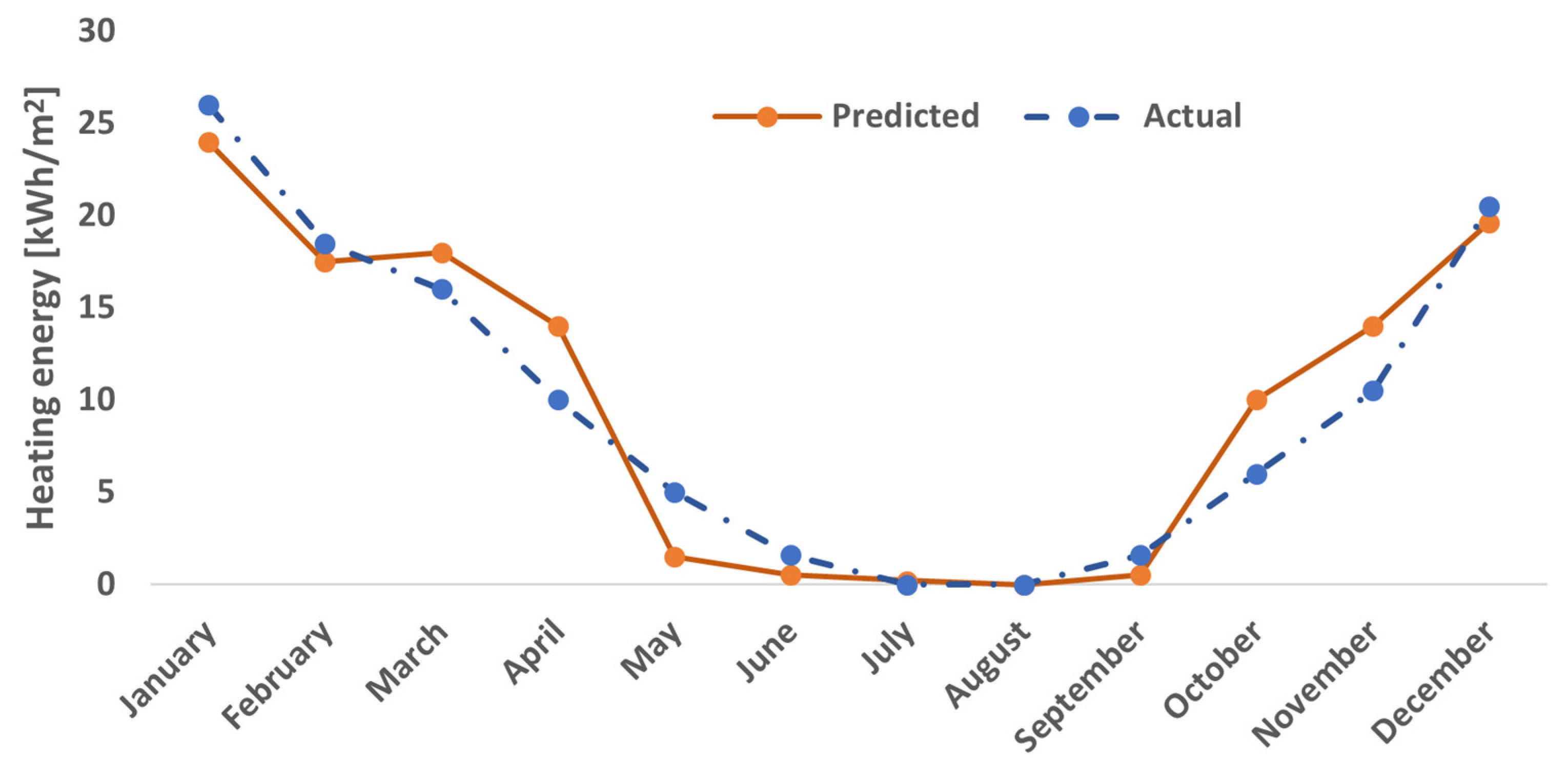
3.3.1. Model Validation

With energy simulation, it is important to calibrate the model so that its energy prediction matches the actual energy use of the building under consideration. ASHRAE Guideline 14-2014 [28] recommends three indicators for model validation, and among them, the CV (RMSE) is used in this study. The CV (RMSE) is calculated as shown in Equation (3). According to ASHRAE, its value should be less than 15% for monthly energy.

$$CV\left(RMSE\right)={\displaystyle \frac{1}{\overline{m}}}\sqrt{{\displaystyle \frac{{\sum }_{i=1}^n{\left(m_i-s_i\right)}^2}{n-1}}}\times 100(\%)$$

(3)

where $m_i$ and $s_i$ are the monthly actual and simulated energy consumption, respectively.

Figure 7 illustrates a comparison between the actual and predicted monthly heating energy consumption from the base model. The calculated CV (RMSE) is 4.7%, which meets the model validation criteria.

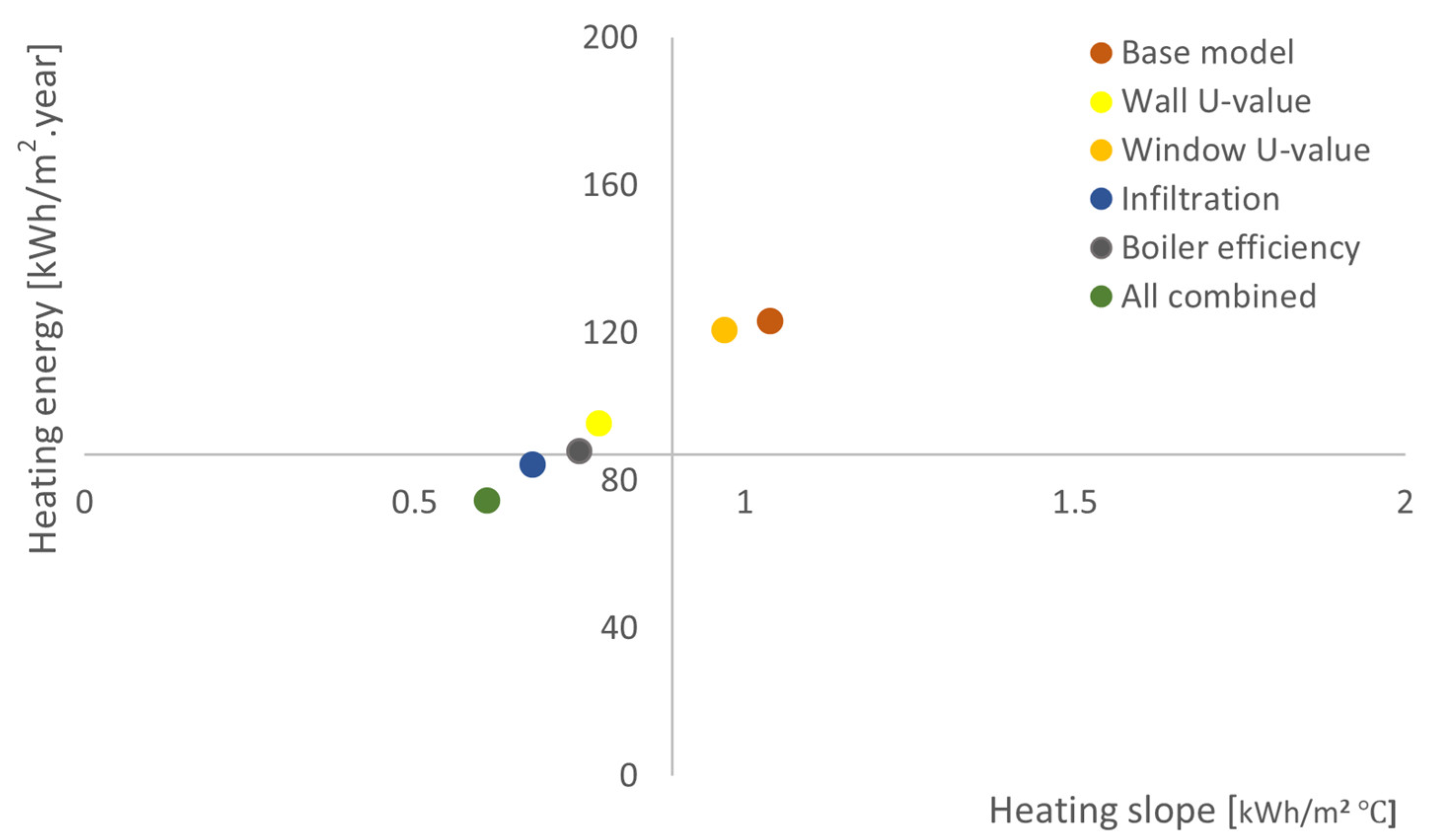
3.3.2. Retrofit Measures and Their Energy Reduction

As mentioned earlier in this study, energy retrofit measures are proposed for house units with a high heating slope and heating energy consumption (first quadrant house units). Hence, measures are selected focusing on the main factors influencing building sensitivity to outdoor temperature variation (envelope thermal properties) and heating energy efficiency. We propose four retrofit measures: improvements in wall and window thermal transmittance (U-value); infiltration rate (ac/h); and boiler efficiency. See

Table 5. Proposed energy-saving measures.

Retrofit Elements	Value
	Base Model	Retrofitted Model
Wall U-value [W/m2 K]	0.72	0.22
Window U-value [W/m2 K]	3.48	1.20
Infiltration ACH50	3.71	0.85
Boiler efficiency	0.70	0.98

for the values related to each suggested measure based on the current energy standards for residential buildings in Republic of Korea. Using the validated base model, we predicted the heating energy consumption from each retrofit measure to calculate change-point regression parameters.

Table 6. Improvement in heating slope and energy consumption from proposed measures.

Simulation Model		${\mathit{S}}_{\mathit{h}}$ [kWh/m2·°C]		${\mathit{E}}_{\mathit{h}}$ [kWh/m2·Year]
		Value	Reduction (%)	Value	Reduction (%)
Base model		1.04	-	123.03	-
Retrofit	Wall	0.78	25.59	95.27	22.57
	Window	0.97	7.36	120.50	2.06
	Infiltration	0.68	34.42	84.16	31.59
	Boiler efficiency	0.75	28.57	87.88	28.57
Four measures combined		0.61	41.44	74.38	39.54

shows the improvements in heating slope and heating energy resulting from the four retrofit measures individually, as well as the improvements based on all the measures combined. Reducing the infiltration rate showed the highest improvement in house unit energy performance, followed by improving the boiler efficiency and wall thermal transmittance. The retrofit measure for window transmittance showed a lower heating energy and slope reduction compared to the other measures. This is due to the small window glazing area and the orientation of the windows. The analyzed house unit is oriented to the south, and during the heating season, solar heat gain contributes to the reduction of energy needed for space heating.

As mentioned in Section 3.2, to classify retrofitted models according to their energy characteristics, we used a four-quadrant plane. As shown in Figure 8, improving a house unit’s infiltration (airtightness) or boiler efficiency can change its energy classification from the first quadrant (energy inefficient) to the third quadrant (high energy performance). A combination of the four measures can be used to further enhance energy performance.

4. Discussion

In this study, we developed a method to characterize and classify the energy consumption of individual house units within apartment complexes. We used a change-point regression model to derive thermal characteristics and energy use features of 200 house units based on their monthly gas consumption. One of the advantages of the change-point regression model is the ability to accurately split weather-dependent energy use (such as heating energy use) and weather-independent energy use (such as energy used for domestic hot water) from monthly energy use data that are easily accessed through utility billing systems [29].

The results in Figure 3 indicate that a three-parameter change-point regression model accurately describes natural gas consumption in house units of apartment complexes in Ulsan, Republic of Korea. Park et al. [14] applied a four-parameter change-point regression model to analyze gas and district heat use of apartment complexes in Seoul, Republic of Korea. In contrast to our study, those authors used monthly energy consumption at the apartment complex level, hence the actual energy use characteristics in individual house units could not be reflected with their model. Generally, in the sampled apartment complexes, when the outdoor temperature exceeded the change-point temperature, consumed gas was only used for weather-independent purposes (such as hot water and cooking), and this energy tended to be constant for a given household. Therefore, a three-parameter change-point regression model for heating can best characterize gas consumption in house units.

According to the change-point regression model results, house units from apartment complex D (built in 2006) showed a relatively lower heating slope (low sensitivity to the outdoor temperature), with an average of 0.77 kWh/m²·°C, while units from apartment complex B (built in 1996) showed an average heating slope of 1.11 kWh/m²·°C. This indicates that improvements in building standards over time influence the overall energy consumption of apartment complexes. Similar results were found in a previous study in Republic of Korea [14]; apartment complexes built after 2003 consumed 61% less heating energy than those built before 2003. In Germany, a study [30] reported a 50% reduction in heating energy in residential buildings from 1978 to 1995.

The variability in the energy characteristics results between house units in the same apartment complex (as shown in Table 2) highlights the need for a practical method to identify and prioritize energy retrofit targets at the individual house unit level, rather than at the apartment complex level. In this study, we used a four-quadrant plane (showing results for both heating slope and heating energy) to classify house units based on their thermal characteristics and their occupant-related features. Through this approach, we identified energy-inefficient house units and assessed potential energy-saving measures.

A building’s thermal properties have a large impact on its energy consumption. Hirst and Goeltz reported that insulation and thermal transmittance are effective energy-saving elements in residential buildings [31]. Santin et al. [32] analyzed energy consumption in residential buildings and attributed 42% of the variation in heating energy use to the heating system and insulation level. Although suggested energy efficiency measures and their energy reductions vary from previous studies in different countries, energy conservation measures that are based on improving building envelopes to minimize heat loss (heating season) and excessive heat gain (cooling season) are the most proposed measures to enhance the energy efficiency of existing buildings.

La Fleur et al. [33] reported that a 44% energy reduction was achieved by a complete renovation of the exterior walls and windows of an apartment in Sweden. In case of a cold climate, the study [34] reported that upgrading the thermal storage of walls in a residential building could reduce its annual energy use by 10 to 24%. The results in our study (Table 6) indicate that improvements in infiltration rate (airtightness), boiler efficiency, and wall transmittance could reduce heating energy consumption by 31.6%, 28.6%, and 22.3%, respectively. Among the proposed measures, improving window transmittance showed the least energy reduction. This finding differs from the results presented in [35] that reported a 7.9 to 16.7% heating energy reduction as a result of improving the window U-value of a detached house by 70%. Nonetheless, our finding is consistent with a previous study conducted at the apartment level [14], where authors reported that retrofits related to window areas had the smallest influence on the variation in heating energy use in the sampled apartment complexes, while the insulation of opaque envelopes showed the largest influence on energy consumption. Various countries are adopting mandatory energy retrofits of existing building stock. Our study contributes insights with regard to identifying energy retrofit targets and assessing efficient measures to improve energy performance in existing buildings. The study’s suggested energy retrofit measures are among the five most essential energy remodeling options desired by private building owners [36]; therefore, their implementation is deemed achievable, especially with current advancements in external insulation methods that enable thermal performance upgrades of a building without the complete replacement of its envelope [37].

5. Conclusions

This study presents a practical method to characterize and classify energy use features of house units within apartment complexes. The study considers 200 house units sampled from five apartment complexes built in different years between 1991 and 2006. Applying the monthly gas consumption of the sampled house units and a change-point regression model, the gas consumption’s dependency on outdoor temperature variations (indicator of a building’s thermal performance) is determined for each house unit. Using the model’s parameters, energy-inefficient house units (targets for energy remodeling) are identified, and potential energy-saving measures are assessed.

The main findings of this study are as follows: (1) Among the five change-point regression models by ASHRAE, a three-parameter model best describes the characteristics of gas consumption of housings in apartment complexes. For all the sampled house units, the regression’s goodness of fit, R², and the coefficient of variation of the root mean squared (CV RMSE) meet the ASHRAE’s guidelines for model applicability. (2) Analyzing the obtained model parameters using a four-quadrant plane allowed us to determine thermal performance and gas consumption characteristics of each house unit. (3) The proposed approach is able to classify house units with a high energy consumption as a result of user-related factors (low heating slope and high heating energy consumption) and house units with poor thermal performance (high heating slope and high heating energy consumption). (4) The assessment of potential energy-saving measures indicate that approximately 30% of heating energy can be saved by improving house insulation or boiler efficiency, and that around 40% of heating energy can be saved by improving insulation, boiler efficiency, and thermal transmittance of the envelope (via walls and windows).

The method applied in this study allows the provision of more detailed information on the energy consumption and thermal performance of buildings; therefore, it can play a crucial role in selecting and prioritizing buildings for implementing large-scale energy upgrades of existing building stock. The analysis performed in this study is based on open data of the monthly gas consumption of house units, and information on other forms of auxiliary heating (such as portable electric heaters) are not included. As result, there are uncertainties in the occupant’s actions that have an influence on the heating energy consumption of a housing unit. Future studies should mitigate these uncertainties by incorporating additional data on heating means used in a house unit as well as the indoor environment, such as indoor temperature. In addition, the amount of actual heating energy from house units may differ as a result of variations in occupant behavior. Predicted energy savings from proposed measures may vary for individual house units; therefore, further work will assess the extent to which user-related factors (such as occupancy patterns and preferences in indoor thermal conditions) impact the findings in this study. Furthermore, future work will apply suggested measures to case studies to quantify their actual energy reductions.

References

1. International Energy Agency (IEA). Available online: https://www.iea.org/reports/transition-to-sustainable-buildings (accessed on 23 July 2024).
2. Amoruso, F.M.; Sonn, M.H.; Chu, S.; Schuetze, T. Sustainable building legislation and incentives in korea: A case-study-based comparison of building new and renovation. Sustainability 2021, 13, 4889. [Google Scholar] [CrossRef]
3. Juan, Y.K.; Hsing, N.P. BIM-based approach to simulate building adaptive performance and life cycle costs for an open building design. Appl. Sci. 2017, 7, 837. [Google Scholar] [CrossRef]
4. Eleftheriadis, G.; Hamdy, M. The impact of insulation and HVAC degradation on overall building energy performance: A case study. Buildings 2018, 8, 23. [Google Scholar] [CrossRef]
5. Wang, E. Benchmarking whole-building energy performance with multi-criteria technique for order preference by similarity to ideal solution using a selective objective-weighting approach. Appl. Energy 2015, 146, 92–103. [Google Scholar] [CrossRef]
6. Lee, W.S.; Lin, L.C. Evaluating and ranking the energy performance of office building using technique for order preference by similarity to ideal solution. Appl. Therm. Eng. 2011, 31, 3521–3525. [Google Scholar] [CrossRef]
7. Singh, V.; Reddy, T.A.; Abushakra, B. Predicting Annual Energy Use in Buildings Using Short-Term Monitoring: The Dry-Bulb Temperature Analysis (DBTA) Method. ASHRAE Trans. 2014, 120, 397–405. [Google Scholar]
8. Abushakra, B.; Paulus, M.T. An hourly hybrid multi-variate change-point inverse model using short-term monitored data for annual prediction of building energy performance, part III: Results and analysis (1404-RP). Sci. Technol. Built Environ. 2016, 22, 996–1009. [Google Scholar] [CrossRef]
9. Afroz, Z.; Gunay, H.B.; O’Brien, W.; Newsham, G.; Wilton, I. An inquiry into the capabilities of baseline building energy modelling approaches to estimate energy savings. Energy Build. 2021, 244, 111054. [Google Scholar] [CrossRef]
10. Do, H.; Cetin, K.S. Evaluation of the causes and impact of outliers on residential building energy use prediction using inverse modeling. Build. Environ. 2018, 138, 194–206. [Google Scholar] [CrossRef]
11. Burak Gunay, H.; Shen, W.; Newsham, G.; Ashouri, A. Detection and interpretation of anomalies in building energy use through inverse modeling. Sci. Technol. Built Environ. 2019, 25, 488–503. [Google Scholar] [CrossRef]
12. Milić, V.; Rohdin, P.; Moshfegh, B. Further development of the change-point model–Differentiating thermal power characteristics for a residential district in a cold climate. Energy Build. 2021, 231, 110639. [Google Scholar] [CrossRef]
13. Kim, K.H.; Haberl, J.S. Development of methodology for calibrated simulation in single-family residential buildings using three-parameter change-point regression model. Energy Build. 2015, 99, 140–152. [Google Scholar] [CrossRef]
14. Park, J.S.; Lee, S.J.; Kim, K.H.; Kwon, K.W.; Jeong, J.W. Estimating thermal performance and energy saving potential of residential buildings using utility bills. Energy Build. 2016, 110, 23–30. [Google Scholar] [CrossRef]
15. Meiss, A.; Padilla-Marcos, M.A.; Feijó-Muñoz, J. Methodology applied to the evaluation of natural ventilation in residential building retrofits: A case study. Energies 2017, 10, 456. [Google Scholar] [CrossRef]
16. Peiris, S.; Lai, J.H.; Kumaraswamy, M.M.; Hou, H.C. Smart retrofitting for existing buildings: State of the art and future research directions. J. Build. Eng. 2023, 76, 107354. [Google Scholar] [CrossRef]
17. Hart, R.; Selkowitz, S.; Curcija, C. Thermal performance and potential annual energy impact of retrofit thin-glass triple-pane glazing in US residential buildings. Build. Simul. 2019, 12, 79–86. [Google Scholar] [CrossRef]
18. Sartori, T.; Calmon, J.L. Analysis of the impacts of retrofit actions on the life cycle energy consumption of typical neighbourhood dwellings. J. Build. Eng. 2019, 21, 158–172. [Google Scholar] [CrossRef]
19. Gugul, G.N.; Koksal, M.A.; Ugursal, V.I. Techno-economical analysis of building envelope and renewable energy technology retrofits to single family homes. Energy Sustain. Dev. 2018, 45, 159–170. [Google Scholar] [CrossRef]
20. Seo, R.S.; Jung, G.J.; Rhee, K.N. Impact of green retrofits on heating energy consumption of apartment buildings based on nationwide energy database in South Korea. Energy Build. 2023, 292, 113142. [Google Scholar] [CrossRef]
21. Korea City Gas Association. Available online: www.citygas.or.kr (accessed on 6 August 2024).
22. Kissock, J.K.; Haberl, J.S.; Claridge, D.E. Inverse modeling toolkit: Numerical algorithms. ASHRAE Trans. 2003, 109, 425. [Google Scholar]
23. Zhang, Y.; O’Neill, Z.; Dong, B.; Augenbroe, G. Comparisons of inverse modeling approaches for predicting building energy performance. Build. Environ. 2015, 86, 177–190. [Google Scholar] [CrossRef]
24. ASHRAE. ASHRAE Handbook—Fundamentals; The American Society of Heating, Refrigerating and Air Conditioning Engineers: Atlanta, GA, USA, 2017. [Google Scholar]
25. Do, H.; Cetin, K.S. Improvement of inverse change-point modeling of electricity consumption in residential buildings across multiple climate zones. Build. Simul. 2019, 12, 711–722. [Google Scholar] [CrossRef]
26. ASHRAE. Ashrae Guideline 14: Measurement of Energy and Demand Savings; The American Society of Heating Refrigerating and Air-Conditioning Engineers: Atlanta, GA, USA, 2002; Volume 35, pp. 41–63. [Google Scholar]
27. Del Ama Gonzalo, F.; Moreno Santamaría, B.; Montero Burgos, M.J. Assessment of building energy simulation tools to predict heating and cooling energy consumption at early design stages. Sustainability 2023, 15, 1920. [Google Scholar] [CrossRef]
28. ASHRAE. ASHRAE Guideline 14-2014: Measurement of Energy, Demand, and Water Savings; The American Society of Heating Refrigerating and Air-Conditioning Engineers: Atlanta, GA, USA, 2014; Volume 4, pp. 1–150. [Google Scholar]
29. Haberl, J.S.; Cho, S. Literature Review of Uncertainty of Analysis Methods, (DOE-2 Program), Report to the Texas Commission on Environmental Quality. Available online: https://hdl.handle.net/1969.1/2072 (accessed on 16 May 2024).
30. Schuler, A.; Weber, C.; Fahl, U. Energy consumption for space heating of West-German households: Empirical evidence, scenario projections and policy implications. Energy Policy 2000, 28, 877–894. [Google Scholar] [CrossRef]
31. Hirst, E.; Goeltz, R. Comparison of actual energy savings with audit predictions for homes in the north central region of the USA. Build. Environ. 1985, 20, 1–6. [Google Scholar] [CrossRef]
32. Santin, O.G.; Itard, L.; Visscher, H. The effect of occupancy and building characteristics on energy use for space and water heating in Dutch residential stock. Energy Build. 2009, 41, 1223–1232. [Google Scholar] [CrossRef]
33. La Fleur, L.; Moshfegh, B.; Rohdin, P. Measured and predicted energy use and indoor climate before and after a major renovation of an apartment building in Sweden. Energy Build. 2017, 146, 98–110. [Google Scholar] [CrossRef]
34. Soares, N.; Gaspar, A.R.; Santos, P.; Costa, J.J. Multi-dimensional optimization of the incorporation of PCM-drywalls in lightweight steel-framed residential buildings in different climates. Energy Build. 2014, 70, 411–421. [Google Scholar] [CrossRef]
35. Ahn, B.L.; Kim, J.H.; Jang, C.Y.; Leigh, S.B.; Jeong, H. Window retrofit strategy for energy saving in existing residences with different thermal characteristics and window sizes. Build. Serv. Eng. Res. Technol. 2016, 37, 18–32. [Google Scholar] [CrossRef]
36. Benzar, B.E.; Park, M.; Lee, H.S.; Yoon, I.; Cho, J. Determining retrofit technologies for building energy performance. J. Asian Archit. Build. Eng. 2020, 19, 367–383. [Google Scholar] [CrossRef]
37. Lee, H.; Choi, G.S. Analysis of the Energy Consumption of Old Public Buildings in South Korea after Green Remodeling. Buildings 2023, 13, 3081. [Google Scholar] [CrossRef]
Figure 1. Floor plan of house units from the four apartment complexes: floor plan for (a) A, (b) B, (c) C, and (d) D apartment complex.
Energies 17 04186 g001
Figure 2. Three-parameter change-point heating model.
Energies 17 04186 g002
Figure 3. Monthly gas consumption of a housing unit plotted against the outdoor temperature utilizing a three-parameter change−point regression model.
Energies 17 04186 g003
Figure 4. Distribution of the results from the change-point regression model: (a) heating slope; (b) change-point temperature; and (c) heating energy. The curve lines indicate similar trend in variations of the obtained heating slope and heating energy.
Energies 17 04186 g004
Figure 5. Heating slope and energy consumption of sampled house units in a four-quadrant plane.
Energies 17 04186 g005
Figure 6. DesignBuilder/EnergyPlus model of the analyzed house unit from apartment complex B.
Energies 17 04186 g006
Figure 7. Comparison between actual heating energy and heating energy predicted from the base model.
Energies 17 04186 g007
Figure 8. Improvement in energy performance due to retrofitting measures shown in a four-quadrant plane.
Energies 17 04186 g008