Research on Low-Carbon Building Development and Carbon Emission Control Based on Mathematical Models: A Case Study of Jiangsu Province

Abstract

This paper investigates the development of low-carbon buildings and carbon emission control in Jiangsu Province, China, utilizing a mathematical model. Through correlation analysis and principal component analysis, the carbon emissions of the entire life cycle of residential buildings are evaluated, and a Grey Prediction Model is established. The study shows that the annual carbon emission from air conditioners is 370.92 kg, given an annual electricity consumption of 1324.71 kW and a carbon emission of 0.28 kg per kWh. It identifies the key carbon emission indicators, including precipitation, temperature, energy consumption, building area, construction materials, water, natural gas, and waste. Principal component analysis ranks building area as the most significant factor. Using the GM (1,1) model, the carbon emissions of Jiangsu Province in 2024 were predicted to be 1.5576 million tons by historical data. Emission reduction suggestions are proposed, such as constructing thicker walls, increasing green spaces, reducing construction waste, and promoting balanced economic development. Moreover, prioritizing insulation materials in building design can reduce winter energy consumption since energy consumption is higher in winter than in summer. This research supports China’s goals of achieving a carbon peak by 2030 and carbon neutrality by 2060 while encouraging low-carbon technological innovation and improving people’s living standards. This study also emphasizes the importance of locally tailored strategies for effective emissions reduction.

1. Introduction

1.1. Background

Amid the worsening global climate change, China has set ambitious goals to peak carbon emissions by 2030 and achieve carbon neutrality by 2060. In line with national policies and to foster low-carbon development, the construction industry must expedite its efforts to reduce carbon emissions. Low-carbon buildings have become a focal point in this initiative, aiming to minimize the use of fossil fuels, enhance energy efficiency, and reduce carbon dioxide emissions by optimizing building materials, equipment manufacturing, construction processes, and building usage throughout their lifecycle.

To promote the development of low-carbon buildings, China is actively advancing green and low-carbon technological innovations to boost the global competitiveness of its industry and economy. In the construction sector, these innovations encompass architectural design, energy-saving technologies, and the application of renewable energy. By leveraging innovative technological methods, it is possible to improve the energy efficiency of buildings, reduce reliance on traditional energy sources, and enhance the comfort and sustainability of buildings.

This paper aims to study the development of low-carbon buildings and explore methods to reduce carbon emissions throughout the lifecycle of building materials, equipment manufacturing, construction processes, and building usage. The goal of analyzing key technologies and policy measures for low-carbon buildings and evaluating their environmental and economic impacts is to propose effective strategies and measures for reducing carbon emissions in buildings. This will provide a scientific basis and guidance for achieving the “dual carbon” goals and promote the transformation of China’s construction industry towards a green, environmentally friendly, and low-carbon lifestyle.

1.2. Model Assumptions and Problems

Traditionally, heat conduction models have been primarily used in physics and engineering to study heat conduction phenomena. This paper innovatively applies the heat conduction model to energy loss assessment and proposes design solutions to optimize energy consumption. By comprehensively considering factors such as the physical properties of materials, modes of heat conduction, and time, this approach helps designers make more precise and effective optimizations in energy utilization, thereby enhancing energy efficiency. This paper aims to solve various carbon emission problems based on a single-story, flat-roofed mono-building by establishing mathematical models [1]. Our goal is to calculate the carbon emissions from temperature regulation through air conditioning in a single-story, flat-roofed mono-building measuring 4 m in length, 3 m in width, and 3 m in height over the course of one year. The building’s walls are brick-concrete structures with a thickness of 30 cm; the roof is poured reinforced concrete, also with a thickness of 30 cm; the total area of doors and windows is 5 square meters; and the ground is concrete. The geographical location of the building has average monthly temperature data for 12 months. Based on the above assumptions, the indoor temperature of the building needs to be maintained between 18 and 26 °C. When the temperature is not suitable, electricity is used to regulate it, with one unit of electricity consumption equating to 0.28 kg of carbon emissions. In addition, the heating Coefficient of Performance (COP) of the air conditioner is 3.5, and the cooling Coefficient of Performance (EER) is 2.7. This problem will be calculated based on the above conditions to determine the carbon emissions caused by temperature regulation through air conditioning in the building over the course of one year [2]. Furthermore, factors that are highly correlated and easily quantifiable with the above conditions will be identified to comprehensively evaluate carbon emissions throughout the lifecycle of residential buildings. Additionally, the effectiveness of the established evaluation model will be verified to ensure its reliability. Using the established model and historical data on the lifecycle carbon emissions of buildings in Jiangsu Province, a forecast will be made for the building lifecycle carbon emissions in the province for 2024 [3]. Policy recommendations for carbon emission reduction in Jiangsu Province’s buildings will also be proposed. These recommendations will be based on the research results and model analysis mentioned above, aiming to promote the low-carbon development of Jiangsu Province’s construction industry and provide important references for emission reduction policy formulation and low-carbon building design. As one of China’s major economic provinces, Jiangsu Province has a strong industrial foundation and a rapid urbanization process. Therefore, the study of low-carbon development in Jiangsu Province’s construction industry is both representative and significant. By researching Jiangsu Province, it can provide strong support and innovative contributions to energy conservation and emission reduction across the country. Applying the models described in this article to the total construction area in Jiangsu Province, the annual reduction in carbon dioxide emissions will reach 4.05 million tons. At the same time, the application area of renewable energy buildings will reach 5 million square meters, reducing carbon dioxide emissions by about 500,000 tons annually.

Combining China’s national conditions with Carbon Capture, Utilization, and Storage (CCUS) technology and low-carbon construction practices can significantly reduce the carbon footprint of the construction industry. An innovative three-step approach for the national promotion of CCUS has been designed. The phased implementation of CCUS technology can effectively integrate resources and optimize its application in the construction industry.

First, during the industry pilot phase (2021–2030), the government should introduce subsidy policies and tax reductions to provide economic incentives and operational guarantees for the application of CCUS technology in the construction industry. At the same time, it should assess R&D investment according to the 2050 emission reduction target and plan resources accordingly [4].

Second, during the regional promotion phase (2031–2040), each region should formulate suitable CCUS application roadmaps, increase support for technology application, and promote its widespread use through subsidies and policies.

Finally, during the national application phase (after 2040), the nationwide deployment of CCUS should be promoted in an orderly manner by identifying resource integration opportunities, optimizing the value chain, achieving cost synergies, gradually phasing out subsidies, and drawing on successful experiences from other regions.

Combining CCUS technology with the low-carbon construction industry, through the joint efforts of the government and enterprises, multi-mechanism and cross-industry cooperation will be achieved to realize a low-carbon, clean, efficient, and safe new energy system, accelerating the achievement of carbon neutrality strategic goals [5].

2. Methods

To investigate the annual carbon emissions from temperature regulation through air conditioning in buildings, we conducted the following study. Firstly, considering that air conditioning operates in three modes (cooling, heating, and not in use), we divided the twelve months into three parts: the first part is from November to April, requiring heating mode; the second part is from June to August, requiring cooling mode; the third part is May, September, and October, where no air conditioning is needed. For temperatures exceeding 26 °C, the temperature is adjusted to 26 degrees; for temperatures below 18 °C, the temperature is adjusted to 18 degrees. We assume that the thickness of the ground is consistent with that of the walls and roof, all being 30 cm, and neglect the influence of the small door and window areas. By calculating the heat conduction heat flux of the building through the relationship between the heat exchange power between the building and the external environment and the thermal conductivity coefficient, contact area, thickness, and temperature difference, and then calculating the working power of the air conditioning system through the ratio of heat flux to the heating (cooling) performance coefficient, we further deduce the energy consumption of air conditioning and thus obtain the annual carbon emissions. To study the impact of indicators involved in the comprehensive evaluation of carbon emissions throughout the lifecycle of residential buildings, this paper conducted research during the construction, operation, and demolition phases. We collected annual data on carbon emissions from residential buildings nationwide from 2018 to 2023 and selected ten indicators covering important influencing factors during the construction, operation, and demolition phases [6]. Through correlation analysis, we assessed whether these indicators were related to carbon emissions and used Principal Component Analysis (PCA) to reduce the dimensionality of the data. By assigning weights to different principal components based on their contribution rates, we gradually determined the importance of each indicator to carbon emissions.

A comprehensive evaluation of carbon emissions from residential buildings in thirteen prefecture-level cities in Jiangsu Province in 2021 was conducted, analyzing the relevant results and considering emission issues related to the three stages of the building lifecycle. Relevant indicators for the three stages of the building lifecycle were identified, and PCA was applied to these indicators. Using Matlab 2024a, correlation heatmaps were created to observe the correlation between indicators and reduce the dimensionality of the indicators. Finally, the main components were determined, and weights were assigned based on the contribution rates of the principal components to calculate the comprehensive scores of the thirteen prefecture-level cities in terms of carbon emissions from residential buildings [7].

To forecast the carbon emissions from the entire lifecycle of buildings in Jiangsu Province in 2024, research was conducted based on historical data on the carbon emissions from the entire lifecycle of buildings in Jiangsu Province. Relevant literature was reviewed to obtain data on the carbon emissions from residential buildings in Jiangsu Province over the years, and the grey prediction method was used to forecast the carbon emissions from residential buildings over the years. Through this method, the forecast results of the carbon emissions from the entire lifecycle of buildings in Jiangsu Province in 2024 were obtained. Suggestions were also proposed to improve these indicators to increase the low-carbon level of urban buildings.

2.1. Model Assumptions

Given the actual circumstances of this problem, to ensure the accuracy and rationality of the model solution, we make the following assumptions during the analysis:

• The data collected for this study are all reliable and valid. However, we do not consider the existence of other uncertain factors. The uncertain factors are limited to those mentioned in the text and do not include other potential sources of uncertainty.
• We assume that the area of doors and windows has no effect on the calculation of building energy consumption.
• We assume that extreme factors are not considered when calculating the heat loss of the building.
• We assume that when calculating the energy consumption of temperature regulation, the temperature adjustment by air conditioning will not exceed 18 °C or fall below 26 °C.

2.2. Symbol Explanation

For clarity, the following symbols are used in this paper (see

Table 1. Symbol explanation.

Symbols	Explanation
$\mathsf{\Delta }T$	Indoor-outdoor temperature difference
$S$	Heat transfer area
$q$	Air conditioning power
$Q$	Heat flux
$L$	Thickness of the heat transfer layer
$M$	Air conditioning consumption
$\epsilon (k)$	Residual
$\lambda (k)$	Ratio of levels
$x^1$	Accumulate the data in turn
$x^0$	Raw data

).

3. Establishment and Solution of the Model

After the above analysis and preparation, this paper will gradually establish the following mathematical models to further illustrate the practical process of model establishment.

The mathematical model of a single-story, flat-roofed mono-building is as follows:

The building is 4 m long, 3 m wide, and 3 m high, with a relevant brick and concrete structure thickness of 30 cm. The total area of doors and windows is 5 square meters. There are differences in the thermal conductivity coefficients at different locations. The thermal conductivity coefficient of the walls is 0.3 w/m²·k, and the thickness is 30 cm and the area is 37 square meters. The thermal conductivity of the roof is 0.2 w/m²·k. The thermal conductivity of the ground is 0.25 w/m²·k.

When the temperature is below 18 °C, the monthly heat loss is calculated as follows:

Heat loss = (wall area × wall thermal conductivity + roof area × roof thermal conductivity + total area of doors and windows × thermal conductivity of doors and windows + ground area × ground thermal conductivity) × (18—average monthly temperature) electricity consumption = heat loss/heating performance coefficient (COP) carbon emissions = electricity consumption × 0.28.

When the temperature is above 26 °C, the monthly heat gain is calculated as follows:

Heat gain = (wall area × wall thermal conductivity + roof area × roof thermal conductivity + total area of doors and windows × thermal conductivity of doors and windows + ground area × ground thermal conductivity) × (average monthly temperature—26); electricity consumption = heat gain/cooling performance coefficient (EER) carbon emissions = electricity consumption × 0.28.

When the temperature is between 18 and 26 °C, both electricity consumption and carbon emissions are 0.

3.1. Heat Transfer Model

3.1.1. Calculate the Heat Flow

The formula for calculating the heat flux of building heat transfer is as follows:

$$Q_i={\displaystyle \frac{k\times S\times \mathsf{\Delta }T}{t}}$$

(1)

Here, k represents the thermal conductivity, indicating the amount of heat transferred per unit time per unit area when the temperature difference between the air on both sides of the structure is 1 degree under steady heat transfer conditions; A is the heat transfer area; d is the thickness of the heat transfer layer; ΔT is the temperature difference between indoor and outdoor, Q is the heat flux of building heat transfer.

Using Matlab to calculate the heat flux loss per unit time in January, February, March, April, November, and December, and the heat flux increase per unit time in June, July, and August (see

Table 2. Internal and external heat flux.

Months	Heat Flux Loss (Joules)	Month	Increase in Heat Flux (Joules)
1	1551.7	6	163
2	1306.7	7	408.3
3	980	8	490
4	490
11	245
12	1306.7

).

3.1.2. Calculate the Amount of Electricity Consumed per Month

The power (W) formula required by an air conditioner to maintain a house temperature of 18–26 °C is as follows:

$$q_1={\displaystyle \frac{Q}{COP}}$$

(2)

$$q_2={\displaystyle \frac{Q}{EER}}$$

(3)

COP represents the coefficient of heating performance, which indicates the heat output produced per unit of power input. It is an important indicator of the efficiency of heating equipment; the higher the COP value, the higher the heating efficiency of the equipment. EER stands for the Energy Efficiency Ratio of cooling and indicates the amount of cooling output produced per unit of power input. It is an important indicator for measuring the efficiency of cooling equipment; the higher the EER value, the higher the cooling efficiency of the equipment. The formula for calculating monthly electricity consumption is as follows: q × 3600 × 24 × the number of days in the month.

Using Matlab to calculate the power (in kW) required to maintain the house temperature between 18 and 26 °C for each month from January to December (see

Table 3. Monthly power consumption.

Month	Energy Consumption For Heating (Wh)	Month	Energy Consumption for Cooling (Wh)
1	319.2	6	43.6
2	268.8	7	108.9
3	201.6	8	130.7
4	100.8
11	504

).

For calculating the carbon emissions, the electricity consumption of the air conditioner to maintain the house temperature between 18 and 26 °C is given by the following:

$$M=Q\times 24\times 30$$

(4)

The carbon emissions (kg) are calculated as follows:

$$H=M\times 0.28$$

(5)

where the air conditioner operates 24 h a day, and the number of days in a month is assumed to be 30.

Using Matlab to calculate the carbon emissions (in kg) required to maintain the house temperature between 18 and 26 °C for each month from January to December (see Figure 1,

Table 4. Monthly carbon emissions.

Month	Carbon Emissions for Heating	Month	Carbon Emissions for Cooling (kg)
1	92.3552	6	12.1956
2	70.2464	7	31.
3	58.3296	8	37.8062
4	28.2240
11	14.1120
12	77.7728

).

According to the research literature, we conducted an analysis of the factors influencing carbon emissions during the entire lifecycle of residential buildings, including the construction, operation, and demolition stages [8]. The results are as follows (see Figure 2).

Based on this figure, we can simply summarize it into the construction stage, the usage stage, and the demolition stage, as shown in Figure 3.

From the data in the chart, it can be concluded that in the entire lifecycle of residential buildings globally, the operational stage has the highest proportion of carbon emissions, followed by the construction stage. In contrast, the demolition stage has the lowest proportion of carbon emissions [9].

The entire lifecycle of residential buildings includes three stages: construction, operation, and demolition. The key indicators selected for these three stages are as follows (see Figure 4).

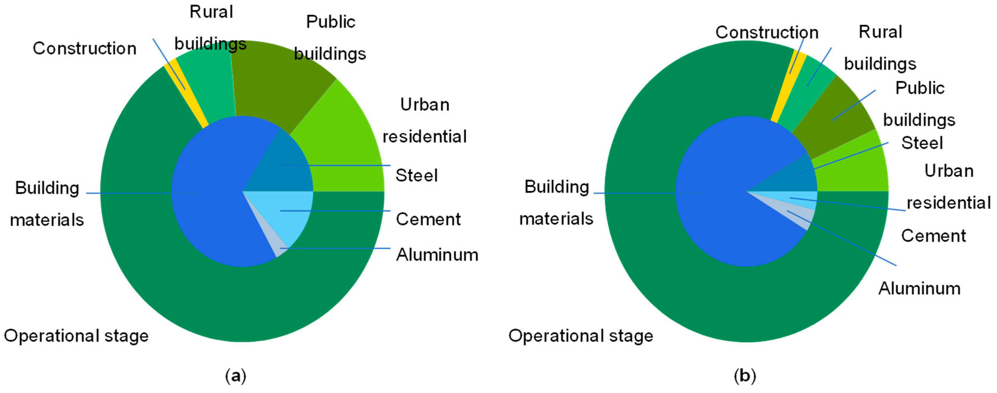
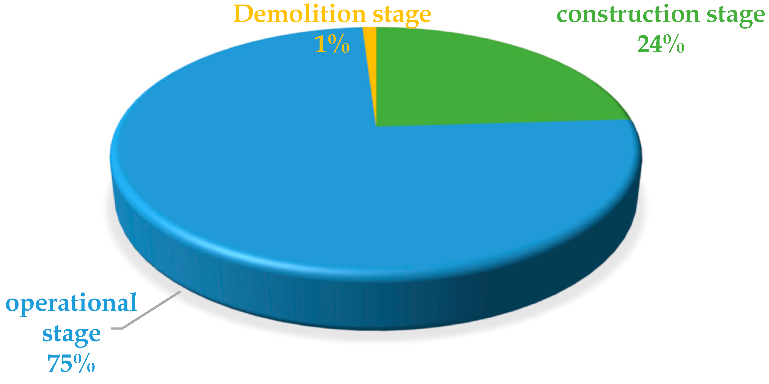
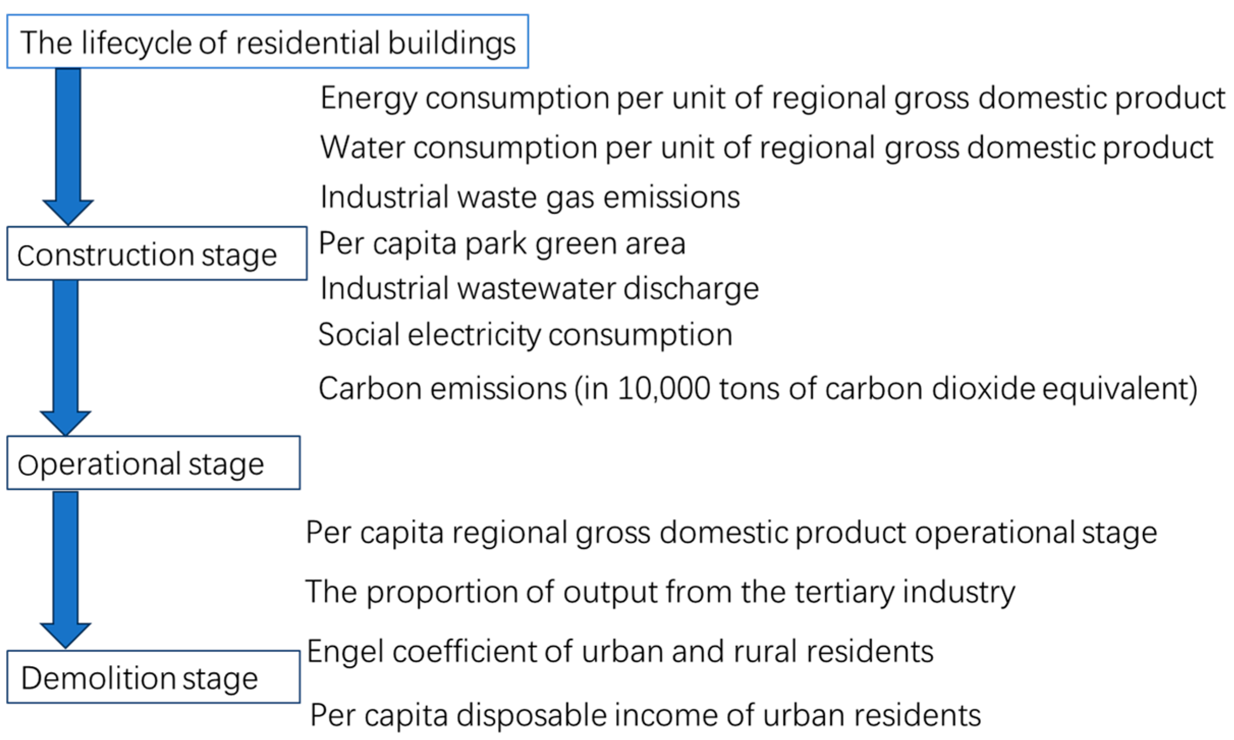
3.2. Lifecycle of Buildings

3.2.1. Analysis of Various Indicators and Data in the Lifecycle of Buildings

The team checked the official websites of the National Bureau of Statistics and the Ministry of Construction to collect data for the ten indicators in China from 2018 to 2023. The specific sources of data are as follows: the Statistical Bulletin on National Economic and Social Development of Jiangsu Province, the Jiangsu Provincial Bureau of Statistics, and the Survey Office of the National Bureau of Statistics in Jiangsu [10] (see

Table 5. Relevant building data.

Years	2018	2019	2020	2021	2022	2023
Per capita regional gross domestic product	44,253	52,840	62,290	68,347	75,354	81,874
The proportion of output from the tertiary industry	39.6	41.4	42.4	43.5	45.5	47
Energy consumption per unit of regional gross domestic product	0.86	0.81	0.72	0.69	0.62	0.56
Water consumption per unit of regional gross domestic product	21.71	17.4	14.09	13.03	11.66	9.71
Industrial waste gas emissions	34,154	31,213	48,183	48,623	49,797	59,652
Engel coefficient of urban and rural residents	36.3	36.5	36.1	35.4	34.7	34
Per capita disposable income of urban residents	20,552	22,944	26,341	29,677	32,538	35,248
Per capita park green area	13.2	13.3	13.3	13.6	14	14.4
Industrial wastewater discharge	27.65	26.38	24.63	23.61	22.06	20.49
Total energy consumption	23,709	25,774	27,589	28,850	29,205	29,863
Social electricity consumption	3314.0	3864.37	4281.62	4580.9	4956.62	5012.54
Carbon emissions (in 10,000 tons of carbon dioxide equivalent)	115.2	121.6	128.1	134.5	132.65	137.6

).

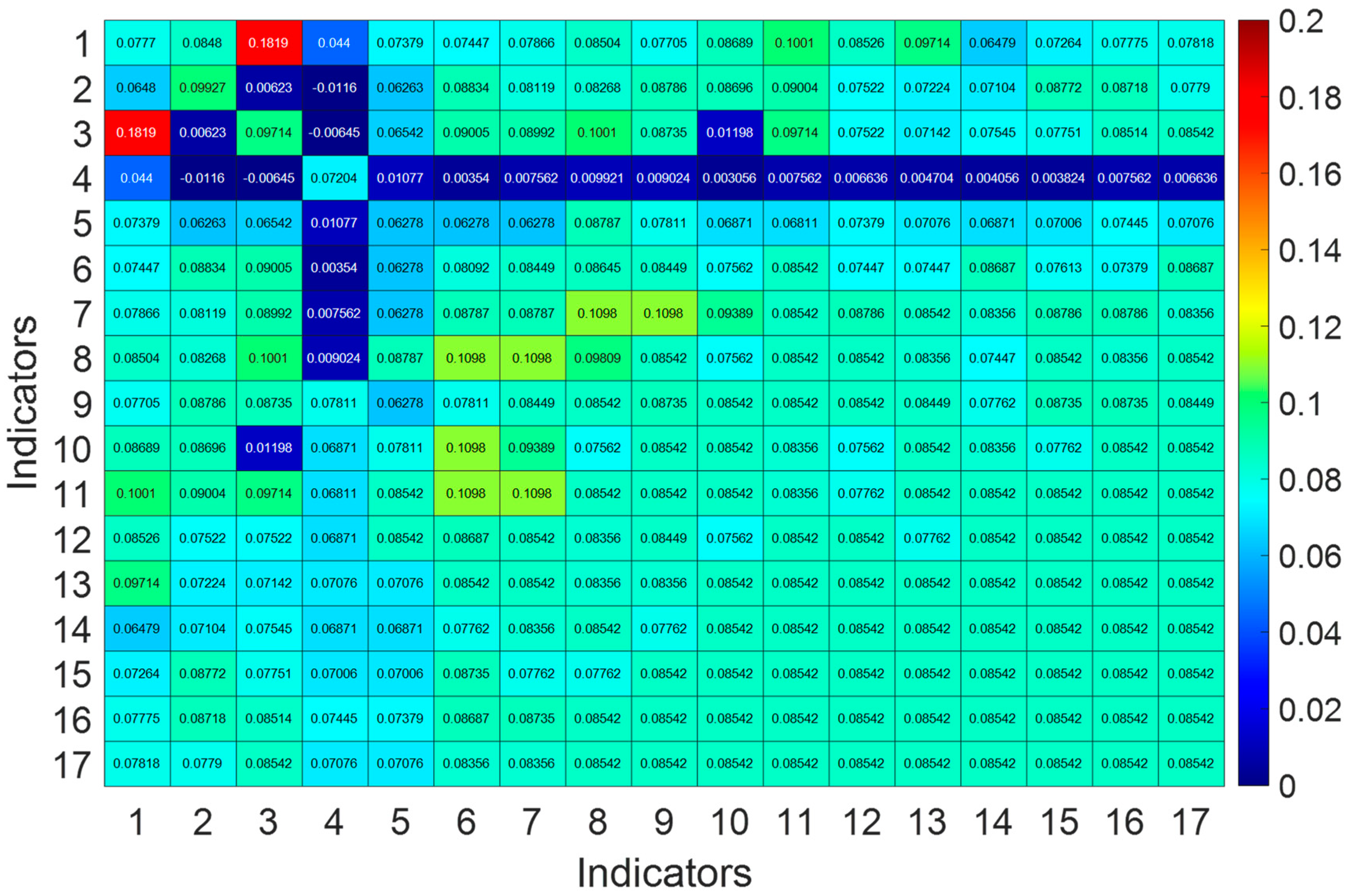
3.2.2. Correlation Analysis of Indicators

Correlation analysis was conducted on the collected indicators to determine if Principal Component Analysis (PCA) could be applied to the data. Using Matlab, the correlation (r) between building carbon emissions and each indicator was calculated. The specific results are shown in the table below (see

Table 6. Indicators.

Indicators
Per capita regional gross domestic product
The proportion of output from the tertiary industry
Energy consumption per unit of regional gross domestic product
Water consumption per unit of regional gross domestic product
Industrial waste gas emissions
Engel coefficient of urban and rural residents
Per capita disposable income of urban residents
Per capita park green area
Industrial wastewater discharge
Total energy consumption

).

3.3. Data Collection

3.3.1. Data on Carbon Emissions

The table below presents partial data on carbon emissions and average values of various indicators for thirteen prefecture-level cities in Jiangsu Province up to 2023, based on information collected from sources like the National Bureau of Statistics (see

Table 7. Data on carbon emissions and related indicators of residential buildings in 13 prefecture-level cities.

City Names	Per Capita Local Fiscal Revenue	Average Energy Consumption Level of Buildings
Suqian	4489	88.23
Lianyungang	5996	144.99
Yancheng	2348	45.09
Huai’an	2830	126.3
Yangzhou	3282	129.22
Taizhou	3811	134.91
Xuzhou	5686	179.73
Nantong	3409	12.32
Wuxi	8529	269.595
Suzhou	12,509.2	395.406
Changzhou	6254.6	197.703
Nanjing	11,372	359.46
Zhengjiang	6823.2	215.676

, Figure 5).

The correlation heatmap shows some degree of correlation between various indicators, although the correlation is not very strong. Therefore, Principal Component Analysis (PCA) can be employed.

3.3.2. Establishment of Principal Component Analysis (PCA) Model

1.

Standardize the relevant data. The specific formula is as follows [11,12,13,14,15,16,17,18,19,20,21]:

$$\overline{X}={\displaystyle \frac{1}{n}}\sum _{i=1}^n{X}_{ij};\overline{Y}=\sqrt{{\displaystyle \frac{1}{n-1}}\sum _{i=1}^n(X_{ij}-\overline{X}{)}^2},i=\mathrm{1,2},\dots ,13;j=\mathrm{1,2},\dots ,17$$

(6)

$${\overline{X}}_{ij}={\displaystyle \frac{X_{ij}-\overline{X}}{{\overline{Y}}_j}}$$

(7)

where $X_{ij}$ is the j-th value of the i-th city; ${\overline{X}}_j$ and ${\overline{Y}}_j$ is the j-th sample average and standardized value, respectively

Using Matlab to calculate the standardized value, the following is a partial dataset (see

Table 8. Standardized data.

City Names	Per Capita Local Fiscal Revenue	Average Energy Consumption Level of Buildings
Suqian	−0.4561	−0.7883
Lianyungang	0.0146	−0.2832
Yancheng	−1.1248	−1.1722
Huai’an	−0.9743	−0.4495
Yangzhou	−0.8331	−0.4236
Taizhou	−0.6679	−0.3729
Xuzhou	−0.0822	0.0259
Nantong	−0.7934	−1.4638
Wuxi	0.8058	0.8256
Suzhou	2.0491	1.9451
Changzhou	0.0954	0.1858
Nanjing	1.6939	1.6252
Zhengjiang	0.2730	0.3458

).

2.

Calculate eigenvalues, eigenvectors, and cumulative contribution rates.

Calculate the relevant eigenvalues, eigenvectors, cumulative contribution rates, variance percentages, cumulative percentages, and factor loading coefficients using Matlab based on the standardized data. The following is a partial dataset (see

Table 9. Total variance explained.

Components		1	2	3
Initial eigenvalues	Variance percentage	52.2742	14.8430	14.0133
	Cumulative percentage	52.2742	67.1172	81.1306
	Cumulative contribution rate	0.5227	0.6712	0.8113
Loadings Sum of squares	Variance percentage	52.2742	14.8430	14.0133
	Cumulative percentage	52.2742	67.1172	81.1306
	Cumulative contribution rate	0.5227	0.6712	0.8113

).

According to the table above, it can be observed that the cumulative contribution rates of the first three principal components are all greater than 80% in the variance explanation table. Therefore, three principal components can be selected.

3.

Calculate the component matrix.

Using Matlab software, calculate the relevant component score coefficients. The specific data is shown in the table below (see

Table 10. Component score coefficient matrix.

Components	1	2	3
index1	3.2612	1.4835	0.3786
index2	1.0681	−0.3577	0.7418
index3	0.0047	−0.8499	0.6085
index4	−8.0916	3.0670	0.5311
index5	0.6725	−0.9635	4.1067
index6	−1.7564	−1.5859	0.6761
index7	−1.8565	−1.7575	−0.1495
index8	−0.6674	−0.5120	−0.4241
index9	−2.1221	−2.0543	−1.1509
index10	−0.2323	−0.1805	−0.2169
index11	0.7763	−0.3014	−0.8577
index12	1.1221	0.2972	−0.1317
index13	2.9553	2.3608	0.0544
index14	0.7408	0.2869	−1.6175
index15	0.2154	−0.0338	−2.0594
index16	2.5291	1.2314	0.5227
index17	1.3808	−0.1254	−0.9944

).

The values of the seventeen indicators corresponding to index1, index2, …, index17 cities can be used to calculate the component score coefficients for each principal component using the following formula.

$$\begin{array}{cc}{{\displaystyle Y}}_1& =3.2612{{\displaystyle x}}_1+1.0681{{\displaystyle x}}_2+0.0047{{\displaystyle x}}_3-8.0916{{\displaystyle x}}_4+0.6725{{\displaystyle x}}_5-{{\displaystyle 1.7564x}}_6-1.8565x_7{{\displaystyle -0.6674x}}_8-2.1221{{\displaystyle x}}_9\\ & -0.2323{{\displaystyle x}}_{10}+0.7763{{\displaystyle x}}_{11}+{{\displaystyle 1.1221x}}_{12}+{{\displaystyle 2.9553x}}_{13}+{{\displaystyle 0.7408x}}_{14}+{{\displaystyle 0.2154x}}_{15}+{{\displaystyle 2.5291x}}_{16}+1.3808{{\displaystyle x}}_{17}\end{array}$$

$$\begin{array}{cc}{{\displaystyle Y}}_2& =1.4835{{\displaystyle x}}_1-0.3577{{\displaystyle x}}_2-0.8499{{\displaystyle x}}_3+3.0670{{\displaystyle x}}_4-0.9635{{\displaystyle x}}_5-1.5859{{\displaystyle x}}_6-1.7575{{\displaystyle x}}_7-0.5120{{\displaystyle x}}_8-2.0543{{\displaystyle x}}_9\\ & -0.1805{{\displaystyle x}}_{10}-0.3014{{\displaystyle x}}_{11}+0.2972{{\displaystyle x}}_{12}+2.3608{{\displaystyle x}}_{13}+0.2869{{\displaystyle x}}_{14}-0.0338{{\displaystyle x}}_{15}+1.2314{{\displaystyle x}}_{16}-0.1254{{\displaystyle x}}_{17}\end{array}$$

$$\begin{array}{cc}{{\displaystyle Y}}_3& =0.3786{{\displaystyle x}}_1+0.7418{{\displaystyle x}}_2+0.6085{{\displaystyle x}}_3+0.5311{{\displaystyle x}}_4+4.1067{{\displaystyle x}}_5+0.6761{{\displaystyle x}}_6-0.1495{{\displaystyle x}}_7-0.4241{{\displaystyle x}}_8-1.1509{{\displaystyle x}}_9\\ & -0.2169{{\displaystyle x}}_{10}-0.8577{{\displaystyle x}}_{11}+0.1317{{\displaystyle x}}_{12}+0.0544{{\displaystyle x}}_{13}-1.6175{{\displaystyle x}}_{14}-2.0594{{\displaystyle x}}_{15}+0.0527{{\displaystyle x}}_{16}-0.9944{{\displaystyle x}}_{17}\end{array}$$

4.

Calculate composite score coefficients.

According to

$$Y={\displaystyle \frac{52.2742}{134.1308}}\times Y_1+{\displaystyle \frac{14.8430}{134.1308}}\times Y_2+{\displaystyle \frac{14.0133}{134.1308}}\times Y_3$$

(8)

the composite scores of carbon emissions for the thirteen prefecture-level cities in Jiangsu Province are calculated. The specific results are shown in the table below [20,22,23,24] (see

Table 11. Composite score coefficients.

City Names	Components 1	Components 2	Components 3	Composite Score
Suqian	1.1138 × 105	7.7466 × 104	2.2723 × 104	5.4354 × 104
Lianyungang	1.3088 × 105	8.3038 × 104	2.5300 × 104	6.2840 × 104
Yancheng	−1.7376 × 104	9.7685 × 103	4.7785 × 103	5.1916 × 104
Huai’an	−2.6447 × 105	1.6799 × 105	3.5142 × 104	8.0809 × 104
Yangzhou	1.2701 × 105	8.4893 × 104	2.2999 × 104	6.1296 × 104
Taizhou	1.3480 × 105	9.3617 × 104	2.5243 × 104	6.5532 × 104
Xuzhou	1.7486 × 105	1.0211 × 105	2.9811 × 104	8.2561 × 104
Nantong	8.5770 × 104	6.2991 × 104	1.8643 × 104	4.2345 × 104
Wuxi	2.6230 × 105	1.5316 × 105	4.4716 × 104	1.2385 × 105
Suzhou	3.8470 × 105	2.2464 × 105	6.5584 ×104	1.8164 × 105
Changzhou	1.9235 × 105	1.1232 ×105	3.2792 × 104	9.0819 × 104
Nanjing	3.4973 × 105	2.0422 × 105	5.9621 × 104	1.6513 × 105
Zhengjiang	2.0984 × 105	1.2253 × 105	3.5773 × 104	9.9077 × 104

, Figure 6).

Based on the evidence above, it can be inferred that Suzhou City in Jiangsu Province has the highest comprehensive score of 1.61568. Therefore, Suzhou has the highest carbon emissions in the construction process in Jiangsu, followed by Nanjing, Wuxi, and Zhenjiang. Yancheng has the lowest carbon emissions in the entire construction process, followed by Suqian and Yangzhou.

3.4. Establishment of Grey Prediction Model

1.

The Grey Prediction Model is suitable for situations with a small sample size and relatively low computational workload. This is advantageous for the case of the total carbon emissions from buildings in Jiangsu Province for the years 2016–2023, where the sample size is not large. The Grey Prediction Model establishes grey differential equations to predict future trends based on existing data, providing a reference for prediction results. Although long-term predictions may have some errors, the Grey Prediction Model still offers a quick and effective method in situations with insufficient sample size.

Level Ratio Test:

Establish the time series of residential building carbon emissions in Jiangsu Province as follows:

$$x^{\left(0\right)}=\left[x^{\left(0\right)}\left(1\right),x^{\left(0\right)}\left(2\right),L,x^{\left(0\right)}\left(8\right)\right]=(102.3,108.7,115.2,121.6,128.1,134.5,140.96,147.41)$$

(9)

(1).

Calculate the level ratio,

$$\lambda \left(k\right)={\displaystyle \frac{x^{\left(0\right)}\left(k-1\right)}{x^{\left(0\right)}\left(k\right)}}$$

(10)

where

$$\lambda =\left[\lambda \left(2\right),\lambda \left(3\right),\cdots ,\lambda \left(8\right)\right]=\left(0.9411,0.9436,0.9474,0.9493,0.9524,0.9542,0.9562\right)$$

(11)

(2).

Level ratio test graph (see Figure 7):

Through relevant judgments, it is found that:

$$\lambda \left(k\right)\in \left(e^{{\displaystyle \frac{-2}{n+1}}},e^{{\displaystyle \frac{2}{n+1}}}\right)=\left[0.8007,1.2488\right]$$

(12)

2.

GM(1,1) Model:

In this study, the GM (1,1) model from the grey system theory was used to make a prediction. The first “1” means univariate, i.e., the model uses only one variable. The second “1” indicates that the model is a first-order differential equation. It is a prediction method in grey system theory, designed for a “grey system” where some information is known and some is unknown or uncertain. GM stands for “Grey Model” and is a method used to predict grey systems. In a grey system, some information is known while some is unknown or uncertain. The GM (1,1) model is the most basic and commonly used model in this theory, specifically designed to handle uncertain systems with small samples and limited information.

(1).

Perform a cumulative sum on the original data,

$$x^{(1)}=\left(102.3,211,326,447,575,710,851.36,998.77\right)$$

(13)

(2).

Construct the data matrix B and the data vector Y

$$B=\left[\begin{array}{cc}-{\displaystyle \frac{1}{2}}(x^{(1)}(1)+x^{(1)}(2))& 1\\ -{\displaystyle \frac{1}{2}}(x^{(1)}(2)+x^{(1)}(3))& 1\\ ⋮& ⋮\\ -{\displaystyle \frac{1}{2}}(x^{(1)}(n-1)+x^{(1)}(8))& 1\end{array}\right],Y=\left[\begin{array}{c}{x}^{(0)}(2)\\ x^{(0)}(3)\\ \hspace{1em}⋮\\ x^{(0)}(8)\end{array}\right]$$

(14)

a.

Calculate $\widehat{u},$

$$\widehat{u}=(\widehat{a},\widehat{b}{)}^T=(B^T\cdot B{)}^{-1}{B}^{T}Y=\left(\begin{array}{c}-0.0503\\ 101.6974\end{array}\right)$$

(15)

b.

Establish the differential equation and the model:

$$x^{\left(1\right)}\left(k+1\right)=\left[x^{\left(0\right)}\left(1\right)-{\displaystyle \frac{b}{a}}\right]e^{-ak}+{\displaystyle \frac{b}{a}}=2126.02e^{0.0502527k}-2023.72$$

(16)

c.

Calculate the generated sequence values ${\widehat{x}}^{\left(1\right)}\left(k+1\right),{\widehat{x}}^{\left(0\right)}\left(k+1\right),$ k = 1, 2, …, from the above time response function,

$${\widehat{x}}^{\left(1\right)}(1)={\widehat{x}}^{\left(0\right)}(1)=x^{\left(0\right)}(1)=102.3$$

$${\widehat{x}}^{\left(0\right)}\left(k+1\right)={\widehat{x}}^{\left(1\right)}\left(k+1\right)-{\widehat{x}}^{\left(1\right)}\left(k\right),\mathrm{k}=1,2,\dots ,$$

$${\widehat{x}}^{\left(0\right)}=\left({\widehat{x}}^{\left(0\right)}\left(1\right),{\widehat{x}}^{\left(0\right)}\left(2\right),\cdots ,{\widehat{x}}^{\left(0\right)}\left(8\right)\right)$$

$$\begin{gathered} {\widehat{x}}^{\left(0\right)}=\left({\widehat{x}}^{\left(0\right)}\left(1\right),{\widehat{x}}^{\left(0\right)}\left(2\right),\cdots ,{\widehat{x}}^{\left(0\right)}\left(8\right)\right) \\ =(102.3,109.5683,115.2151,121.1529,127.3967, \\ 133.9623,140.8663,148.1261) \end{gathered}$$

(17)

3.

Model Verification:

(1).

Residual Analysis

Calculate the relative error, the specific formula is as follows:

$$\epsilon \left(k\right)={\displaystyle \frac{\left|x^{\left(0\right)}\left(k\right)-{\widehat{x}}^{\left(0\right)}\left(k\right)\right|}{x^{\left(0\right)}\left(k\right)}}$$

(18)

(2).

Level Ratio Deviation Test

Level ratio deviation formula,

$$\rho (k)=1-{\displaystyle \frac{1-0.5a}{1+0.5a}}\lambda (k)$$

(19)

(3).

The calculation results of various test indicators of the model obtained using Matlab are shown in the table below (see

Table 12. GM(1,1) model verification table.

Number	Year	Original Value	Predicted Value	Residual	$\mathbf{Relative}\mathbf{Error}\mathit{\epsilon }(\mathit{k})$	Level Ratio Deviation $\mathit{\rho }(\mathit{k})$
1	2015	102.3	102.3000	0	0	—
2	2016	108.7	109.5683	−0.8683	0.0080	0.0104
3	2017	115.2	115.2151	−0.0151	0.0001	0.0078
4	2018	121.6	121.1529	0.4471	0.0037	0.0038
5	2019	128.1	127.3967	0.7033	0.0055	0.0018
6	2020	134.5	133.9623	0.5377	0.0040	−0.0015
7	2021	140.96	140.8663	0.0937	0.0007	−0.0034
8	2022	147.41	148.1261	−0.7161	0.0049	−0.0055

).

According to the table above, since all values of the relative error and the level ratio deviation are less than 0.1, the model accuracy is relatively high.

(4).

Model Accuracy Verification:

Let the variances of the original sequence $x^{\left(0\right)}$ and the residual sequence E be denoted as $S_1^2,S_2^2$, respectively.

$$\underset{1}{\overset{2}{S}}={\displaystyle \frac{1}{n}}\sum _{k=1}^n[x^{(0)}(k)-\overline{x}{]}^2$$

(20)

$$S_2^2={\displaystyle \frac{1}{n}}\sum _{k=1}^n[e(k)-\overline{e}{]}^2$$

(21)

$$\overline{x}={\displaystyle \frac{1}{n}}\sum _{k=1}^n{x}^{(0)}(k), \overline{e}={\displaystyle \frac{1}{n}}\sum _{k=1}^{n}e(k)$$

(22)

Calculate the mean square deviation ratio as follows:

$$C={\displaystyle \frac{S_2}{S_1}}$$

(23)

Using Matlab, the posterior deviation ratio of carbon emissions from residential buildings in Jiangsu Province was calculated to be 0.057496, indicating good model accuracy, allowing for reliable predictions. The fitting graph of the actual and predicted carbon emissions values is shown below (Figure 8).

It can be predicted that the carbon emissions from residential buildings in Jiangsu Province in 2024 will be as follows:

$${\widehat{x}}^{(0)}(9)={\widehat{x}}^{(1)}(9)-{\widehat{x}}^{(1)}(8)=1154.35-998.58=155.76$$

4. Model Evaluation and Improvement

4.1. Model Evaluation Model Summary

In view of the differences in temperature, rainfall, building energy consumption levels, and industrial output among different regions, the feasibility of proposals needs to be considered. According to the results, different materials have significant differences in thermal conductivity, leading to variations in the insulation effectiveness of buildings. Additionally, energy consumption levels are higher in winter than in summer. Therefore, when constructing buildings, it is advisable to use materials with better insulation performance while neglecting some ventilation performance to reduce energy consumption for heating in winter, thereby achieving emission reduction.

Indicators such as building area and energy consumption have a significant impact on carbon emissions. Therefore, in the design of buildings, it is necessary to reasonably plan the building area in different regions, improve the efficiency of building use, and reduce resource waste.

There are significant differences in residential building carbon emissions among the thirteen prefecture-level cities in Jiangsu Province, with emissions generally higher in southern cities compared to northern ones. Therefore, when planning economic development levels, efforts should be made to promote economic development in southern cities, which can also drive the economic development of some northern cities. At the same time, green areas should be developed alongside economic growth to maintain balanced development between the northern and southern regions.

Carbon emissions from residential buildings in Jiangsu Province increase annually and grow linearly. Without control measures, they are estimated to double by 2031 compared to 2015. Therefore, the government needs to intensify efforts to control the growth of carbon emissions.

4.2. Model Validation

In this paper, the thermal conduction model was used for sensitivity analysis. The impact of door and window thickness on the annual carbon emissions from buildings due to air conditioning temperature adjustment was analyzed. The thickness of doors and windows was increased by 10% and 20% and decreased by 10%, and the corresponding annual carbon emissions under these different conditions were calculated. The specific data is shown in Figure 9.

Using Matlab, a line graph showing the monthly carbon emissions from buildings due to air conditioning temperature adjustment under different door and window thickness conditions is plotted as follows [16,25,26,27,28,29,30,31,32,33,34,35].

Figure 9 shows that, with other conditions remaining unchanged, as the thickness of doors and windows increases, carbon emissions from air conditioning for temperature regulation in the building exhibit an increasing trend. The rate of change is relatively steady, indicating low sensitivity. Therefore, the sensitivity test is passed (see Figure 10).

4.3. Advantages of the Model

1.

Thermal Conduction Model: The thermal conduction model calculates the heat transfer power of buildings using data, which has the advantages of strong objectivity and high accuracy. By measuring and analyzing the thermal conduction characteristics of buildings, the energy consumption and carbon emissions of buildings can be predicted more accurately. This method can provide actual data support, making the prediction results more reliable.

2.

Principal Component Analysis (PCA): PCA can eliminate the correlation between variables, making each indicator independent. The benefit of this is to reduce redundant information and extract the most representative principal components. By assigning weights to the principal components, comprehensive evaluation and prediction can be better performed. PCA can also help us understand the relationships between various indicators and identify the main factors affecting carbon emissions.

3.

Grey Prediction Model: The Grey Prediction Model is suitable for cases with small sample sizes and requires relatively little computational effort. This is advantageous in the case of the small sample size of data from 2016 to 2023 for the total carbon emissions of buildings in Jiangsu Province. The Grey Prediction Model predicts based on the development trends in existing data by establishing grey differential equations, providing a useful reference for prediction results. Although long-term predictions may have some errors, the Grey Prediction Model remains a fast and effective prediction method when sample sizes are limited.

4.4. Model Improvement

1.

Addressing Data Quality Issues: If the sample size is small and data quality is low, it may lead to inaccurate prediction results. Data accuracy and completeness are crucial for the effectiveness of prediction models. Therefore, before conducting grey prediction, ensure that the data used are reliable and have been effectively cleaned and processed.

2.

Addressing Model Assumptions Limitation: Grey Prediction Models are established based on certain assumptions, such as the linear relationship of data sequences and the stability of development trends. If the data sequences exhibit nonlinear relationships or unstable development trends, Grey Prediction Models may not provide accurate predictions. Therefore, when applying Grey Prediction Models, reasonable evaluation and validation of model assumptions are needed to ensure their applicability.

3.

Addressing Subjectivity in Principal Component Analysis: Using contribution rates directly as weights in principal component analysis may be subjective. To assign weights more objectively, entropy weighting can be used to calculate the weights of principal components. Additionally, consulting relevant literature and assigning subjective weights based on the importance of different principal components can also be considered.

4.

Addressing the Long-term Prediction Limitation of Grey Prediction Model: Grey Prediction Models are suitable for short- to medium-term predictions but may not be suitable for long-term forecasting. If long-term predictions are required, a combination of time series models and regression models can be used. Weighting the prediction results of these three models can improve prediction accuracy. This approach leverages the trend characteristics of time series and the influence factors of regression models to enhance prediction accuracy.

4.5. Methodological Limitations

1.

Assumptions: The study begins by selecting a representative building unit with dimensions of 4 m in length, 3 m in width, and 3 m in height. This choice is advantageous for several reasons. Firstly, it allows for the creation of a simplified analytical model. These dimensions and structural attributes provide a model that is conducive to mathematical analysis. This simplification facilitates a clearer understanding of how various factors impact carbon emissions, thereby enabling the extension of these findings to more complex buildings. Secondly, it embodies typical characteristics of residential units and offers scalability. Finally, it represents a standard energy consumption pattern. Using a small-scale building enables precise measurement of the impact of temperature regulation, which is essential for formulating energy-saving measures that can be applied to buildings of varying sizes. Data collection in this context is generally more straightforward, and the results are easier to verify. These data can be extrapolated to larger buildings, ensuring that the research is grounded in robust empirical evidence. The study assumes a Coefficient of Performance (COP) of 3.5 and an Energy Efficiency Ratio (EER) of 2.7 for the selected air conditioning equipment. These performance metrics are consistent with the standard performance levels of most modern air conditioning systems currently available. Simplifying the analytical model in this manner aligns with energy conservation and emission reduction policies, allowing the study to better reflect the utilization of air conditioning systems in buildings across Jiangsu Province and China. This approach contributes to the development of scientifically sound and effective carbon emissions control and energy-saving strategies that are consistent with national policies. Therefore, the choice of such air conditioning equipment in this study is both representative and practically significant. Furthermore, the study deliberately excludes the impact of doors and windows, as comparative data analysis has shown that their influence is relatively minor. This simplification enhances the feasibility and accuracy of the research.

2.

Model limitations: This study focused on residential buildings rather than industrial areas due to the complexities and challenges associated with obtaining energy consumption data in industrial settings. Residential buildings typically have simpler and more uniform structures, making them more amenable to study and modeling. In contrast, industrial buildings exhibit a higher degree of diversity and complexity, introducing numerous uncontrollable variables into the research process. By concentrating on residential areas, the study could better control these variables, thereby enhancing the accuracy and reliability of its findings. Additionally, energy consumption in industrial areas is often subject to stringent regulation by industry standards and policies, requiring different analytical models and methods than those applicable to residential areas. The focus on residential areas also broadens the applicability of the study’s findings to nationwide building energy conservation and carbon emission control efforts. However, it is acknowledged that the intricate and varied energy consumption structures in industrial areas may necessitate independent research methods and models, which this study does not address.

The study also recognizes several methodological limitations. Principal Component Analysis (PCA), while useful, assumes that data are linearly correlated, which may not always be the case. Furthermore, using contribution rates as weights in PCA can introduce subjectivity. To assign weights more objectively, entropy weighting can be employed to calculate the weights of principal components. Additionally, consulting relevant literature and assigning subjective weights based on the importance of different principal components can also be considered. In terms of predictive modeling, Grey Prediction Models, although suitable for short- to medium-term forecasts, may exhibit significant prediction errors when used for long-term forecasting due to their reliance on exponential decay patterns. Long-term predictions are constrained by the model’s construction and the reliability of the data. Therefore, careful evaluation and validation of the model’s applicability and data reliability are necessary for long-term predictions. To improve prediction accuracy in long-term forecasts, a combination of time series models and regression models could be employed, with weighting of the prediction results from these models to leverage the trend characteristics of time series and the influence factors captured by regression models.

5. Conclusions

1.

This paper assessed energy loss using a heat conduction model and proposed design solutions to reduce energy consumption by considering factors such as the physical properties of materials, heat conduction modes, and time. The model can assist designers in optimizing energy utilization and enhancing energy efficiency.

2.

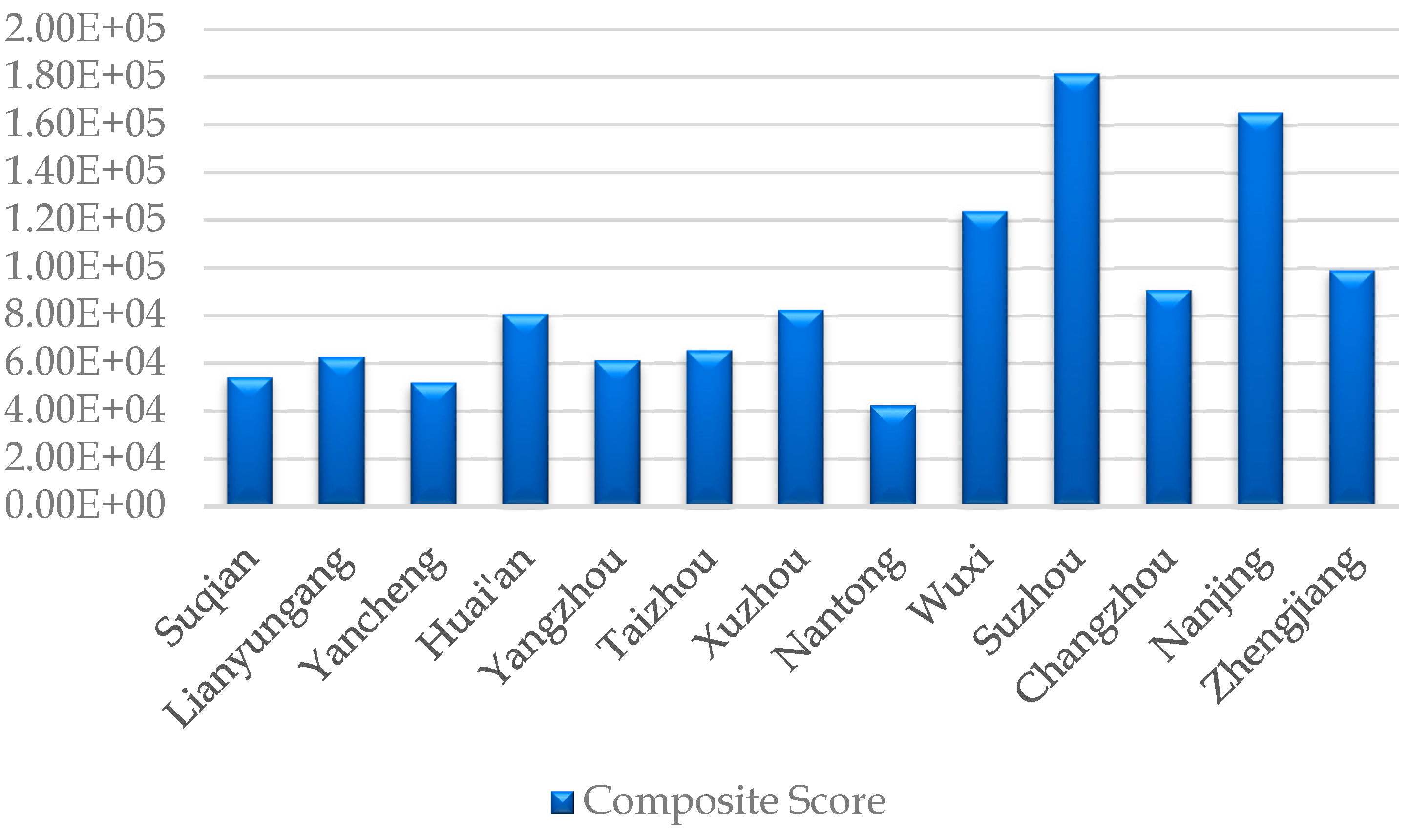
Correlation analysis was used to estimate the correlations between indicators and to determine the applicability of Principal Component Analysis. The Principal Component Analysis model transforms highly correlated variables into linearly uncorrelated variables through orthogonal transformations. By extracting the key information, the comprehensive scores for the ten indicators were obtained, among which the building area has the most significant impact on residential building carbon emissions, with a score of 0.136. Suzhou City in Jiangsu Province has the highest comprehensive score of 1.61568, indicating that Suzhou has the highest carbon emissions from the building process, followed by Nanjing, Wuxi, and Zhenjiang. Yancheng has the lowest carbon emissions from the building process, followed by Suqian and Yangzhou.

3.

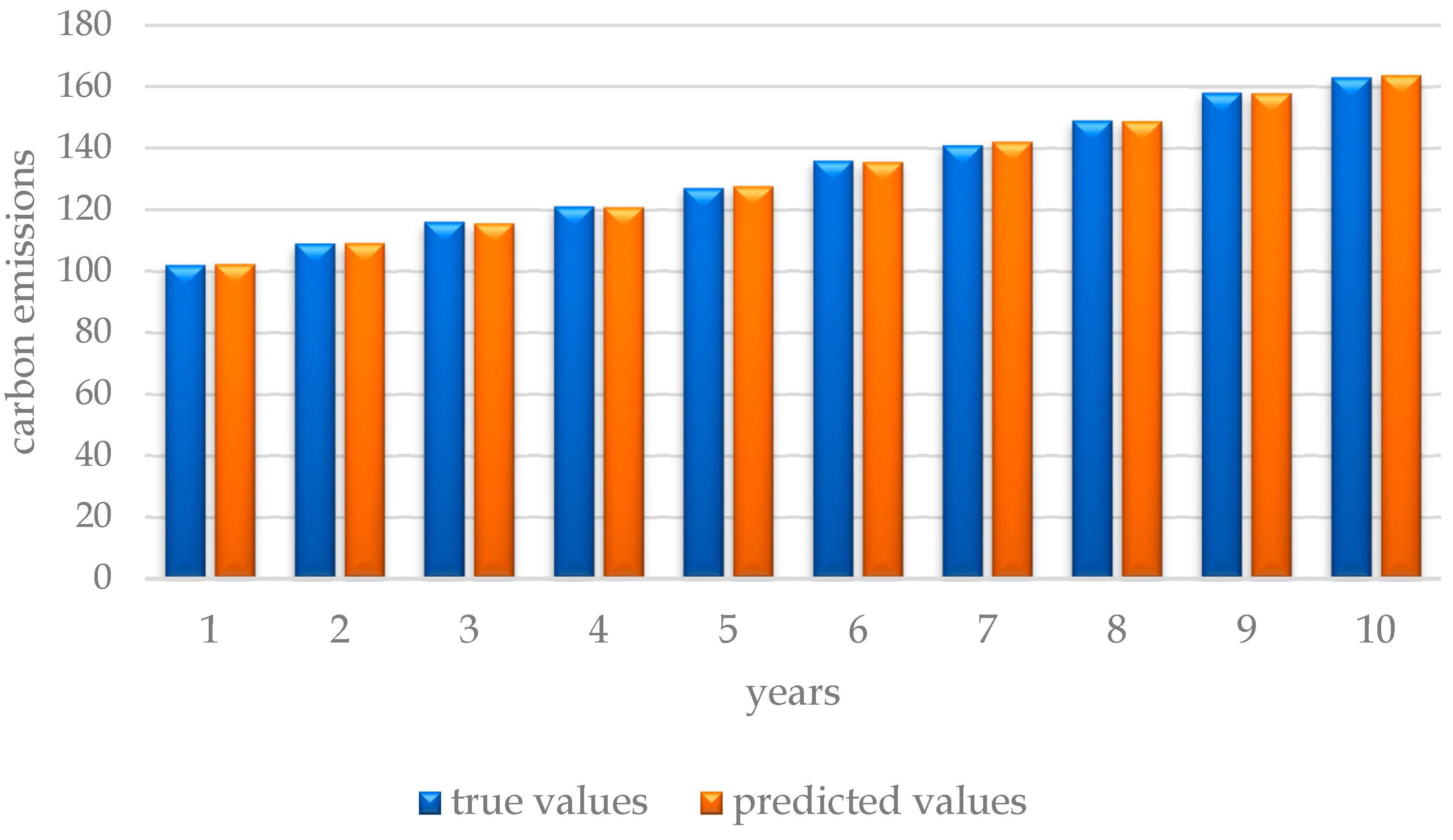
This paper introduced a grey prediction method for carbon emissions throughout the construction process, which is effective in the presence of uncertain information. The carbon emissions for 2024 are predicted using the GM(1,1) model within the grey prediction method, based on historical data of building carbon emissions from 2016 to 2023. The forecasted total carbon emissions for buildings in Jiangsu Province in 2024 is estimated to be 1.5576 million tons. Considering variations in temperature, rainfall, building energy consumption, and industrial output among regions, the feasibility of proposals must be evaluated. Different materials exhibit significant differences in thermal conductivity, thus affecting building insulation. Since energy consumption is higher in winter, prioritizing materials with better insulation could help reduce heating energy usage. Factors such as building area and energy consumption significantly impact carbon emissions, necessitating efficient building design and resource management.

4.

Significant disparities in carbon emissions exist among cities in Jiangsu Province, with southern cities emitting more than northern ones. Economic development plans should promote balance between regions, fostering green development to maintain equilibrium. Without intervention, residential building emissions are projected to double by 2031, highlighting the need for stringent control measures. By comprehensively utilizing these models and methods, decision-makers can better understand problems and enhance the accuracy and reliability of decisions.

5.

This study explores effective strategies for low-carbon building development and carbon emission control in Jiangsu Province. Through a detailed analysis of carbon emissions at each stage of a residential building’s life cycle (construction, operation, and demolition), the findings show that the building’s energy consumption and carbon emissions during the operational phase account for the largest portion of total emissions. Optimizing the selection of building materials, improving construction technology, and promoting energy-saving equipment and technologies are key measures to reduce carbon emissions throughout the life cycle of buildings. In addition, the mathematical model and evaluation method proposed in this paper provide a feasible reference framework for other regions and countries, which can help promote the development of low-carbon buildings worldwide. At the same time, it was found that the energy consumption and carbon emissions in the operation phase were significantly higher than those in the construction and demolition phases, mainly focusing on the use of indoor temperature regulation (such as air conditioning systems). By using energy-efficient building materials, improving construction techniques, and promoting intelligent control systems, a building’s total carbon emissions can be significantly reduced. Therefore, we recommend that the government and relevant departments formulate and promote building energy efficiency standards, strengthen support for the research and application of green building technologies, and provide corresponding incentives.

References

- Qu, J.; Guan, S.; Qin, J.; Zhang, W.; Li, Y.; Zhang, T. Estimates of cooling effect and energy savings for a cool white coating used on the roof of scale model buildings. Mater. Sci. Eng. 2019, 479, 012024. [Google Scholar] [CrossRef]
- Valdiserri, P.; Ballerini, V.; di Schio, E.R. Interpolating functions for CO2 emission factors in dynamic simulations: The special case of a heat pump. Sustain. Energy Technol. Assess. 2022, 53, 102725. [Google Scholar] [CrossRef]
- Shen, W.; Cao, L.; Li, Q.; Zhang, W.; Li, C. Quantifying CO2 emissions from China’s cement industry. Renew. Sustain. Energy Rev. 2015, 50, 1004–1012. [Google Scholar] [CrossRef]
- Institute for Climate Change and Sustainable Development, Tsinghua University. Research on China’s Long-Term Low-Carbon Development Strategy and Transformation Pathways; Environmental Publishing House: Beijing, China, 2021; pp. 220–260. (In Chinese) [Google Scholar]
- Li, Q.; Chen, Z.; Zhang, J.; Li, X.; Zhang, X. Insights from the Future Version of China’s CCUS Technology Roadmap (Update): An Analysis Based on the Perspective of the Global CCS Roadmap. Low Carbon World 2014, 7, 7–8. [Google Scholar]
- Li, Y.; Zhang, K.; Li, J. Comparative Analysis of Carbon Emissions in the Whole Life Cycle of Residential Buildings and Carbon Reduction Strategies. J. Xi’an Univ. Archit. Technol 2021, 53, 737–745. [Google Scholar] [CrossRef]
- Huang, Z.; Zhou, H.; Miao, Z.; Tang, H.; Lin, B.; Zhuang, W. Life-cycle Carbon Emissions in the Whole Life Cycle of Buildings: Connotation, Calculation, and Reduction. Engineering 2024, 35, 115–139. [Google Scholar] [CrossRef]
- China Construction Certification Center Co., Ltd.; Zhongtan Digital Laboratory. Research Report on Carbon Peak and Carbon Neutrality in China’s Construction Industry. 2022. Available online: http://www.jccchina.com/UserFiles/upload/file/20230324/20230324093145556.pdf (accessed on 19 July 2024). (In Chinese).
- China Association of Building Energy Efficiency. 2021 China Building Energy Consumption and Carbon Emission Research Report. 2021. Available online: https://mp.weixin.qq.com/s?__biz=MzIxODcxNDEwOQ==&mid=2247484041&idx=1&sn=0d6a67b96130de524e69d14ec76502a7&chksm=97e7181ba090910d71fc1d49d57ea7b2181c4537cf1689875aa8eb19a52b96e0eed56906d7c2&scene=27 (accessed on 19 July 2024). (In Chinese).
- Jiangsu Provincial Bureau of Statistics; Jiangsu Survey Office of the National Bureau of Statistics. 2023 Jiangsu Province National Economic and Social Development Statistical Bulletin. 2023. Available online: http://tj.jiangsu.gov.cn/art/2024/3/5/art_87595_11165526.html (accessed on 19 July 2024). (In Chinese)
- Xiao, Y.; Dai, R.; Zhang, G.; Chen, W. The Use of an Improved LSSVM and Joint Normalization on Temperature Prediction of Gearbox Output Shaft in DFWT. Energies 2017, 10, 1877. [Google Scholar] [CrossRef]
- Taherahmadi, J.; Noorollahi, Y.; Panahi, M. Toward comprehensive zero energy building definitions: A literature review and recommendations. Int. J. Sustain. Energy 2021, 40, 120–148. [Google Scholar] [CrossRef]
- Lu, C.; Wang, D.; Meng, P.; Yang, J.; Pang, M.; Wang, L. Research on Resource Curse Effect of Resource-Dependent Cities: Case Study of Qingyang, Jinchang and Baiyin in China. Sustainability 2019, 11, 91. [Google Scholar] [CrossRef]
- Likos, W.J. Modeling Thermal Conductivity Dryout Curves from Soil-Water Characteristic Curves. J. Geotech. Geoenviron. Eng. 2014, 140, 04013056. [Google Scholar] [CrossRef]
- Xing, W.; Ullmann, A.; Brauner, N.; Plawsky, J.; Peles, Y. Advancing micro-scale cooling by utilizing liquid-liquid phase separation. Sci. Rep. 2018, 8, 12093. [Google Scholar] [CrossRef] [PubMed]
- Luo, Z.; Cang, Y.; Zhang, N.; Yang, L.; Liu, J. A Quantitative Process-Based Inventory Study on Material Embodied Carbon Emissions of Residential, Office, and Commercial Buildings in China. J. Therm. Sci. 2019, 28, 1236–1251. [Google Scholar] [CrossRef]
- Banti, D.C.; Tsangas, M.; Samaras, P.; Zorpas, A. LCA of a Membrane Bioreactor Compared to Activated Sludge System for Municipal Wastewater Treatment. Membranes 2020, 10, 421. [Google Scholar] [CrossRef] [PubMed]
- Kaewunruen, S.; Sresakoolchai, J.; Peng, J. Life Cycle Cost, Energy and Carbon Assessments of Beijing-Shanghai High-Speed Railway. Sustainability 2020, 12, 206. [Google Scholar] [CrossRef]
- Zou, Y.; He, Y.; Lin, W.; Fang, S. China’s regional public safety efficiency: A data envelopment analysis approach. Ann. Reg. Sci. 2021, 66, 409–438. [Google Scholar] [CrossRef]
- Sun, L.; Yu, S.; Ji, Y.; Zhou, P.; He, Y.; Weerasinghe, R. Air Environment Pollution and Management Measures at Bulk Terminals. E3S Web Conf. 2020, 143, 02037. [Google Scholar] [CrossRef]
- Binarti, F.; Koerniawan, M.D.; Triyadi, S.; Utami, S.S. Maximizing the ENVI-met Capability of Modelling the Mean Radiant Temperature of a Tropical Archaeological Site. IOP Conf. Ser. Earth Environ. Sci. 2020, 541, 012005. [Google Scholar] [CrossRef]
- Zhang, R.; Zhang, R.; Gao, H.; Zhang, Y. The New Design of Syrup Drug Delivery Device. IOP Conf. Ser. Earth Environ. Sci. 2019, 358, 032004. [Google Scholar] [CrossRef]
- Ibrahim, F.H.; Yusoff, F.M.; Fitrianto, A.; Nuruddin, A.A.; Gandaseca, S.; Samdin, Z.; Kamarudin, N.; Nurhidayu, S.; Kassim, M.R.; Hakeem, K.R.; et al. How to develop a comprehensive Mangrove Quality Index? MethodsX 2019, 6, 1591–1599. [Google Scholar] [CrossRef]
- Johnsson, M.; Henriksen, R.; Fogelholm, J.; Höglund, A.; Jensen, P.; Wright, D. Genetics and Genomics of Social Behavior in a Chicken Model. Genetics 2018, 209, 209–221. [Google Scholar] [CrossRef]
- Zheng, H.; Xia, X.; Gu, J.; Xia, Y.; Li, M.; Zhao, L.; Jin, X. Current Status, Transformation, and Countermeasures of Social Development Under the Goals of ‘Peak Carbon’ and ‘Carbon Neutrality’. Ind. Metrol. 2024, 33, 55–60+79. [Google Scholar] [CrossRef]
- Li, J.; Liu, Y. Calculation Model of Carbon Emissions from Construction Projects Based on Whole Life Cycle. J. Eng. Manag. 2015, 29, 12–16. [Google Scholar] [CrossRef]
- Qi, X.; Shi, L.; Crockforce, K.; Zhou, M. Comparison Study on Calculation and Environmental Impact of Residential Building Lifecycle Carbon Emissions Between China and Finland. World Archit. 2024, 1, 104–109. [Google Scholar]
- Cao, Q. Research on Multispectral Dimensionality Reduction Algorithm Based on Second Order Polynomial Regression and Weighted Principal Component Analysis. Opt. Tech. 2024, 49, 250–256. [Google Scholar] [CrossRef]
- Gou, X.; Mi, C.; Zeng, B.; Li, M.; Xu, Y. New Seasonal Discrete Grey Prediction Model and Its Application from Longitudinal and Horizontal Dimensions Perspective. Chin. J. Manag. Sci. 2024, 1–12. [Google Scholar] [CrossRef]
- Ma, Q.; Li, S.; Ding, B.; Hou, M. Analysis of Precision Inspection Items of CNC Turning and Milling Compound Machine Tool. Met. Process. Cold Work. 2024, 4, 61–64. [Google Scholar]
- Zhang, S.; Wang, K. Research on Control Indicators of Carbon Emissions for Low-Carbon, Near-Zero Carbon, and Zero Carbon Residential Buildings. Build. Sci. 2024, 39, 11–19+57. [Google Scholar]
- Hu, J.; Wang, Z.; Pan, Y.; Li, P. Research on Thermal Conduction Model of Regenerative Cooling U-shaped Channel in Supercharged Pulse Detonation Engine. Propuls. Technol. 2022, 43, 152–163. [Google Scholar] [CrossRef]
- Li, Z.; Wu, X.; Yuan, T.; Mao, W. Numerical Analysis Model of Circuit Breaker Short-Circuit Closing Process and Its Application in Arcing Fault Selection. High Volt. Appar. 2022, 58, 180–187. [Google Scholar] [CrossRef]
- Sun, J.; Xin, Y.; Zhang, C.X.; Zhao, Y.; Wang, Z.F. Application of Principal Component Analysis Method in Water Quality Evaluation of Yubiao Reservoir. Tianjin Agric. For. Sci. Technol. 2024, 2, 10–12. [Google Scholar] [CrossRef]
- Li, W. Quantifying the Building Energy Dynamics of Manhattan, New York City, Using an Urban Building Energy Model and Localized Weather Data. Energies 2020, 13, 3244. [Google Scholar] [CrossRef]