Abstract
Lithium ion (Li-ion) battery packs have become the most popular option for powering electric vehicles (EVs). However, they have certain drawbacks, such as high temperatures and potential safety concerns as a result of chemical reactions that occur during their charging and discharging processes. These can cause thermal runaway and sudden deterioration, and therefore, efficient thermal management systems are essential to boost battery life span and overall performance. An electrochemical-thermal (ECT) model for Li-ion batteries and a conjugate heat transfer model for three-dimensional (3D) fluid flow and heat transfer are developed using COMSOL Multiphysics®. These are used within a novel computational fluid dynamics (CFD)-enabled multi-objective optimization approach, which is used to explore the effect of the mini-channel cold plates’ geometrical parameters on key performance metrics (battery maximum temperature (), pressure drop (), and temperature standard deviation ()). The performance of two machine learning (ML) surrogate methods, radial basis functions (RBFs) and Gaussian process (GP), is compared. The results indicate that the GP ML approach is the most effective. Global minima for the maximum temperature, temperature standard deviation, and pressure drop (, , and , respectively) are identified using single objective optimization. The third version of the generalized differential evaluation (GDE3) algorithm is then used along with the GP surrogate models to perform multi-objective design optimization (MODO). Pareto fronts are generated to demonstrate the potential trade-offs between , , and . The obtained optimization results show that the maximum temperature dropped from 36.38 to 35.98 °C, the pressure drop dramatically decreased from 782.82 to 487.16 Pa, and the temperature standard deviation decreased from 2.14 to 2.12 K; the corresponding optimum design parameters are the channel width of 8 mm and the horizontal spacing near the cold plate margin of 5 mm.
1. Introduction
The worldwide use of internal combustion engine vehicles has resulted in a number of environmental problems, including greenhouse gas (GHG) emissions, significant air quality degradation, and negative health effects on humans [1]. Therefore, the automobile industry is currently shifting towards more environmentally friendly and sustainable vehicles. Electric vehicles (EVs), specifically battery electric vehicles (BEVs) powered by low-emission electricity, can significantly decrease GHG emissions and improve air quality [2].
The majority of batteries used in modern EVs are lithium-ion (Li-ion) ones, which dominate other battery types, including lead-acid, lithium–sulfur (Li-S), and nickel metal hydroxide (Ni-MH), due to their higher energy density [3], longer life cycles [4], lower self-discharge rates [5], and greater environmental friendliness [6]. However, a major problem with Li-ion batteries is that they generate a significant amount of heat that can cause temperatures above the acceptable operating range [7], which can lead to reduced battery life, performance degradation, and safety concerns due to thermal runaway [8]. Furthermore, it is generally agreed that there should be a maximum temperature variation of less than 5 °C between the cells inside the battery module [8]. Consequently, effective battery thermal management systems (BTMSs) are needed to keep them running safely and effectively.
Recently, thermal management has received significant attention across several distinct fields, including electronics [9], buildings [10], EVs [11], data centers [12], aerospace [13], medical devices [14], fuel cells [15], etc. For EVs, several types of BTMSs have been considered, including air cooling systems [16], phase change materials (PCMs) [17], single- and multi-phase liquid cooling systems [18,19], and hybrids of these [20,21]. Due to their higher efficiency and cooling capacity, liquid-cooled BTMSs dominate the current EV market for power battery packs and powertrain systems [18], and, due to the limited available space in EV batteries, cold plates are generally preferred [22]. Since they rely on indirect contact cooling, they provide better separation between the battery module and its surroundings, leading to safer operation [23]. As a result of the micro-channels’ high power density dissipation capacity—up to [24]—and their effectiveness in managing heat fluxes, which range from a few to several [25,26], cold plates-based mini-channels are a promising approach for cooling EV Li-ion batteries within this range.
A number of recent studies have focused on optimizing the mini-channel configurations in cold plates using computational fluid dynamics-enabled surrogate modeling. Li et al. [27], for example, optimized parallel mini-channel cold plate geometries and achieved reductions in the maximum temperature difference, temperature standard deviation, and pressure drop of 5.7%, 0.82%, and 44.5%, respectively. More recent studies by Wang et al. [28] optimized a serpentine microchannel cold plate geometry, while Zhang et al. [29] optimized the channel design parameters for 24 liquid-cooled plate channel configurations. More complex channel configurations have also been considered. Li et al. [30], for example, optimized a diamond-type flow channel with six design parameters, while Dong et al. [31] optimized a cold plate with bionic lotus leaf channels and design variables such as channel spacing, channel width, channel angle, and mass flow rate. Liu et al. [32] optimized a bionic leaf vein branch (BLVB) channel cold plate. Wu et al. [33] optimized BTMS based on a variable heat transfer path cooling plate and achieved a reduction of temperature difference across the battery surface while slightly increasing the maximum temperature on the battery surface. Feng et al. [34] optimized a unique gradient distributed Tesla cold plate and achieved a significant reduction in pressure drop by 75.7% in Pareto frontier solution compared to the cells’ maximum temperature difference that varied within a small range (11.2–12.6 °C). Sui et al. [35] optimized a cold plate equipped with hybrid manifold channels and design variables including parallel channel width, manifold channel width, parallel channel height, and the inlet velocity.
Clearly, accurate modeling of the heat generation with Li-ion batteries is essential for creating high fidelity heat transfer models in Li-ion BTMSs. Most previous studies either make the physically unrealistic assumption that the heat generation rate is steady [36] or use empirical relationships based on a limited series of experiments. Time-dependent heat generation rate models are preferable, and a number of these have also been proposed, including the Newman, Tiedemann, Gu, and Kim (NTGK) model [37], the equivalent circuit model (ECM) [38,39,40], and the Newman pseudo two-dimensional (P2D) model [41]. The latter is widely used for physics-based electrochemical-thermal ECT modeling and accounts for the mobility of lithium ions within the solid electrode particles and the reaction kinetics at the electrode/electrolyte interfaces [42]. The present study discusses the challenges of validating the P2D model and in particular its reliance on numerous physical parameters whose values are uncertain or that have widely ranging values in the literature. Following validation, the P2D model is used for the first time within a novel CFD-enabled optimization methodology for mini-channel cold plates (MCCPs) of Li-ion BTMS to explore trade-offs between temperature standard deviation, pressure drop, and maximum temperature.
The paper is organized as follows. Section 2 describes the numerical simulation methodology that covers the physical problem, the electrochemical, coupled electrochemical-thermal battery, and conjugate heat transfer models along with their associated governing equations, modeling parameters, and boundary conditions. Section 3 presents a comprehensive validation and verification of the numerical methods and the mesh sensitivity studies. The surrogate-enabled optimization methodologies are described in Section 4. Section 5 presents a comprehensive set of optimization results and optimized designs. Conclusions are drawn in Section 6.
2. Numerical Simulation Methodology
2.1. Physical Problem
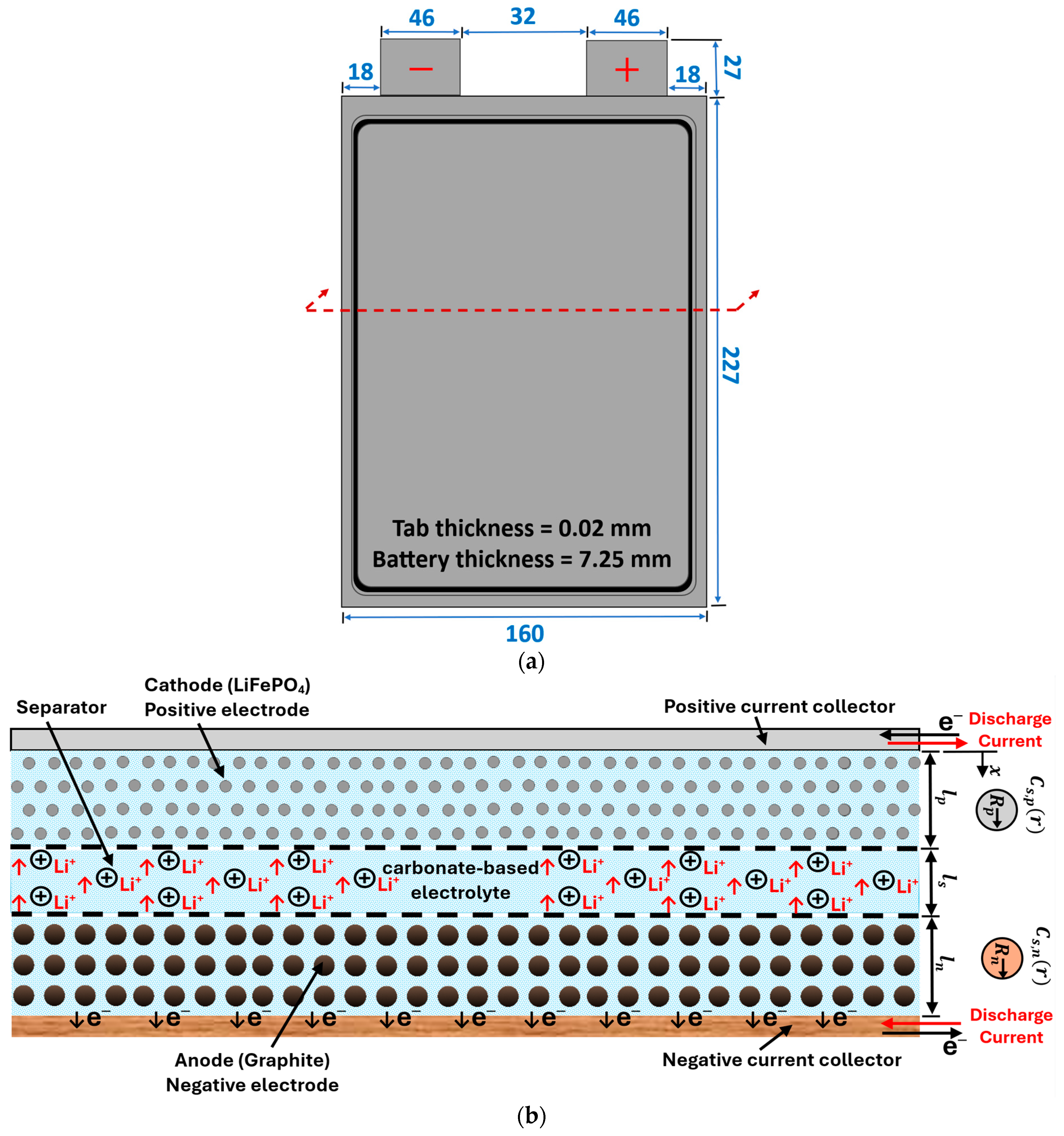
The basic components of the 20 Ah and 3.3 V prismatic pouch cell investigated in the present work are graphite for the anode, lithium iron phosphate (LiFePO4) for the cathode, and a carbonate-based electrolyte. The cell specifications are given in Table 1 [43].

Table 1.
The specifications of the 20 Ah LiFePO4 pouch cell [43].
Figure 1a shows a schematic diagram of a single unit cell along with the dimensions. The corresponding cross-sectional view of this cell is shown in Figure 1b. When a Li-ion battery cell is being charged and discharged, lithium ions are extracted and inserted into the solid particles of the positive and negative porous electrodes. They migrate between the positive and negative electrodes, as well as the separator region, due to a concentration gradient [44]. Many physical and chemical processes are involved, including the diffusion of Li ions (intercalation and de-intercalation) within active solid electrode particles, electrochemical reactions at the solid–electrolyte interfaces, diffusion of Li ions in the liquid electrolytes, and the generation of heat during the battery operation. In the current work, five of the aforementioned pouch battery cells are arranged in a series to create a battery module. As shown in Figure 2, the battery cells are cooled by using aluminum cold plates, which are composed of parallel straight minichannels organized in a manner where each cold plate is placed between two consecutive cells. Figure 2 also displays the geometrical details of the cold plate half domain and the simulated battery module, where the symmetry is exploited to reduce the computational time.
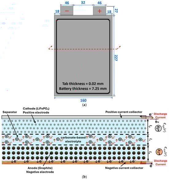
Figure 1.
(a) Schematic diagram of a single unit cell (units: mm); (b) the unit cell cross-sectional view.
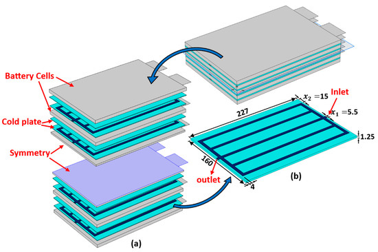
Figure 2.
The proposed schematics of the BTMS: (a) internal configuration of the battery module; (b) half of the domain of a single minichannel cold plate (units: mm).
2.2. Numerical Analysis of the Electro-Chemical Model
Due to the importance of accounting accurately for the time-dependent electro-chemical heat generation with the battery module, the pseudo two-dimensional electro-chemical thermal (P2D-ECT) model is used. This is based on the Newman electrochemical (EC) model and has been shown to be successful in simulating cell performance [45]. The model has two dimensions, x and r. The x value represents the dimension along the cell thickness direction, which encompasses the thicknesses of the negative electrode, separator, and positive electrode. It mimics mass and charge transfer within the solid-phase electrodes, liquid electrolytes, and the charge-transferring reaction at the electrode-electrolyte interface. The value r is related to the radius of solid-phase particles. This is used for solving diffusion equations using spherical coordinates within the solid-phase particles. The main assumptions of the P2D-ECT model are summarized in Table 2.
Table 2.
The main assumptions of this P2D-EC model.
The main governing equations for mass and charge conservations in both solid and liquid-electrolyte phases and the Butler–Volmer equation, along with their corresponding boundary conditions, are described below.
2.2.1. Governing Equations in the Porous Electrodes (Anode and Cathode)
The governing equations for positive and negative porous electrodes can be represented by mass and charge conservation in the solid phase, mass and charge conservation in the liquid electrolyte, and electrochemical reactions that take place at the solid–electrolyte interface–the Butler–Volmer equation. This complex coupled system of equations is described next.
- Mass and charge conservation in the solid phase:
Fick’s second law in a spherical coordinate system describes the mass balance of Li-ions in an intercalation particle of electrode active material as follows [49]:
For constant charge/discharge current, the boundary conditions of Equation (1) are as follows [50]:
where indicates whether the equation is solved for the positive or negative porous electrode. is the solid phase diffusion coefficient (), and is the Li-ion concentration in the intercalation particle (). refers to the radial coordinate along the intercalation particle (). refers to the intercalation particle’s radius (). is the molar flux of lithium ions at the surface (.
Charge conservation in the solid phase of the electrode region is governed by the generalized Ohm’s law [46]:
where is the current density in the solid phase of the electrode () and is the solid phase potential (V). is the electrical conductivity of the solid phase in the electrode (). This value can be corrected to the effective value for both positive and negative electrodes and can generally be expressed as follows [51]:
where , are the volume fractions of the solid phase active material in the positive and negative electrodes, respectively. The fundamental relation between the mass flux of Li ions and the solid phase current is given by Faraday’s law [46]:
where is the Faraday constant (). is the solid–electrolyte interfacial area per unit volume () and is given by [52]:
Integrating Faraday’s and Ohm’s laws establishes a link between the solid phase potential in the electrode and the rate of reaction [46]:
As the current enters the battery cell at and leaves at , the boundary conditions are as follows:
, the total current passing through the cell, is positive for the charge process and negative for the discharge process (A). is the applied current density of the battery (), and A is the electrode plate area (). , , and represent the lengths of the positive electrodes, negative electrodes, and separator, respectively (. An alternate boundary condition for the solid potential is as follows:
At the electrodes–separator interface ( and ), charge transport occurs through the liquid electrolyte. Thus, the solid phase current is zero at these interfaces:
- Mass and charge conservation in the electrolyte (liquid phase):
Mass conservation in the electrolyte is described by [46] as follows:
Because Li ions do not enter or exit the cell, the boundary condition for the Li-ion mass conservation equation is zero mass flux at the boundaries of the current collector [46]:
where refers to the volume fraction of the electrolyte phase in the electrode (note: , where is the volume fraction of the filler material in the electrode). is the electrolyte’s Li-ion concentration (, and is the electrolyte’s Li-ion transport number. is the current density in the electrolyte (. is the effective diffusivity of the electrolyte () and is obtained via the following:
where is the diffusivity of the electrolyte (), and is the Bruggeman porosity exponent. Charge conservation in the electrolyte is governed by the concentrated solution theory and is expressed as follows [46]:
The insulation boundary conditions are set at the cell’s two ends ( and ), indicating that current enters and exits the cell through solid particles in contact with current collectors [46]:
where is the electrolyte phase potential (). is the universal gas constant (). is the temperature (). is the activity dependence of the electrolyte. is the effective electrolyte electrical conductivity in the porous electrode () and is given by the following:
where is the electrolyte electrical conductivity ().
The following equations are also needed to model charge and mass conservation in a porous electrode [53,54]:
where represents local current density at the particle surface (.
- Electrochemical reactions at the solid–electrolyte interface:
The rate of the electrochemical reactions on the surface of the solid electrode particles is generally governed by the Butler–Volmer equation, which combines both charge-mass conservation equations and is written as follows [48]:
where is the exchange current density ( and is given by the following [43]:
and are transfer coefficients for the anode and cathode, respectively. is the reference exchange current density (. is the electrolyte reference concentration (). refers to the maximum Li-ions concentration in the intercalation particles (), and is the Li concentration at the surface of the intercalation particles (). is the local surface overpotential () and is expressed as follows [55,56]:
where is the voltage drop across the film resistance (), and represents the film resistance (). is the open-circuit potential (equilibrium potential) (), which is dependent on the temperature (T) and state of charge (SOC) of the electrodes. It is expressed as follows:
where is the reference temperature and is the open circuit potential under the reference temperature .
2.2.2. Governing Equations in the Liquid Electrolyte (Separator)
The conservation equations for mass and charge in the separator, when only the electrolyte is present, approximately match with similar equations governing electrolyte behavior in the porous electrode. Because there is no reaction in the separator zone, Equation (13) simply becomes as follows [46]:
Since all current passes through the separator zone, Equation (16) has the following form in the separator [46]:
The acronym , which appears in the two equations above along with physical parameters, refers to the separator zone.
2.3. Numerical Analysis of the Coupled Electrochemical-Thermal Battery Model
A three-dimensional (3D) coupled electrochemical-thermal (ECT) model of the Li-ion battery cell is developed using COMSOL Multiphysics 6.0. The electrochemical model is used to calculate the average heat generation rate () during the electrochemical reactions, which is an essential input for the thermal model. At the same time, the average temperature () that is obtained from the thermal model acts as the initial condition for the electrochemical model, constructing an iterative solution procedure that takes into consideration the impact of temperature changes on the electrochemical reactions.
The general energy conservation equation for a single battery cell is given by the following:
where , , and are the thermal conductivity, density, and specific heat of the battery cell, respectively. is the convective heat transfer from the surfaces surrounded by the ambient air given by Newton’s law of cooling:
where , , , and are the convective heat transfer coefficient, area of battery surfaces exposed to the air, battery surface temperature exposed to air, and ambient temperature, respectively. represents the total heat generation rate per unit volume of the battery and can be written as follows:
where , , , and are the heat generation rates at the positive electrode, negative electrode, separator, and current collectors, respectively (). Each of the two variables, and , has three heat generation terms: reversible heat generation (), polarization heat generation (), and ohmic heat generation (). The latter two terms are referred to as the irreversible heat generation (). The equations for each of these terms are given by the following [57,58]:
It is assumed that the contribution from the film resistance resistive heating term is not included in the polarization heat generation rate. The heat generation from the positive and negative current collectors will be identified in the positive and negative tabs and can be further represented by the following [43]:
where is the electrical conductivity for the positive and negative current collectors. is the gain term used to express the compensation for the tabs’ junction resistance (, where the junction resistance is the main source of heat in the tabs. is the resistivity of the positive and negative tab, (). The resistivity expressions and temperature dependency parameters used in the current study are given in Table 3 based on the various temperature ranges.
Table 3.
Resistivity expressions based on the various temperature ranges [43].
Finding the correct set of battery parameters is one of the main challenges with battery modeling because manufacturers usually do not reveal these details in their specification sheets, and determining these parameters is a difficult and time-consuming process that calls for a variety of characterization and analytical methods [42]. As a common procedure within the battery modeling community, parameter sets are usually sourced from literature, albeit their sources are not always known [59]. The material properties and electrochemical and thermal parameters of the Li-ion battery cells used in the numerical simulations are listed in Table 4. Since some of the parameters needed to specify the problem are missing in the literature, these have been obtained through private communication with Mevawalla et al. [43]; the rest were obtained from their original publication. The applied current density for the P2D model, , can be calculated by knowing the electrode plate area [59,60,61]. However, in this work, the applied current density at high C-rate (4C) has been obtained via a private communication with Mevawalla et al. [43].
Table 4.
Li-ion battery parameters [43].
2.4. Conjugate Heat Transfer Modeling
A three-dimensional (3D) conjugate heat transfer model that simulates heat conduction in the solid and convective heat transfer to the cooling fluid (water) and surrounding air is used to simulate the performance of the minichannel cold plate cooling system. The continuity and momentum equations of the water within the cold plate minichannels are given by the following:
where , , and are the density, viscosity, pressure, and velocity of the water, respectively. The energy conservation equations for the water and cold plate are given by the following:
where and are the heat capacity and temperature of the water, respectively. , , , and are the density, heat capacity, thermal conductivity, and temperature of the cold plate, respectively. Table 5 is a list of all relevant boundary conditions and assumptions used in the conjugate heat transfer model. The physical parameters and temperature dependency expressions for the cooling fluid (water), cold plate, and battery tab used in the current study are given in Table 6.
Table 5.
The boundary conditions of the conjugate heat transfer model.
Table 6.
The physical parameters for battery tab, cooling fluid, and cold plate, respectively.
In this paper, the performance of the BTMS is evaluated using important practical metrics [63], namely the maximum temperature of the battery cells (, the temperature standard deviation (, and the pressure drop of the water in the minichannels (. These are given, respectively, by the following:
where the and A are the average temperature and area of the battery cells, respectively. and are the inlet and outlet pressures of the water. After the battery cells have fully discharged, , , and values are calculated at the minimum voltage (stop voltage) of 2 V, the point at which heat generation peaks.
3. Numerical Validation and Verification
3.1. Conjugate Heat Transfer Modeling
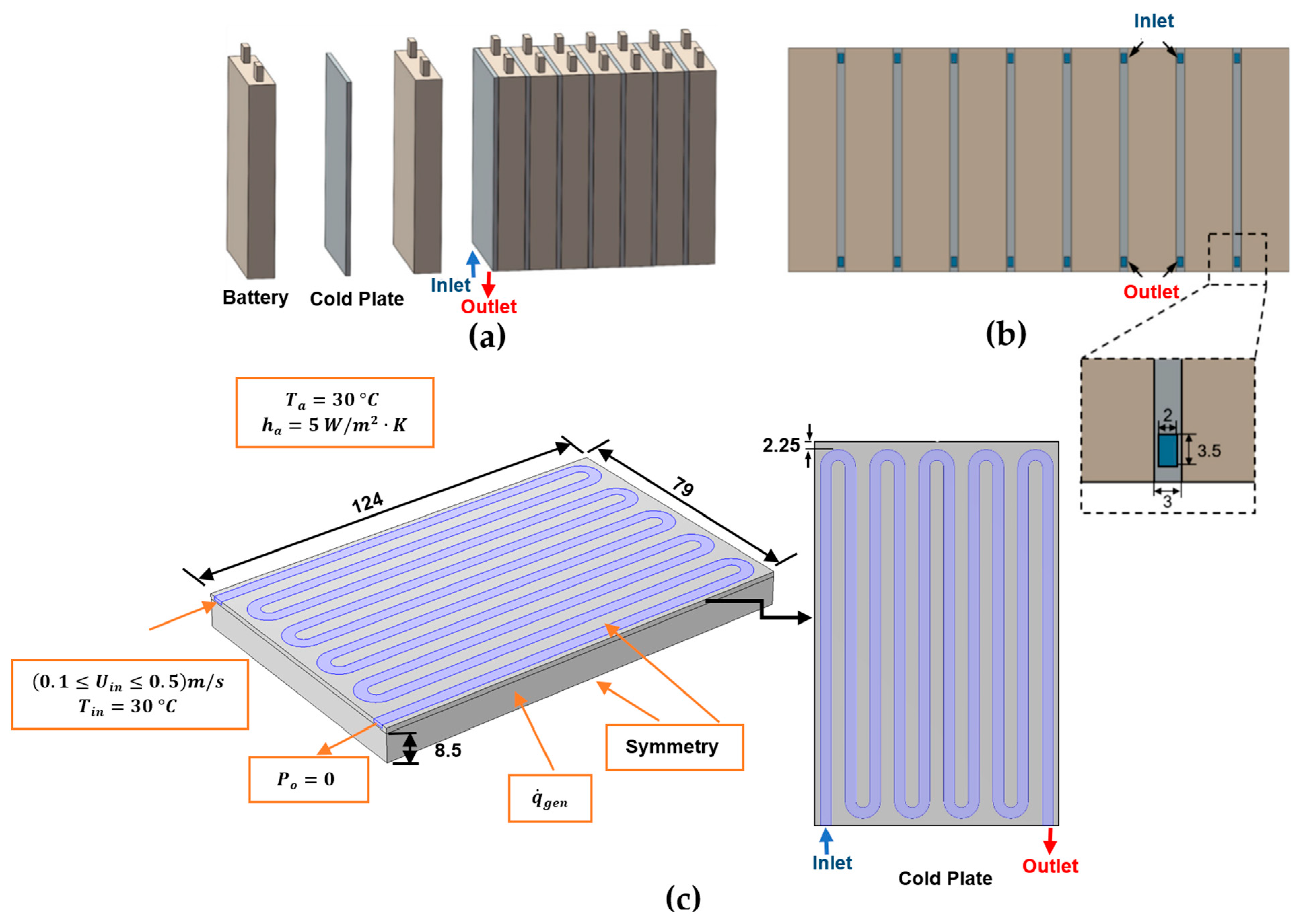
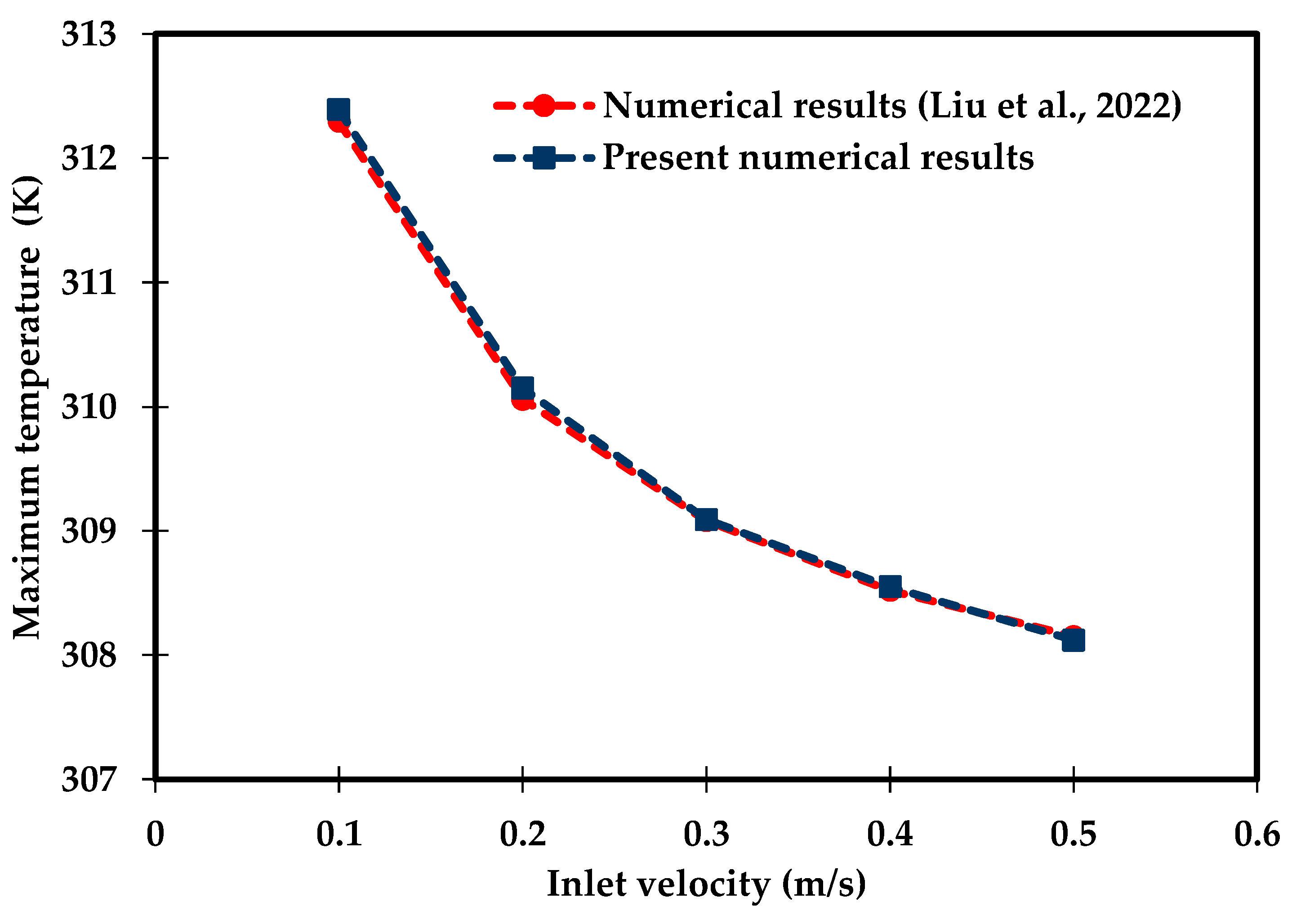
The first validation is against a recent numerical result obtained by Liu et al. [64] for the BTMS based on case 1 including 8.0 Ah prismatic LiFePO4 Li-ion batteries cooled by minichannel cold plates. This uses a much simpler empirical method for specifying the heat generation rate based on an empirical polynomial heat generation rate expression based on experiments for a 9 C discharge rate [65]. Their BTMS layout is shown in Figure 3. Figure 3a depicts the BTMS, where each cold plate is inserted between consecutive battery cells; Figure 3b shows the BTMS’s bottom view; and Figure 3c displays the configuration, boundary conditions, and geometrical parameters for half of the domain of a single battery unit and serpentine minichannel cold plate configuration, where symmetry has been exploited. The water inlet temperature and velocity range are set at 30 °C and (0.1 ≤ m/s, respectively. The polynomial heat generation rate fitting equation is given in Equation (47).
where the heat generation is estimated in (), and , the cell state of charge, is denoted by the following:
where I, C are the discharge current and nominal capacity of the battery, respectively, and t represents the discharge time.

Figure 3.
Schematics of the BTMS based on case 1 of Liu et al.’s [64] work using the polynomial heat generation method: (a) battery module; (b) bottom view; (c) half of the domain of a single battery unit and a serpentine minichannel cold plate (units: mm).
A CFD model of this configuration has been developed in COMSOL 6.0 using a free-tetrahedral mesh of (266,901) elements and time steps of 2 s. The results were evaluated in terms of the maximum battery temperature over the water inlet velocity range () . Figure 4 shows excellent agreement between the present model and the numerical results obtained by Liu et al. [64], with a mean absolute percentage error (MAPE) of 0.02. MAPE is computed using Equation (49):
where (N) is the number of evaluated points.

Figure 4.
Comparison of the numerical results obtained for the maximum battery temperature with Liu et al. [64].
The simulation of the BTMS based on an empirical polynomial heat generation rate takes around 32 minutes to complete on a Dell computer running Windows 10 with a 12th Gen Intel(R) Core (TM) i7-1270P 2.20 GHz processor and 32.0 GB of RAM.
3.2. P2D-ECT Modeling
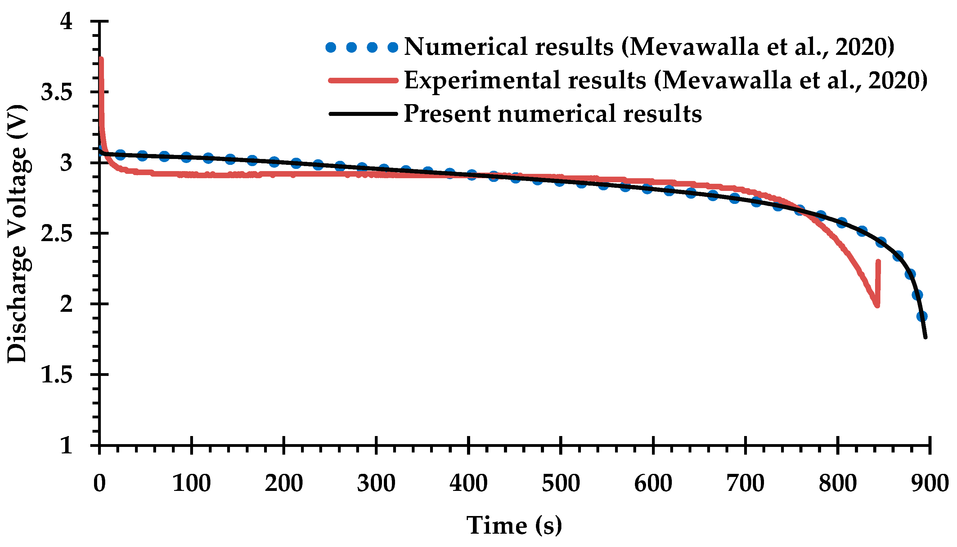
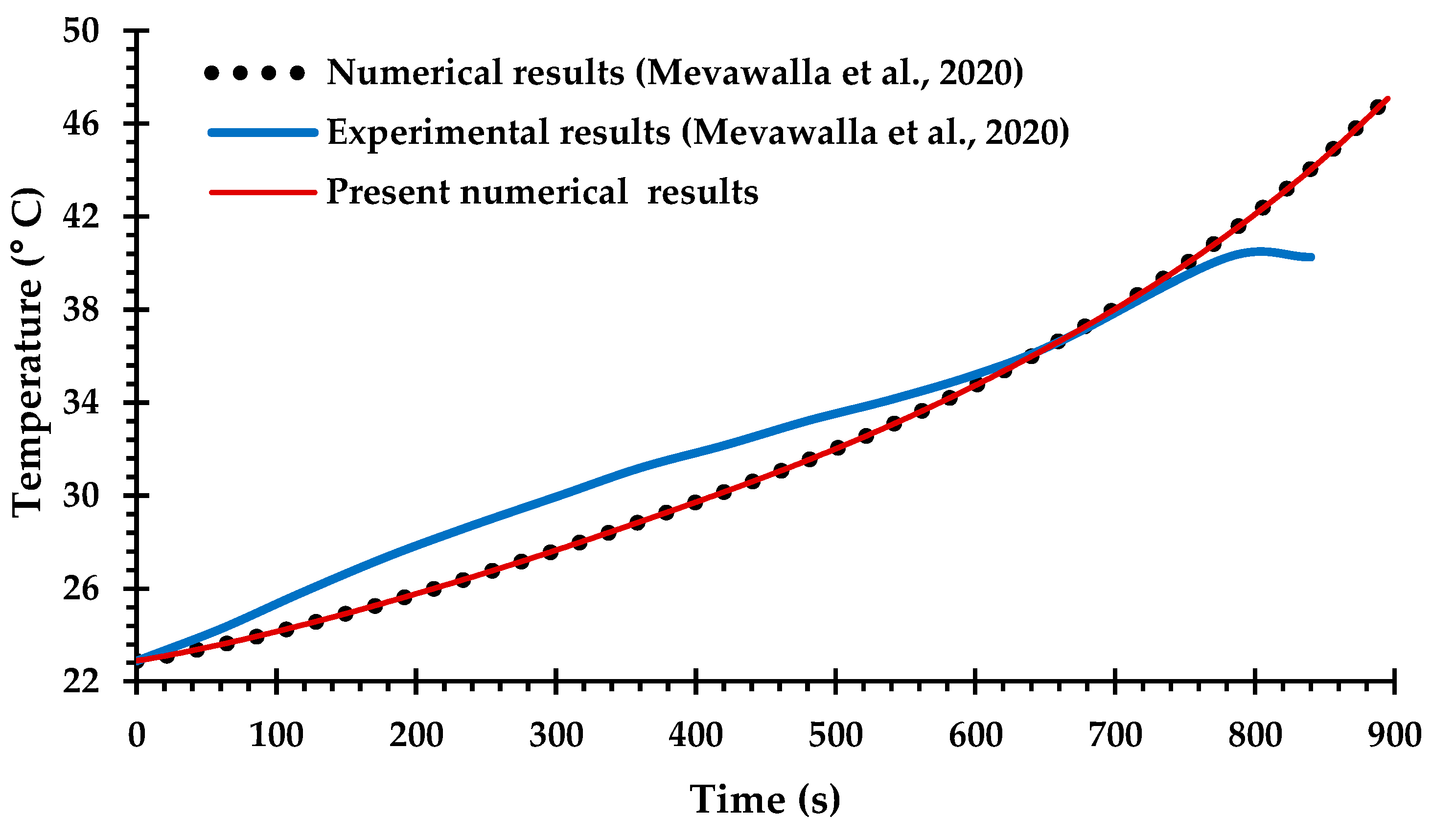
Only a small number of previous studies of BTMS have attempted Li-ion battery cooling with coupling between the electro-chemical heat generation processes and the MCCPs cooling system, due to difficulties in determining many of the key modeling parameters for commercial Li-ion batteries [42,66] and the computational challenges of solving the coupled equations. The experimental and numerical results obtained by Mevawalla et al. [43] are used here to validate the heat generation rate predicted by the present ECT model. Specifically, a single 20 Ah LiFePO4 Li-ion pouch battery cell without a cold plate is simulated at a high discharge rate of 4C using a free tetrahedral mesh of (10,032) elements. Comparisons are shown in Figure 5 and Figure 6 for the discharge voltage profile and the average surface temperature on both sides of the cell. Once again, there is generally good agreement with the results of Mevawalla et al. [43].
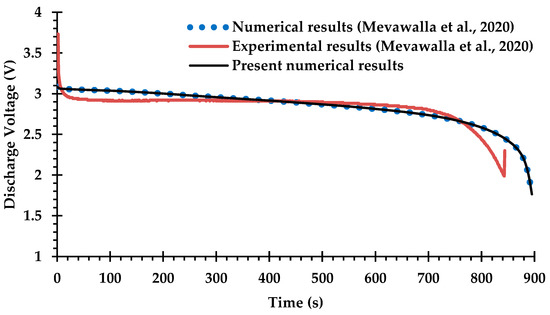
Figure 5.
Comparison of discharge voltage profiles between the present observations and the experimental and numerical observations of Mevawalla et al. [43].
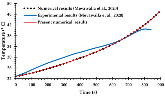
Figure 6.
Comparison of average battery surface temperature between the present observations and the experimental and numerical observations of Mevawalla et al. [43].
The effect of mesh density on the numerical solutions is now considered using unstructured free tetrahedral meshes. A constant mass flow rate of kg/s is applied in each minichannel, and the numerical results are obtained when the 20 Ah Li-ion battery cells are fully discharged at 4C and at a minimum stopping voltage of 2.0 V. The geometrical dimensions of the BTMS are shown in Figure 2, where a symmetry condition is used to reduce computational time. Results are given in Table 7, showing how the number of elements affects the maximum temperature in the Li-ion batteries and the pressure drop in the minichannel cold plates.
Table 7.
Grid sensitivity results.
The percentage relative error (PRE) of results on each mesh with respect to those on the finest mesh are calculated using Equation (50):
P is the numerical solution of the evaluated values of the physical parameters ( and ) for a given number of elements (i). The BTMS model with elements is used for the simulation presented below, as it offers an appropriate balance between computational time and simulation accuracy.
The coupled system of P2D-ECT and conjugate heat transfer model equations are solved using COMSOL Multiphysics 6.0 with a 5 s time step and a relative tolerance of 0.001. Each simulation takes around 15 h on the University of Leeds Advanced Research Computing (ARC4) HPC system.
4. Multi-Objective Design Optimization of Cold Plate Minichannels
The validated P2D-ECT model is used within a surrogate-enabled optimization strategy to explore and optimize the minichannel geometry within a cold plate cooling system. The key objectives to be minimized are the maximum temperature, , the standard deviation of the temperature, , and the pressure drop, . The design variables are the variables and in Figure 2, relating to the channel width and horizontal spacing near the margin of the cold plate, respectively, and take the limits and , respectively.
Optimal Latin hypercube sampling is used to generate 20 design of experiment (DoE) points within the design space at which the P2D-ECT model is run to compute , , and . The performances of two different surrogate modeling approaches are assessed. The first uses Gaussian radial basis functions (RBFs). The RBFs surrogate modeling approach is a very simple and effective approach [67,68] based on surrogate model approximations for each objective function at every design point, , in terms of the n DoE points () of the form [69]:
Note that these depend on a single hyper-parameter, , refers to objective functions (, , and ), and is the number of design of experiment points. The values are the RBF weights that ensure that the surrogate model is interpolative, so that at every DoE point for . Leave-one-out cross validation (LOOCV) is used to optimize the hyperparameter β with respect to the mean square error (MSE). The MSE metric is a widely used metric that represents the average squared difference between the predicted and actual values. It is given by the following:
where represents the number of observations, and , are the actual and predicted values for the objective function, respectively.
After the optimal value of has been determined, the vector of weights can be determined via the following:
The second approach uses Gaussian process (GP) regression, which is widely used in ML applications [70] due to its flexibility and ability to predict uncertainties. GP is a powerful and popular ML method that offers the potential to estimate errors on a sound mathematical basis. It also works well for surrogate modeling of small datasets [71,72,73]. The GP model is comprised of two terms: the mean and a random variable called , which represents variance [74]:
The correlation matrix is given by the RBF kernel, a function of the distance between their corresponding points in a sampling plan ( and ) [75]:
where represents the number of the design variables, and is the length scale parameter in the coordinate direction. The Python GPy (v1.10.0) library in Python is used.
Multi-objective design optimization MODO performs a trade-off analysis to generate Pareto fronts, which provide the best possible balance among all conflicting objectives.
5. Results and Discussion
5.1. Hyperparameters Calibration
Hyperparameter calibration is essential for each objective function of each ML model. Figure 7 displays the MSE tuning curves for and for the Gaussian RBF using LOOCV.
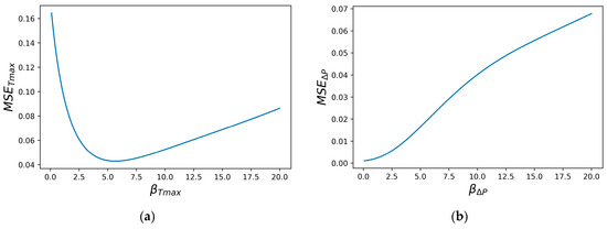
Figure 7.
The MSE tuning curves for the β hyper parameter: (a) ; (b) ∆P.
The maximum log likelihood strategy [74] is used to determine the hyperparameters of the GP models. These are presented in Table 8.
Table 8.
Configuration parameters for the GP ML approach.
Table 9 displays the MSE for each calibrated surrogate model. The GP model is best.
Table 9.
LOOCV MSE for each ML model.
5.2. Single-Objective Optimization
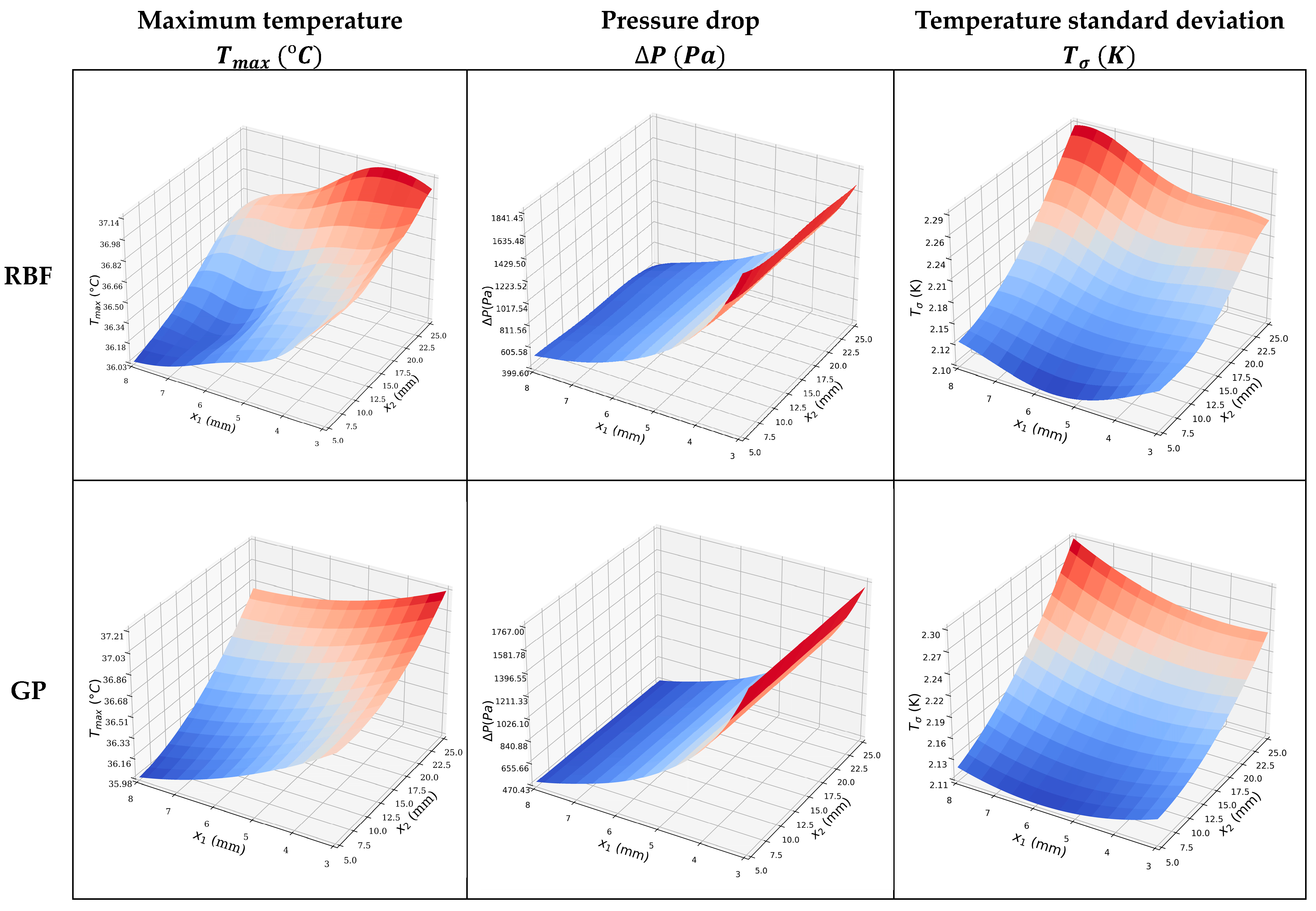
The surrogate models shown in Figure 8 are similar; however, the MSEs for the objective functions shown in Table 9 indicate that the GP model is more accurate. The single objective optimizations are straightforward, and the optima lie on the design space boundary. Those for the GP model are given in Table 10. Note that when is minimized, and are relatively large, indicating that it will be beneficial and interesting to perform multi-objective optimization.
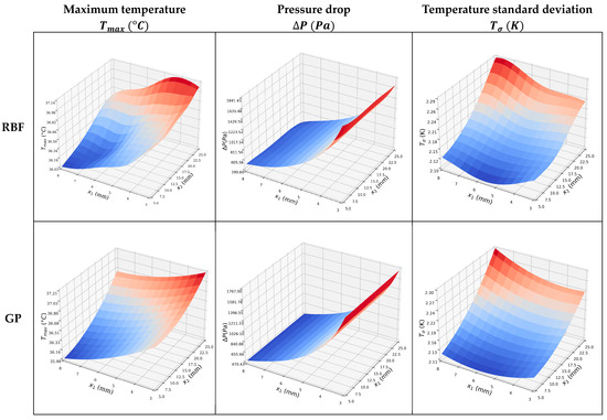
Figure 8.
Surrogate models of the , , and , using the two ML approaches.
Table 10.
Single objective optimization using the GP model.
5.3. Multi-Objective Optimization
Three two-dimensional Pareto fronts are constructed using the GP surrogate models within a generalized differential evolutionary algorithm (GDE3) [76] available in the pymoode Python package (v0.2.6). Li et al. [77] found that the GDE3 surpasses many different multi-objective optimization algorithms in terms of accuracy and chose it for their optimization study. The GDE3 algorithm setting parameters are listed in Table 11.
Table 11.
Basic GDE3 algorithm setting parameters.
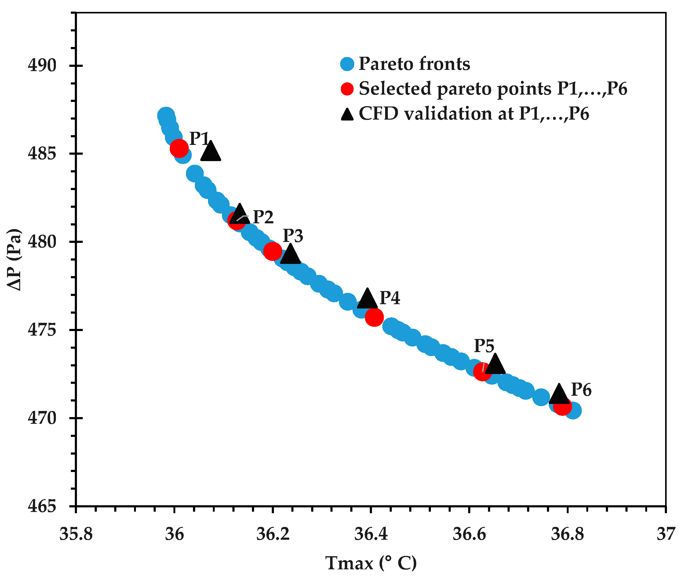
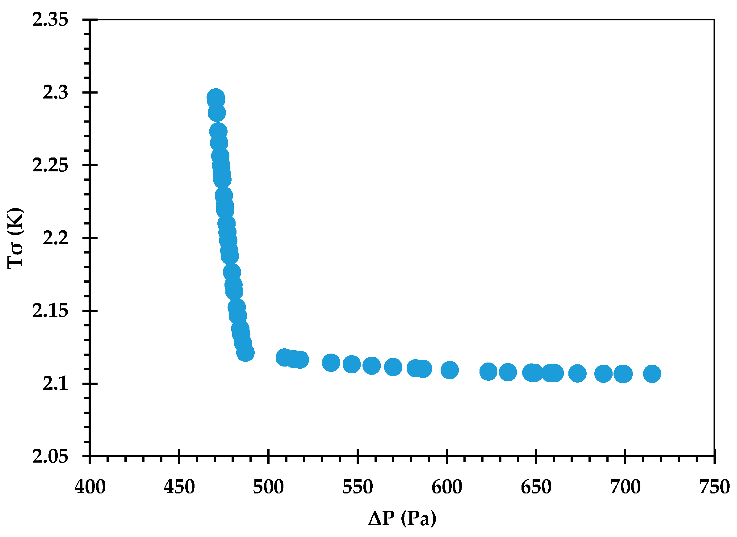
The Pareto front for against is shown in Figure 9, and its accuracy is verified by comparing some of the optimal points against corresponding CFD predictions in Table 12. An excellent agreement is observed, with the % error being <0.1 in all cases. Figure 10 provides the Pareto front for against . Figure 11 provides the Pareto front for against . These are useful for demonstrating the available compromises that designers can strike between the competing objectives. For instance, in Figure 9, decreasing from to would result in increasing from to . However, the increase in from around 36.0 to 36.2 in Figure 10 causes to drop from about 2.122 K to 2.107 K.
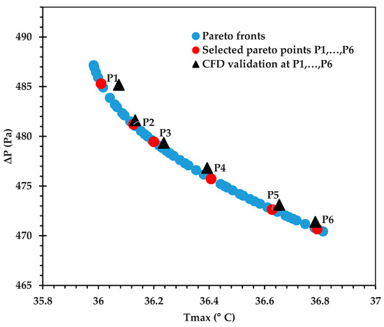
Figure 9.
Pareto curve of , obtained using the GP ML approach.
Table 12.
Validation of the objective functions at selected Pareto points with their corresponding CFD results, as seen in Figure 9.
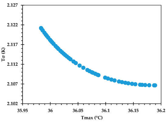
Figure 10.
Pareto curve of , obtained using the GP ML approach.
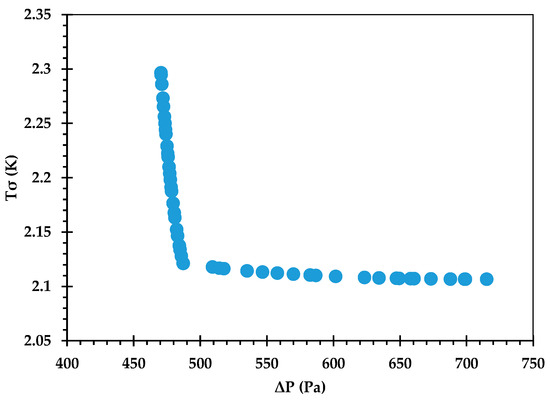
Figure 11.
Pareto curve of , obtained using the GP ML approach.
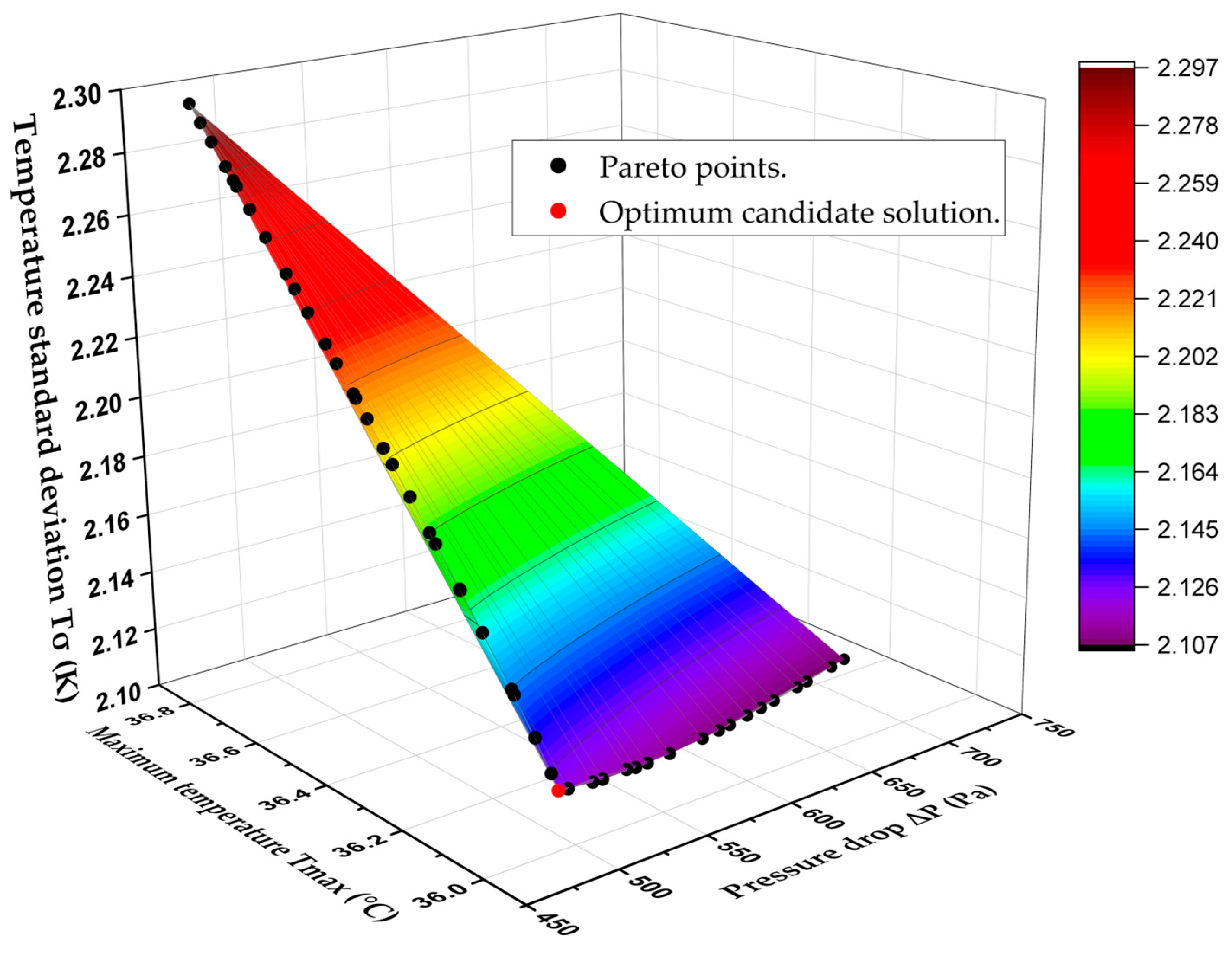
Finally, Figure 12 displays the 3D Pareto-optimal surface that is used to analyze trade-offs between the three competing objectives, , , and . The 3D Pareto-optimal surface’s accuracy is again verified by comparing a subset of the optimal points with corresponding CFD predictions, as shown in Table 13. The candidate point is chosen from among all non-dominated solutions and is located in the lower left corner of the pareto-optimal surface (See Figure 12). Table 14 shows a comparison between the optimum candidate design and the original (Benchmark) design of the BTMS. It also shows the performance enhancement, with the maximum temperature decreasing from 36.38 to 35.99 °C, the pressure drop dropping significantly from 782.82 to 494.41 Pa, and the temperature standard deviation reducing from 2.14 to 2.12 K.
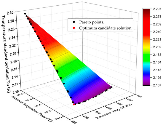
Figure 12.
3D Pareto-optimal surface to analyze trade-offs between , , and .
Table 13.
Validation of the objective functions for some Pareto surface points with their corresponding CFD results.
Table 14.
The final optimization results of the BTMS.
6. Conclusions
In this paper, a novel high-fidelity numerical simulation and MODO optimization methodology is developed and applied to the analysis and optimization of BTMS for Li-ion battery packs in electric vehicles for the first time. It is very important to simulate the complex, electro-chemical heat transfer mechanisms to provide accurate predictions of the time-dependent heat transfer generation and voltage profile in Li-ion battery packs. The present study has shown that this is very challenging due to the number of parameters, many of which are uncertain or missing in the literature, which need to be accounted for, and these simulations are computationally expensive, significantly increasing the time required for optimization studies. To aid future studies, the present study has provided a comprehensive and unambiguous list of the required modeling parameters.
Numerical simulation of the BTMS is carried out successfully using coupled P2D, 3D ECT, and conjugate heat transfer models that have been carefully validated against experimental and numerical data provided in references [28,49]. The coupled P2D-3D ECT modeling approach is used for the first time within a novel Gaussian process regression-enabled optimization methodology for Li-ion battery cooling using cold plates. The GP modeling is simple and effective to use and when combined with the GDE multi-objective algorithm allows the compromises, which can be achieved using cold plates, between the key objectives of battery maximum temperature (), temperature standard deviation (), and pressure drop () to be explored. The trade-offs between , , and are shown effectively using 2D Pareto fronts and a 3D Pareto-optimal surface. These multi-dimensional Pareto fronts can be used by designers to help them make more scientific decisions based on a careful analysis of the best options when dealing with conflicting objectives. For example, choosing design 2 over design 1 in Table 13 results in a temperature standard deviation that is lowered from 2.1212 to 2.1080 K, which is advantageous for a uniform temperature distribution. However, it significantly increases the pressure drop from 487.16 to 630.30 Pa and marginally boosts the battery’s maximum temperature from 35.983 to 36.113 °C. As a result, there are fewer concerns about battery safety, and more energy is required to pump the cooling water. The optimized BTMS provides better thermal efficiency and reduced pressure drop. The optimal candidate design provides the following improvements over the benchmark design: the battery’s maximum temperature drops from 36.38 to 35.98 °C, its standard temperature deviation decreases from 2.14 to 2.12 K, and the pressure drop dramatically decreases from 782.82 to 487.16 Pa. The corresponding optimum design parameters of the candidate point are the channel width of 8.00 mm and the horizontal spacing near the cold plate margin of 5.00 mm.
In future work, the modeling methodology developed here can be exploited in a range of different EV BTMSs based on liquid, boiling, and phase change materials. For example, continuing on from previous studies on heat sink cooling in electronics, there is a great scope of innovation in the design and optimization of minichannel designs within cold plates that could achieve substantial reductions in the magnitudes of the maximum temperature, temperature variations, and pressure drops with liquid-cooled cold plate-based BTMS. It would also be very interesting to combine the output of the research within a lifecycle assessment methodology where other key sustainability objectives, such as CO2 consumption, are optimized alongside the thermal and hydraulic objectives.
Author Contributions
Conceptualization, A.M. and H.T.; methodology, A.M.; software, A.M.; validation, A.M.; formal analysis, A.M.; investigation, A.M.; resources, A.M.; data curation, A.M.; writing—original draft preparation, A.M.; writing—review and editing, A.M., T.C., G.d.B., H.T. and J.V.; visualization, A.M.; supervision, T.C., G.d.B., H.T. and J.V.; project administration, T.C., G.d.B., H.T. and J.V.; funding acquisition, H.T. All authors have read and agreed to the published version of the manuscript.
Funding
This research was funded by the Higher Committee for Education Development in Iraq.
Data Availability Statement
The original contributions presented in the study are included in the article; further inquiries can be directed to the corresponding author.
Conflicts of Interest
The authors declare no conflicts of interest.
References
- Malima, G.C.; Moyo, F. Are electric vehicles economically viable in sub-Saharan Africa? The total cost of ownership of internal combustion engine and electric vehicles in Tanzania. Transp. Policy 2023, 141, 14–26. [Google Scholar] [CrossRef]
- Mehlig, D.; Staffell, I.; Stettler, M.; ApSimon, H. Accelerating electric vehicle uptake favours greenhouse gas over air pollutant emissions. Transp. Res. Part D Transp. Environ. 2023, 124, 103954. [Google Scholar] [CrossRef]
- Sopha, B.M.; Purnamasari, D.M.; Ma’mun, S. Barriers and Enablers of Circular Economy Implementation for Electric-Vehicle Batteries: From Systematic Literature Review to Conceptual Framework. Sustainability 2022, 14, 6359. [Google Scholar] [CrossRef]
- Ben Lazreg, M.; Baccouche, I.; Jemmali, S.; Manai, B.; Hamouda, M. State of Charge Estimation of Lithium-ion Battery in Electric Vehicles Using the Smooth Variable Structure Filter: Robustness Evaluation against Noise and Parameters Uncertainties. Electr. Power Compon. Syst. 2023, 51, 1630–1647. [Google Scholar] [CrossRef]
- Zhan, J.; Deng, Y.; Ren, J.; Gao, Y.; Liu, Y.; Rao, S.; Li, W.; Gao, Z. Cell Design for Improving Low-Temperature Performance of Lithium-Ion Batteries for Electric Vehicles. Batteries 2023, 9, 373. [Google Scholar] [CrossRef]
- Lu, L.; Han, X.; Li, J.; Hua, J.; Ouyang, M. A review on the key issues for lithium-ion battery management in electric vehicles. J. Power Sources 2013, 226, 272–288. [Google Scholar] [CrossRef]
- Hussain, A.; Tso, C.Y.; Chao, C.Y.H. Experimental investigation of a passive thermal management system for high-powered lithium ion batteries using nickel foam-paraffin composite. Energy 2016, 115, 209–218. [Google Scholar] [CrossRef]
- Panahi, M.; Heydari, H.R.; Karimi, G. Effects of micro heat pipe arrays on thermal management performance enhancement of cylindrical lithium-ion battery cells. Int. J. Energy Res. 2021, 45, 11245–11257. [Google Scholar] [CrossRef]
- Faraji, H.; Teggar, M.; Arshad, A.; Arıcı, M.; Mehdi Berra, E.; Choukairy, K. Lattice Boltzmann simulation of natural convection heat transfer phenomenon for thermal management of multiple electronic components. Therm. Sci. Eng. Prog. 2023, 45, 102126. [Google Scholar] [CrossRef]
- Babaharra, O.; Choukairy, K.; Faraji, H.; Hamdaoui, S. Improved heating floor thermal performance by adding PCM microcapsules enhanced by single and hybrid nanoparticles. Heat Transf. 2023, 52, 3817–3838. [Google Scholar] [CrossRef]
- Hwang, F.S.; Confrey, T.; Reidy, C.; Picovici, D.; Callaghan, D.; Culliton, D.; Nolan, C. Review of battery thermal management systems in electric vehicles. Renew. Sustain. Energy Rev. 2024, 192, 114171. [Google Scholar] [CrossRef]
- Amorim, G.S.; Belman-Flores, J.M.; de Paoli Mendes, R.; Sandoval, O.R.; Khosravi, A.; Garcia-Pabon, J.J. Recent advancements in thermal management technologies for cooling of data centers. J. Braz. Soc. Mech. Sci. Eng. 2024, 46, 472. [Google Scholar] [CrossRef]
- Nobrega, G.; Cardoso, B.; Souza, R.; Pereira, J.; Pontes, P.; Catarino, S.O.; Pinho, D.; Lima, R.; Moita, A. A Review of Novel Heat Transfer Materials and Fluids for Aerospace Applications. Aerospace 2024, 11, 275. [Google Scholar] [CrossRef]
- Do, N.B.D.; Imenes, K.; Aasmundtveit, K.E.; Nguyen, H.V.; Andreassen, E. Thermally Conductive Polymer Composites with Hexagonal Boron Nitride for Medical Device Thermal Management. In Proceedings of the 2023 24th European Microelectronics and Packaging Conference & Exhibition (EMPC), Hinxton, UK, 11–14 September 2023; pp. 1–8. [Google Scholar]
- Li, M.; Wang, J.; Chen, Z.; Qian, X.; Sun, C.; Gan, D.; Xiong, K.; Rao, M.; Chen, C.; Li, X. A Comprehensive Review of Thermal Management in Solid Oxide Fuel Cells: Focus on Burners, Heat Exchangers, and Strategies. Energies 2024, 17, 1005. [Google Scholar] [CrossRef]
- Akinlabi, A.A.H.; Solyali, D. Configuration, design, and optimization of air-cooled battery thermal management system for electric vehicles: A review. Renew. Sustain. Energy Rev. 2020, 125, 109815. [Google Scholar] [CrossRef]
- Luo, J.; Zou, D.; Wang, Y.; Wang, S.; Huang, L. Battery thermal management systems (BTMs) based on phase change material (PCM): A comprehensive review. Chem. Eng. J. 2022, 430, 132741. [Google Scholar] [CrossRef]
- Zhao, G.; Wang, X.; Negnevitsky, M.; Li, C. An up-to-date review on the design improvement and optimization of the liquid-cooling battery thermal management system for electric vehicles. Appl. Therm. Eng. 2023, 219, 119626. [Google Scholar] [CrossRef]
- An, Z.; Jia, L.; Li, X.; Ding, Y. Experimental investigation on lithium-ion battery thermal management based on flow boiling in mini-channel. Appl. Therm. Eng. 2017, 117, 534–543. [Google Scholar] [CrossRef]
- Zhao, C.; Zhang, B.; Zheng, Y.; Huang, S.; Yan, T.; Liu, X. Hybrid Battery Thermal Management System in Electrical Vehicles: A Review. Energies 2020, 13, 6257. [Google Scholar] [CrossRef]
- Tete, P.R.; Gupta, M.M.; Joshi, S.S. Developments in battery thermal management systems for electric vehicles: A technical review. J. Energy Storage 2021, 35, 102255. [Google Scholar] [CrossRef]
- Arora, S. Selection of thermal management system for modular battery packs of electric vehicles: A review of existing and emerging technologies. J. Power Sources 2018, 400, 621–640. [Google Scholar] [CrossRef]
- Katoch, S.S.; Eswaramoorthy, M. A Detailed Review on Electric Vehicles Battery Thermal Management System. IOP Conf. Ser. Mater. Sci. Eng. 2020, 912, 042005. [Google Scholar] [CrossRef]
- Tuckerman, D.B.; Pease, R.F.W. High-performance heat sinking for VLSI. IEEE Electron Device Lett. 1981, 2, 126–129. [Google Scholar] [CrossRef]
- Mitra, I.; Ghosh, I. Mini-channel heat sink parameter sensitivity based on precise heat flux re-distribution. Therm. Sci. Eng. Prog. 2020, 20, 100717. [Google Scholar] [CrossRef]
- Kewalramani, G.V.; Agrawal, A.; Saha, S.K. Modeling of microchannel heat sinks for electronic cooling applications using volume averaging approach. Int. J. Heat Mass Transf. 2017, 115, 395–409. [Google Scholar] [CrossRef]
- Li, W.; Peng, X.; Xiao, M.; Garg, A.; Gao, L. Multi-objective design optimization for mini-channel cooling battery thermal management system in an electric vehicle. Int. J. Energy Res. 2019, 43, 3668–3680. [Google Scholar] [CrossRef]
- Wang, N.; Li, C.; Li, W.; Chen, X.; Li, Y.; Qi, D. Heat dissipation optimization for a serpentine liquid cooling battery thermal management system: An application of surrogate assisted approach. J. Energy Storage 2021, 40, 102771. [Google Scholar] [CrossRef]
- Zhang, F.; He, Y.; Wang, C.; Liang, B.; Zhu, Y.; Gou, H.; Xiao, K.; Lu, F. A new type of liquid-cooled channel thermal characteristics analysis and optimization based on the optimal characteristics of 24 types of channels. Int. J. Heat Mass Transf. 2023, 202, 123734. [Google Scholar] [CrossRef]
- Li, W.; Wang, Y.; Yang, W.; Zhang, K. Design and optimization of an integrated liquid cooling thermal management system with a diamond-type channel. Therm. Sci. Eng. Prog. 2024, 47, 102325. [Google Scholar] [CrossRef]
- Dong, H.; Chen, X.; Yan, S.; Wang, D.; Han, J.; Guan, Z.; Cheng, Z.; Yin, Y.; Yang, S. Multi-Objective Optimization of the Thermal Management System for a Lithium-Ion Battery Pack with a Novel Bionic Lotus Leaf Channel is Performed Using Nsga-Ii and Rsm. SSRN 2023. Available online: https://ssrn.com/abstract=4621052 (accessed on 8 September 2024).
- Liu, F.; Chen, Y.; Qin, W.; Li, J. Optimal design of liquid cooling structure with bionic leaf vein branch channel for power battery. Appl. Therm. Eng. 2023, 218, 119283. [Google Scholar] [CrossRef]
- Wu, C.; Ni, J.; Shi, X.; Huang, R. A new design of cooling plate for liquid-cooled battery thermal management system with variable heat transfer path. Appl. Therm. Eng. 2024, 239, 122107. [Google Scholar] [CrossRef]
- Feng, S.; Shan, S.; Lai, C.; Chen, J.; Li, X.; Mori, S. Multi-objective optimization on thermal performance and energy efficiency for battery module using gradient distributed Tesla cold plate. Energy Convers. Manag. 2024, 308, 118383. [Google Scholar] [CrossRef]
- Sui, Z.; Lin, H.; Sun, Q.; Dong, K.; Wu, W. Multi-objective optimization of efficient liquid cooling-based battery thermal management system using hybrid manifold channels. Appl. Energy 2024, 371, 123766. [Google Scholar] [CrossRef]
- Ren, H.; Jia, L.; Dang, C.; Qi, Z. An electrochemical-thermal coupling model for heat generation analysis of prismatic lithium battery. J. Energy Storage 2022, 50, 104277. [Google Scholar] [CrossRef]
- Kim, U.S.; Yi, J.; Shin, C.B.; Han, T.; Park, S. Modelling the thermal behaviour of a lithium-ion battery during charge. J. Power Sources 2011, 196, 5115–5121. [Google Scholar] [CrossRef]
- Gan, Y.; Wang, J.; Liang, J.; Huang, Z.; Hu, M. Development of thermal equivalent circuit model of heat pipe-based thermal management system for a battery module with cylindrical cells. Appl. Therm. Eng. 2020, 164, 114523. [Google Scholar] [CrossRef]
- Hou, G.; Liu, X.; He, W.; Wang, C.; Zhang, J.; Zeng, X.; Li, Z.; Shao, D. An equivalent circuit model for battery thermal management system using phase change material and liquid cooling coupling. J. Energy Storage 2022, 55, 105834. [Google Scholar] [CrossRef]
- Gao, Z.; Chin, C.S.; Woo, W.L.; Jia, J. Integrated Equivalent Circuit and Thermal Model for Simulation of Temperature-Dependent LiFePO4 Battery in Actual Embedded Application. Energies 2017, 10, 85. [Google Scholar] [CrossRef]
- Doyle, M.; Fuller, T.F.; Newman, J. Modeling of Galvanostatic Charge and Discharge of the Lithium/Polymer/Insertion Cell. J. Electrochem. Soc. 1993, 140, 1526. [Google Scholar] [CrossRef]
- Liu, J.; Yadav, S.; Salman, M.; Chavan, S.; Kim, S.C. Review of thermal coupled battery models and parameter identification for lithium-ion battery heat generation in EV battery thermal management system. Int. J. Heat Mass Transf. 2024, 218, 124748. [Google Scholar] [CrossRef]
- Mevawalla, A.; Panchal, S.; Tran, M.-K.; Fowler, M.; Fraser, R. Mathematical Heat Transfer Modeling and Experimental Validation of Lithium-Ion Battery Considering: Tab and Surface Temperature, Separator, Electrolyte Resistance, Anode-Cathode Irreversible and Reversible Heat. Batteries 2020, 6, 61. [Google Scholar] [CrossRef]
- Guo, S.; Li, J.; Wang, Y.; Wang, Z. Electrochemical-thermal coupling model of lithium-ion battery at ultra-low temperatures. Appl. Therm. Eng. 2024, 240, 122205. [Google Scholar] [CrossRef]
- An, F.; Zhou, W.; Li, P. A comparison of model prediction from P2D and particle packing with experiment. Electrochim. Acta 2021, 370, 137775. [Google Scholar] [CrossRef]
- Hariharan, K.S.; Tagade, P.; Ramachandran, S. Mathematical Modeling of Lithium Batteries from Electrochemical Models to State Estimator Algorithms, 1st ed.; Springer: Cham, Switzerland, 2018. [Google Scholar]
- Newman, J.; Tiedemann, W. Porous-electrode theory with battery applications. AIChE J. 1975, 21, 25–41. [Google Scholar] [CrossRef]
- Newman, J.; Thomas-Alyea, K.E. Electrochemical Systems, 3rd ed.; Wiley: Hoboken, NJ, USA, 2004. [Google Scholar]
- Ning, G.; Popov, B.N. Cycle Life Modeling of Lithium-Ion Batteries. J. Electrochem. Soc. 2004, 151, A1584. [Google Scholar] [CrossRef]
- Guo, M.; Sikha, G.; White, R.E. Single-Particle Model for a Lithium-Ion Cell: Thermal Behavior. J. Electrochem. Soc. 2011, 158, A122. [Google Scholar] [CrossRef]
- Jin, N.; Danilov, D.L.; Van den Hof, P.M.J.; Donkers, M.C.F. Parameter estimation of an electrochemistry-based lithium-ion battery model using a two-step procedure and a parameter sensitivity analysis. Int. J. Energy Res. 2018, 42, 2417–2430. [Google Scholar] [CrossRef]
- Panchal, S.; Dincer, I.; Agelin-Chaab, M.; Fraser, R.; Fowler, M. Transient electrochemical heat transfer modeling and experimental validation of a large sized LiFePO4/graphite battery. Int. J. Heat Mass Transf. 2017, 109, 1239–1251. [Google Scholar] [CrossRef]
- Wang, M.; Li, J.; He, X.; Wu, H.; Wan, C. The effect of local current density on electrode design for lithium-ion batteries. J. Power Sources 2012, 207, 127–133. [Google Scholar] [CrossRef]
- Xu, M.; Zhang, Z.; Wang, X.; Jia, L.; Yang, L. A pseudo three-dimensional electrochemical–thermal model of a prismatic LiFePO4 battery during discharge process. Energy 2015, 80, 303–317. [Google Scholar] [CrossRef]
- Di Domenico, D.; Stefanopoulou, A.; Fiengo, G. Lithium-Ion Battery State of Charge and Critical Surface Charge Estimation Using an Electrochemical Model-Based Extended Kalman Filter. J. Dyn. Syst. Meas. Control. 2010, 132, 061302. [Google Scholar] [CrossRef]
- Arora, P.; Doyle, M.; White, R.E. Mathematical Modeling of the Lithium Deposition Overcharge Reaction in Lithium-Ion Batteries Using Carbon-Based Negative Electrodes. J. Electrochem. Soc. 1999, 146, 3543. [Google Scholar] [CrossRef]
- Nazari, A.; Farhad, S. Heat generation in lithium-ion batteries with different nominal capacities and chemistries. Appl. Therm. Eng. 2017, 125, 1501–1517. [Google Scholar] [CrossRef]
- Cai, L.; White, R.E. Mathematical modeling of a lithium ion battery with thermal effects in COMSOL Inc. Multiphysics (MP) software. J. Power Sources 2011, 196, 5985–5989. [Google Scholar] [CrossRef]
- Chen, C.-H.; Brosa Planella, F.; O’Regan, K.; Gastol, D.; Widanage, W.D.; Kendrick, E. Development of Experimental Techniques for Parameterization of Multi-scale Lithium-ion Battery Models. J. Electrochem. Soc. 2020, 167, 080534. [Google Scholar] [CrossRef]
- Xu, M.; Wang, R.; Reichman, B.; Wang, X. Modeling the effect of two-stage fast charging protocol on thermal behavior and charging energy efficiency of lithium-ion batteries. J. Energy Storage 2018, 20, 298–309. [Google Scholar] [CrossRef]
- Bizeray, A. State and Parameter Estimation of Physics-Based Lithium-Ion Battery Models; University of Oxford: Oxford, UK, 2016. [Google Scholar]
- Comsol Multiphysics v.6.0, Heat Transfer Module User’s Guide; COMSOL AB: Stockholm, Sweden, 2023; Available online: https://www.comsol.com (accessed on 8 September 2024).
- Fan, Y.; Wang, Z.; Xiong, X.; Panchal, S.; Fraser, R.; Fowler, M. Multi-Objective Optimization Design and Experimental Investigation for a Prismatic Lithium-Ion Battery Integrated with a Multi-Stage Tesla Valve-Based Cold Plate. Processes 2023, 11, 1618. [Google Scholar] [CrossRef]
- Liu, H.; Gao, X.; Niu, D.; Yu, M.; Ji, Y. Thermal-Hydraulic Characteristics of the Liquid-Based Battery Thermal Management System with Intersected Serpentine Channels. Water 2022, 14, 3148. [Google Scholar] [CrossRef]
- Sheng, L.; Su, L.; Zhang, H.; Li, K.; Fang, Y.; Ye, W.; Fang, Y. Numerical investigation on a lithium ion battery thermal management utilizing a serpentine-channel liquid cooling plate exchanger. Int. J. Heat Mass Transf. 2019, 141, 658–668. [Google Scholar] [CrossRef]
- Wang, Q.-K.; Shen, J.-N.; Ma, Z.-F.; He, Y.-J. Decoupling parameter estimation strategy based electrochemical-thermal coupled modeling method for large format lithium-ion batteries with internal temperature experimental validation. Chem. Eng. J. 2021, 424, 130308. [Google Scholar] [CrossRef]
- Liu, Y.; Wang, X.; Wang, L. Interval uncertainty analysis for static response of structures using radial basis functions. Appl. Math. Model. 2019, 69, 425–440. [Google Scholar] [CrossRef]
- Nie, Y.; Du, Y.; Xu, Z.; Zhang, Z.; Qi, Y. RBF Interpolation Algorithm for FTS Tool Path Generation. Math. Probl. Eng. 2021, 2021, 6689200. [Google Scholar] [CrossRef]
- Hamad, H.S.; Kapur, N.; Khatir, Z.; Querin, O.M.; Thompson, H.M.; Wang, Y.; Wilson, M.C.T. Computational fluid dynamics analysis and optimisation of polymerase chain reaction thermal flow systems. Appl. Therm. Eng. 2021, 183, 116122. [Google Scholar] [CrossRef]
- Wang, J. An Intuitive Tutorial to Gaussian Processes Regression. Comput. Sci. Eng. 2023, 25, 4–11. [Google Scholar] [CrossRef]
- Xu, P.; Ji, X.; Li, M.; Lu, W. Small data machine learning in materials science. NPJ Comput. Mater. 2023, 9, 42. [Google Scholar] [CrossRef]
- Dhamodharavadhani, S.; Rathipriya, R. Novel COVID-19 Mortality Rate Prediction (MRP) Model for India Using Regression Model With Optimized Hyperparameter. J. Cases Inf. Technol. (JCIT) 2021, 23, 1–12. [Google Scholar] [CrossRef]
- Yan, X.; Liu, D.; Xu, W.; He, D.; Hao, H. Hydraulic fracturing performance analysis by the mutual information and Gaussian process regression methods. Eng. Fract. Mech. 2023, 286, 109285. [Google Scholar] [CrossRef]
- Martins, J.R.R.A.; Ning, A. Engineering Design Optimization; Cambridge University Press: Cambridge, UK, 2021. [Google Scholar]
- Duvenaud, D. Automatic Model Construction with Gaussian Processes. Ph.D. Thesis, University of Cambridge, Cambridge, UK, 2014. [Google Scholar]
- Leite, B.; Costa, A.O.S.d.; Costa Junior, E.F.d. Multi-objective optimization of adiabatic styrene reactors using Generalized Differential Evolution 3 (GDE3). Chem. Eng. Sci. 2023, 265, 118196. [Google Scholar] [CrossRef]
- Li, Y.; Li, C.; Garg, A.; Gao, L.; Li, W. Heat dissipation analysis and multi-objective optimization of a permanent magnet synchronous motor using surrogate assisted method. Case Stud. Therm. Eng. 2021, 27, 101203. [Google Scholar] [CrossRef]


Disclaimer/Publisher’s Note: The statements, opinions and data contained in all publications are solely those of the individual author(s) and contributor(s) and not of MDPI and/or the editor(s). MDPI and/or the editor(s) disclaim responsibility for any injury to people or property resulting from any ideas, methods, instructions or products referred to in the content. |
© 2024 by the authors. Licensee MDPI, Basel, Switzerland. This article is an open access article distributed under the terms and conditions of the Creative Commons Attribution (CC BY) license (https://creativecommons.org/licenses/by/4.0/).