Abstract
Discrepancies between laboratory vehicle performance and real-world traffic conditions have been reported in numerous studies. In response, emission and fuel regulatory frameworks started incorporating real-world traffic evaluations and vehicle monitoring using portable emissions measurement systems (PEMS) and on-board diagnostic (OBD) data. However, in regions with technical and economic constraints, such as Latin America, the use of PEMS is often limited, highlighting the need for low-cost methodologies to assess vehicle performance. OBD interfaces provide extensive vehicle and engine operational data in this context, offering a valuable alternative for analyzing vehicle performance in real-world conditions. This study proposes a straightforward methodology for assessing vehicle fuel efficiency and carbon dioxide (CO2) emissions under real-world traffic conditions using OBD data. An experimental campaign was conducted with three gasoline-powered passenger vehicles representative of the Ecuadorian fleet, operating as urban taxis in Ibarra, Ecuador. This methodology employs an OBD interface paired with a mobile phone data logging application to capture vehicle kinematics, engine parameters, and fuel consumption. These data were used to develop engine maps and assess vehicle performance using the vehicle-specific power (VSP) approach based on the energy required for vehicle propulsion. Additionally, VSP analysis combined with OBD data facilitated the development of an energy-emission model to characterize fuel consumption and CO2 emissions for the tested vehicles. The results demonstrate that OBD systems effectively monitor vehicle performance in real-world conditions, offering crucial insights for improving urban transportation sustainability. Consequently, OBD data serve as a critical resource for research supporting decarbonization efforts in Latin America.
1. Introduction
Urban transportation significantly contributes to greenhouse gas (GHG) emissions and air pollution in cities worldwide, presenting critical environmental and public health challenges. Global energy consumption for road transport is expected to rise by 28% between 2022 and 2050, signaling a worsening scenario in pollution [1]. In Latin America, the energy–mix is predominantly fossil fuel-based, accounting for approximately 65% of the region’s total energy matrix. Road transport is the primary GHG emitter in the region, consuming nearly 37% of the total energy supply [2]. Addressing emissions from road transport is thus an urgent task that requires considering each region’s unique political, social, technical, and economic context.
In each region, vehicle performance and engine efficiency are influenced by various factors, which can be categorized into four main groups: (i) vehicle characteristics (exogenous factors like fuel type, engine condition, and engine load level; and endogenous factors like engine speed, powertrain configuration, and air/fuel mixture) [3], (ii) driver behavior (e.g., driving style, gear-shifting pattern) [4], (iii) traffic conditions (e.g., average speed, number of stops) [5], and (iv) road conditions (endogenous factors like road type, road grade, intersection signal configuration; and exogenous factors like altitude, ambient temperature, humidity) [6,7]. In Latin America, unique regional factors also play a significant role. For instance, cities in Andean countries such as Ecuador, Colombia, and Peru are often situated in mountainous regions at altitudes exceeding 2000 m above sea level. Additionally, the vehicle technology in these markets tends to be less advanced than in Europe or the United States. These regional differences significantly impact vehicle emissions and fuel efficiency, highlighting the need for tailored solutions.
Implementing emission standards and fuel regulations has driven advancements in testing procedures and equipment over recent decades. Initially, vehicles were tested under controlled laboratory conditions using chassis dynamometers and constant volume sampler (CVS) gas analyzers to measure diluted emissions, especially for light-duty vehicles (LDVs). For heavy-duty vehicles (HDVs), engine testing was conducted on engine benches with CVS analyzers [8]. However, discrepancies between laboratory vehicle performances and real-world traffic conditions were reported in several studies. As a result, starting in 2015, regulatory frameworks began including real-world traffic evaluations and monitoring using portable emissions measurement systems (PEMS) and on-board diagnostic (OBD) data [9,10]. Laboratory testing also evolved to incorporate more demanding driving cycles, such as the Worldwide Harmonized Light Vehicles Test Cycle (WLTC) [11,12]. Additionally, regulatory authorities now propose vehicle assessments before and after commercialization, including “In-Service Conformity” (ISC) tests [13]. Despite these advances, regulatory changes are not progressing simultaneously across all regions. Only countries like Chile and Brazil have a clear roadmap for adopting Euro IV-equivalent regulations in Latin America. In contrast, countries like Ecuador and Costa Rica still rely on Euro II and III standards [14]. Given the limited access to PEMS equipment, OBD data provide a valuable alternative for analyzing vehicle performance under real-world conditions in the region.
Researchers utilize various methodologies to monitor and assess vehicle emissions, including emission modeling, vehicle simulators, the vehicle-specific power (VSP) approach—which accounts for the vehicle’s tractive energy—engine map development, and real-world testing using PEMS [15]. Each method has unique advantages and applications. For example, advanced mathematical models were developed to estimate fuel consumption in flexible fuel vehicle engines by considering fundamental fuel properties [16]. The VSP approach was used to assess heavy vehicles’ driving cycle distributions and emissions, offering insights into their environmental impact [17]. The PEMS-based experimental data were utilized to analyze real-world traffic emissions for taxis powered by gasoline and biofuel in various Chinese cities, highlighting the variability in urban driving conditions [18]. Machine learning techniques, such as Artificial Neural Networks (ANN), were also employed to model a six-cylinder marine diesel engine by mapping its thermal performance characteristics [19]. Furthermore, comprehensive procedures for creating engine maps using dynamometer test data were established, allowing a detailed vehicle performance simulation [20].
In Latin America, evaluating vehicle performance under real-world traffic conditions is often limited by technical and economic constraints [21]. In countries like Ecuador, vehicle homologation processes, where state agencies must verify a vehicle’s performance before commercialization, are often conducted solely through documentation, bypassing actual laboratory or road tests. Moreover, many countries in the region have yet to establish emission factors in terms of mass (g/km), and outdated legislation continues to assess vehicle performance based on emission concentrations (ppm, %V). The poor fuel quality further hinders governments from implementing stricter emission standards [22]. Monitoring and controlling in-use vehicles through ISC tests are also largely absent. Given these challenges, low-cost methodologies for evaluating vehicle performance are highly recommended for Latin America. Using cost-effective OBD interfaces, which provide access to extensive vehicle information like engine performance data, exhaustive after-treatment system status, and various operational parameters, are valuable tools for researchers and policymakers in the region. OBD systems, already regulated in regions like Europe and the United States [12,23], are reliable for assessing and monitoring vehicles operating under real-world traffic conditions. Therefore, OBD data serve as a crucial resource for studies supporting the decarbonization efforts in Latin America.
This research makes a significant contribution by addressing the gaps in the current literature by developing a straightforward and low-cost methodology for assessing vehicle fuel efficiency and carbon dioxide (CO2) emissions under real-world traffic conditions using OBD data. It provides practical insights to improve the sustainability of urban transport, especially in regions with technical and economic limitations like Latin America. The methodology encompasses three key aspects: (i) generating engine maps using OBD data collected during real-world driving; (ii) comparing vehicle performance through engine operation patterns and the VSP approach; (iii) and developing and evaluating a VSP-based emissions model for characterizing fuel consumption and CO2 emissions in Latin American traffic. An experimental campaign involved three gasoline passenger vehicles representative of the Ecuadorian fleet, tested during urban taxi operations in Ibarra, Ecuador. The data on vehicle kinematics, engine parameters, and fuel consumption were collected using an OBD-II interface connected to a mobile phone application, with navigation data referenced via a global positioning system (GPS) logger.
The remainder of this paper is organized as follows. Section 2 discusses the roles and functions of PEMS and OBDs in emission monitoring. Section 3 details the proposed methodology, including the experimental setup and procedures. Section 4 discusses the results and their implications. Finally, Section 5 concludes the paper and suggests avenues for future research.
2. PEMS and OBD
PEMS and OBD systems are two crucial vehicle emission monitoring and control technologies. These systems provide essential data that enhance the understanding of vehicle performance under real-world conditions, facilitating more effective regulatory compliance and emission reduction strategies.
PEMS are advanced devices designed to measure and record on-board vehicle emissions on a second-by-second basis in real time under real-world operating conditions [24]. As detailed in Table 1, PEMS consist of several key components, including emission sensors, a data acquisition system, a GPS, an on-board computer, and a power supply. The emission sensors detect and measure the concentrations of gaseous pollutants such as CO2, nitrous oxides (NOx), carbon monoxide (CO), and total hydrocarbon (THC). The data acquisition system collects and stores this information for subsequent analysis. The GPS unit records the vehicle’s location, allowing for a contextual emission data analysis. The on-board computer integrates and processes the collected data, generating comprehensive reports on vehicle emission performance. The power supply ensures the continuous operation of the PEMS components.

Table 1.
Operation of PEMS.
Conversely, OBD systems are crucial for diagnosing and monitoring vehicle performance and emission control systems [25]. Table 2 summarizes the key components and functions of OBD systems. The core of the OBD system is the engine control module (ECM), which monitors engine performance and exhaust gas treatment processes. A network of sensors throughout the vehicle collects engine and exhaust condition data, which the ECM uses to monitor and regulate these systems. The diagnostic interface allows the connection of external diagnostic tools, enabling the retrieval and analysis of stored performance data and fault data from the ECM. Additionally, the malfunction indicator light (MIL) alerts drivers to detected faults, while the fault code log stores specific diagnostic codes for identified problems, enabling the accurate identification and resolution of technical issues.
Table 2.
Operation of OBD systems.
Overall, PEMS and OBD systems offer comprehensive tools for monitoring and controlling vehicle emissions. These systems are designed to address all aspects of emissions and control, providing an all-encompassing solution. PEMS are particularly effective for capturing emission data during real-world driving conditions, while OBD systems deliver detailed diagnostics and continuous performance monitoring. Integrating these technologies is essential for ensuring that vehicles meet emission standards and developing strategies to reduce overall vehicle emissions. However, in Latin America, where access to PEMS equipment is limited, using OBD systems is a viable and cost-effective alternative for assessing fuel efficiency and CO2 emissions under real-world operating conditions.
3. Proposed Methodology
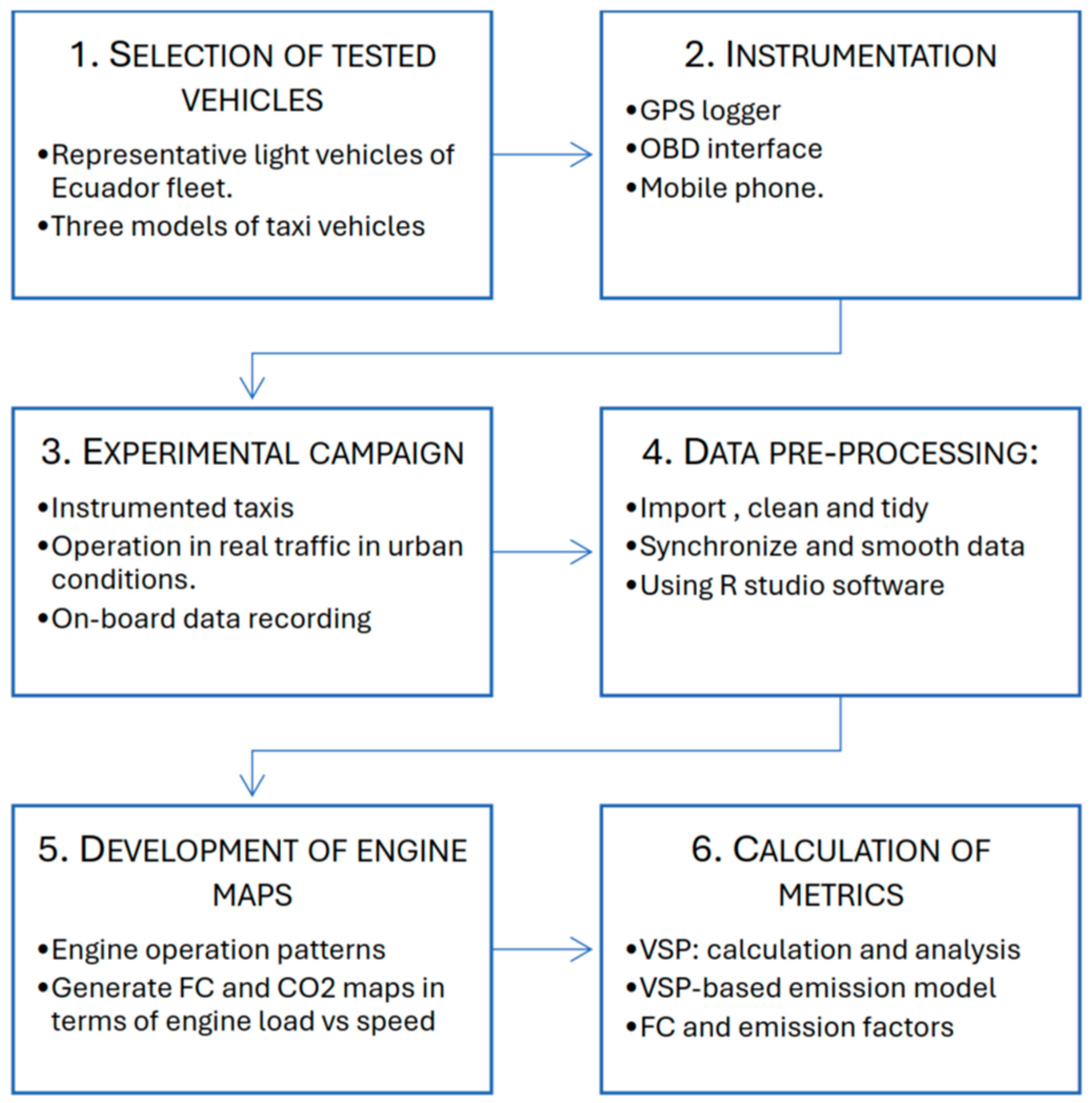
The proposed methodology, shown in Figure 1, encompasses several crucial stages for assessing vehicle fuel efficiency and CO2 emissions under real-world traffic conditions. This methodology is tested through an experiment that follows these outlined steps:
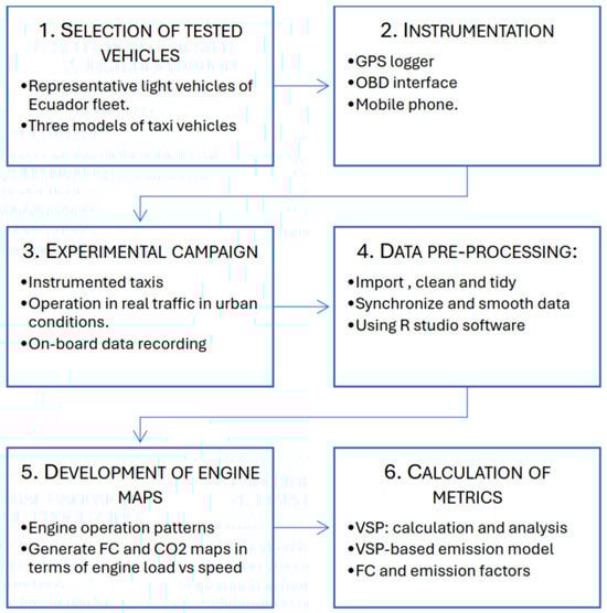
Figure 1.
The methodology proposed in this study for the vehicle emissions analysis process.
- Vehicles representative of the local fleet are chosen for analysis. The vehicles’ real-world traffic operation is recorded while they function as urban transportation (city taxi service) rather than being tested on a specific route.
- A GPS logger and an OBD interface connected to a mobile phone application are installed to collect real-time data on vehicle and engine operating parameters, enabling the recording of critical data required to analyze fuel consumption and CO2 emissions.
- The instrumented vehicles are driven on various routes based on demand from taxi users, primarily in urban areas, to collect data representative of real-world driving scenarios.
- The collected data from the GPS logger and OBD interface undergo synchronization and smoothing processes to ensure the accuracy and reliability for subsequent analysis.
- Engine maps are generated to visualize the relationship between engine load, speed, and performance parameters (e.g., fuel consumption and CO2 rates). This involves creating grid maps for engine load and speed ranges and plotting two-dimensional contour maps based on the collected data.
- Metrics such as the relative frequency of engine speed and load, VSP values, fuel efficiency, and CO2 emission factors are calculated using the collected data and developed engine maps.
Although this study did not directly validate OBD-derived fuel consumption estimates against actual vehicle fuel consumption using PEMS or flow meters, previous research demonstrated the reliability of OBD data. Studies showed that errors associated with OBD fuel consumption estimates for spark ignition and diesel vehicles typically remain below 4% [25,26]. Moreover, the use of OBD data has been widely regulated by international legislation [12,23], reinforcing its credibility as a tool for vehicle performance assessment. Despite the absence of direct validation in this study, the methodology remains a cost-effective and scientifically robust approach, especially valuable for regions with limited access to more advanced technologies like PEMS. This makes the OBD-based approach particularly applicable for real-world emissions analysis in resource-constrained areas, such as Latin America, where cost-effective yet accurate methodologies are essential.
3.1. Selection of Tested Vehicles
Three gasoline-powered passenger vehicles—Chevrolet Aveo Activo, Chevrolet Sail, and Hyundai Accent—were selected to serve as taxis representing the Ecuadorian fleet. These vehicles were chosen for their suitability for fuel consumption analysis through the OBD II system and because they align with the typical passenger capacity, weight, engine torque, power, and gearbox configurations standard in Ecuador’s automotive segment. In Ecuador, the transport sector consumes 49% of the total energy, primarily from diesel and gasoline, and grows annually by up to 25% [27]. This sector was responsible for approximately 50% of the country’s GHG emissions in 2021. The taxi drivers participate voluntarily, providing a reliable basis for analysis. Detailed specifications of the tested vehicles are presented in Table 3.
Table 3.
Technical specifications of the tested vehicles.
3.2. Instrumentation
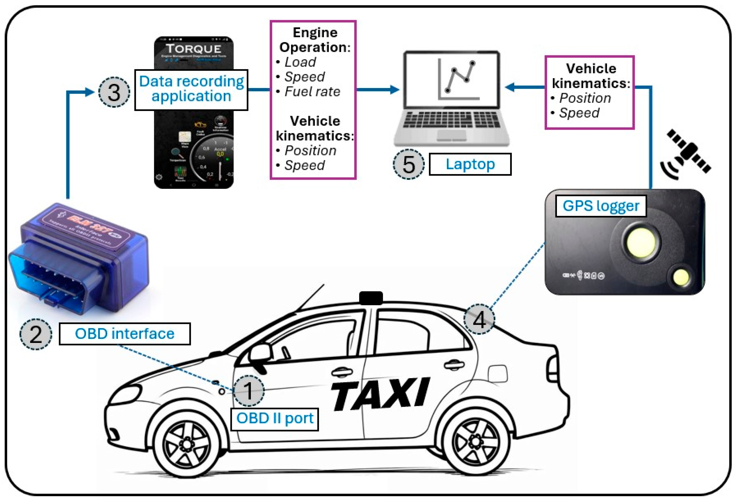
Instruments are required to measure three types of information: vehicle kinematics (e.g., position and speed), vehicle and engine operating parameters (e.g., engine load and speed values), and instantaneous fuel consumption rate data. A GPS logger device, the GL-770, was installed in the test vehicles to record latitude, longitude, altitude, and time at 1 Hz. This device was non-intrusive, allowing the collection of vehicle kinematic information without altering the ordinary course of operation of tested vehicles. Additionally, an OBD interface device, the ELM Electronics 327, was connected to a mobile phone application named Torque Pro to record vehicle fuel consumption data and engine operating parameters. Overall, the ELM 327 connects to the vehicle’s ECU via the OBD2 diagnostic port, reading its operating parameters in real time and sending them via Bluetooth to the Torque Pro application.
The ELM Electronics 327 interface is a diagnostic tool designed for vehicles equipped with OBD II and CAN systems, commonly found in vehicles manufactured after 1996 in the United States, Europe, and Asia, with a 16-pin diagnostic connector. This interface can read diagnostic trouble codes (DTCs), clear them, and retrieve real-time sensor data from the engine through the vehicle’s ECM [28]. Additionally, the ELM 327 could turn off the check engine light by clearing DTCs and providing information on the sensors installed in the vehicle. It offers a real-time display of sensor data such as intake manifold pressure, engine speed, vehicle speed, fuel system status, air flow rate, oxygen sensors, and the fuel consumption rate. This interface is compatible with many OBD II-compliant vehicles [25,26]. This device typically uses wireless communication methods like Bluetooth or Wi-Fi, making it highly versatile for monitoring vehicle performance under real-world driving conditions.
The mobile application Torque Pro is a versatile diagnostic tool for real-time vehicle performance monitoring through an OBD-II interface, such as ELM327. It enables users to access and log data such as engine speed, fuel consumption, and kinematic vehicle parameters. Additionally, Torque Pro allows users to read and interpret DTCs generated by a vehicle’s systems when issues arise. With access to detailed sensor data and parameter identification codes (PIDs), the mobile application offers advanced diagnostic and monitoring capabilities, making it ideal for assessing vehicle performance under real-world operating conditions.
Figure 2 illustrates the schematic of the instrument installation used to evaluate the performance of the taxis. The installation of the ELM 327 interface with the Torque Pro application was completed through the following seven steps: (i) the ELM 327 interface was connected to the OBDII port of the tested vehicle to extract the data from the ECM; (ii) the Torque Pro application was installed on a mobile device, which served as the primary data recording platform; (iii) a Bluetooth pairing was established between the ELM 327 interface and the mobile device to enable data transmission; (iv) Torque Pro was launched, and the OBDII adapter connection type was configured to Bluetooth, ensuring seamless communication with the interface; (v) the connection was verified to ensure the successful data reception from the vehicle; (vi) specific PIDs were selected within Torque Pro for recording, focusing on critical variables such as vehicle kinematics (e.g., longitude, latitude, altitude, distance, GPS speed, and wheel speed sensor) and engine operation parameters (e.g., engine load, engine speed, throttle position, intake manifold pressure, intake air temperature, and engine coolant temperature); and (vii) Torque Pro was configured to record data at a frequency of 1 Hz. After completing these configurations, the OBD interface and mobile application were available to start data recording for the experimental campaign. Notably, the GPS logger GL-770 operated independently, capturing positional data separately from the OBD system, enabling a comprehensive data collection to assess vehicle emissions and fuel efficiency under real-world driving conditions.
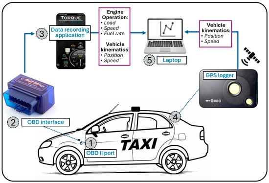
Figure 2.
Schematic of the instrumentation.
3.3. Experimental Campaign
The experimental campaign was conducted in Ibarra, Ecuador, a city in the Imbabura province with approximately 200,000 residents. Due to a significant annual growth rate of around 8%, the city faces challenges with traffic management and mobility, which includes approximately 90% of urban conditions (0–60 km/h). The remaining 10% includes suburban areas (60–90 km/h) and highways (>90 km/h). This approach was designed to collect data representative of real-world driving situations.
The campaign began with the meticulous installation and assembly of monitoring equipment, following in-depth discussions with members of a taxi company who voluntarily participated in the project. The data collection process was carefully planned, with two weeks allocated for this purpose. The data was collected in February, covering peak and off-peak hours, using three taxi models running on commercially available gasoline. Before each session, the taxis were warmed up for at least 30 min to ensure optimal operating conditions. A single driver operated each taxi throughout this study to minimize variability due to driving style. Consistent weather conditions during the tests helped mitigate the influence of environmental factors. Additionally, the taxis’ air conditioning systems were activated during all tests. Table 4. provides an overview of the operating conditions for the tested vehicles during the experimental campaign.
Table 4.
Overview of the operating conditions for tested vehicles in the experimental campaign.
3.4. Data Pre-Processing
Data pre-processing used R Studio software version 2023.12.1 to address the differences in initial recording times between the GPS and OBD devices used in the experimental campaign. The pre-processing involved synchronizing the signals from these devices based on vehicle speed, which was recorded second-by-second. The speed profiles were then smoothed using a moving window filter, ensuring the accuracy and reliability of the results presented in this study.
3.5. Development of Engine Maps
Developing an engine map requires three key variables. Commonly, torque and engine speed serve as the axes for the engine maps. At the same time, a third variable (e.g., brake thermal efficiency (BTE), fuel consumption, and emission rates) defines the map’s specific focus. The methodology for engine map development involved two primary stages: (i) creating grid engine maps based on ranges of engine load and speed with averaged data values and (ii) generating two-dimensional contour maps from the grid data. These processes were carried out using R Studio.
The construction of grid engine maps was based on the methodology outlined in [29]. First, grids were established according to predefined engine load and speed intervals, after which the remaining operational data (the third variable) were assigned to their respective grids. The data within each grid were then averaged to produce a single representative value for each speed–load combination. Outliers were identified and removed by analyzing each data group’s relative frequency and standard deviation. Once filtered, the averaged data were discretized for color visualization on the engine maps. Then, to create the contour engine maps, R Studio with the ggplot2 R package was used [30,31]. The data from the grid maps served as the input for generating these contours. The third variable’s intervals were clearly defined to improve visualization, and a divergent color scheme was employed. This approach resulted in detailed contour maps for various engine parameters, including BTE, brake-specific fuel consumption (BSFC), brake-specific CO2 emissions, fuel consumption, and CO2 emission rates.
3.6. Calculation of Metrics
3.6.1. Estimation of CO2 Emission Rates
The CO2 emission rate for each tested vehicle was calculated by
which is derived from the stoichiometric combustion of gasoline (C8H18). Given that the fuel used is gasoline, the assumed values were 18 for hydrogen (H) and 8 for carbon (C). The instantaneous fuel consumption rate was expressed in (g/s), serving as the basis for determining the CO2 emission rate.
3.6.2. Fuel Consumption and Emission Factors
To estimate the performance of the tested vehicles, their distance-specific fuel consumption and CO2 emissions factors were calculated by
where is the estimated distance-specific FC for each tested vehicle ; is the distance travelled; and is the total time of travel. In Equation (3), is the estimated distance-specific CO2 emission factor by vehicle , while is the instantaneous CO2 emission rate expressed in (g/s).
3.6.3. VSP Calculation
VSP is a crucial metric representing the power required by a vehicle’s engine. It has been widely used to analyze the performance of LDVs [32] and HDVs [33]. This metric is defined as the vehicle’s traction power per unit mass, expressed in kilowatts per ton (kW/t). VSP effectively reflected the relationship between traction power and fuel efficiency, as well as emissions, providing a valuable tool for developing some emission models for analyzing vehicle performance. The VSP was calculated as follows,
where is the vehicle speed (m/s), represents the gravitational acceleration (9.81, m/s2), is the total mass (kg) of the vehicle, is the rolling resistance coefficient (0.0150, dimensionless), is the road grade (), is the vehicle acceleration (m/s2), is the mass factor for the rotational masses, (0.1, dimensionless), is air density (0.995, kg/m3), is the air drag coefficient (0.32, dimensionless) [34], is the frontal area of the tested vehicle (m2) and is the wind speed (0, m/s). The VSP bins were defined by combining the VSP and vehicle speed intervals, resulting in 28 modes, as shown in Table 5.
Table 5.
Vehicle specific power (VSP) operating mode bins.
4. Results and Discussion
To address the research questions of this study, the results are organized into five parts: (a) engine operations patterns, (b) engine maps for FC and CO2 emissions, (c) comparative analysis of tested vehicles based on VSP, (d) VSP-based model performance, and (e) an overview of FC and emission factors derived from OBD data.
4.1. Engine Operation Patterns
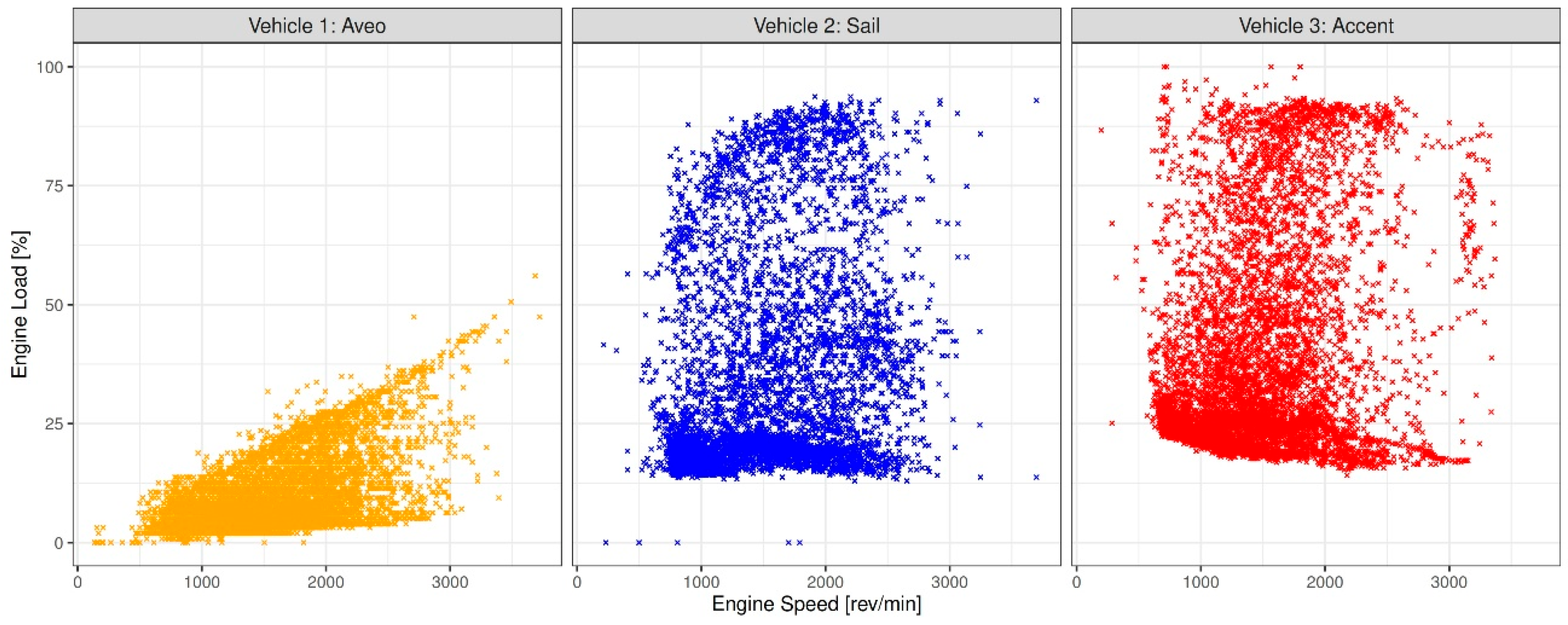
Figure 3 shows typical engine operating patterns of tested vehicles (Aveo, Sail, and Accent) regarding engine load versus engine speed. Each data point represents a second-by-second operating record for each car. In the case of Vehicle 1 (Aveo), depicted in orange, there is a clear positive correlation between engine speed and engine load, indicating that as engine speed increases, engine load also tends to increase. Most of the data for this vehicle are concentrated in engine load ranges below 25% and speed ranges under 2500 rev/min.

Figure 3.
Typical engine operation patterns by load and speed for tested vehicles.
In contrast, Vehicle 2 (Sail), depicted in blue, shows a broader distribution of data points across engine loads and speeds. This vehicle primarily operates in the 1000–2000 rpm range with engine loads between 12 and 30%. Finally, Vehicle 3 (Accent), shown in red, exhibits a similar trend to Vehicle 2 but with a slightly more dispersed pattern, suggesting more varied operating conditions.
Vehicle 1 (Aveo) exhibits a distinct engine load profile compared to the other two vehicles. Notably, when Vehicle 1 operates under idle conditions, its engine load is near zero, which contrasts sharply with Vehicles 2 and 3, which maintain an engine load of around 20% at idle. This variation at idle conditions highlights the relative nature of engine load, which can differ depending on the car manufacturer. According to the work in [25], assuming that engine load represents engine torque requires verifying the linearity between these two parameters using a chassis dynamometer. This verification is essential for accurately interpreting the engine load data. Furthermore, identifying the torque value under idle conditions is necessary to adjust the offset between engine load and torque parameters. Hence, the engine maps in this study are expressed in terms of engine load instead of torque.
4.2. Engine Maps Based on OBD Data
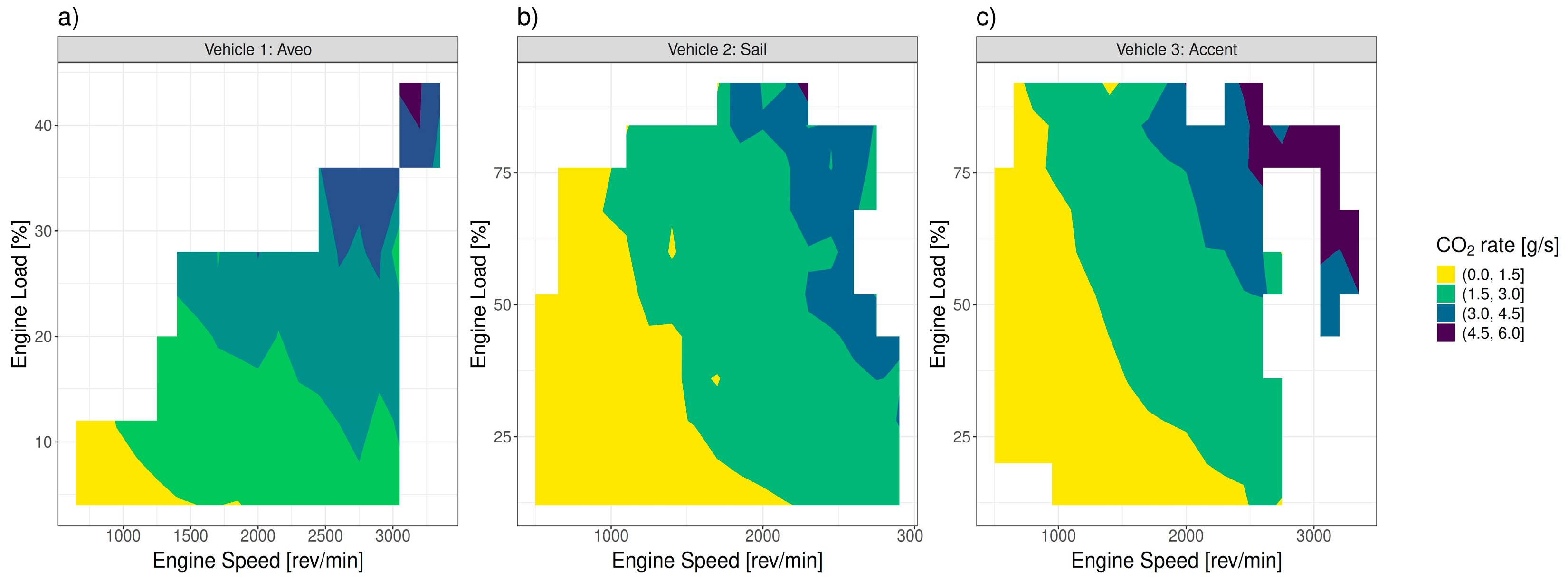
Figure 4 presents engine maps for the three tested vehicle engines, illustrating how the fuel consumption rate (measured in g/s, represented by a color gradient from yellow to blue) varies across different operational ranges. The three engine maps demonstrate that fuel consumption is proportional to engine load demand, reaching up to 2 g/s.

Figure 4.
Engine maps illustrating the CO2 emission rates for the Aveo (a), Sail (b) and Accent (c) vehicles.
For Vehicle 1, the engine primarily exhibits fuel consumption rates between 0.4 and 1.2 g/s in medium engine load and speed regions. During idling conditions common in urban driving, fuel consumption decreases to around 0.4 g/s (yellow). Vehicles 2 and 3 operate over more loads and speeds than Vehicle 1. Consequently, the engines from Vehicles 2 and 3 show a broader operational pattern, with significant zones in the medium fuel rate range (green and blue, 0.4–1.2 g/s). Additionally, these engines exhibit fuel rates near 0.4 g/s under idling conditions.
Overall, the engine maps indicate higher engine loads and speeds in average fuel consumption rates. Maximum fuel consumption rates can be up to five times higher than the minimum rates observed under idling conditions. The fuel consumption rates in this study align with those reported for light vehicles in China [35] over a decade ago. However, compared to more recent European studies [15,36], the observed fuel consumption rates are higher. This difference may be due to the lower engine technology of the vehicles evaluated. Furthermore, many modern vehicles in Latin America are often equipped with older technologies, contributing to increased fuel consumption rates.
4.3. Comparative Analysis Based on Vehicle-Specific Power
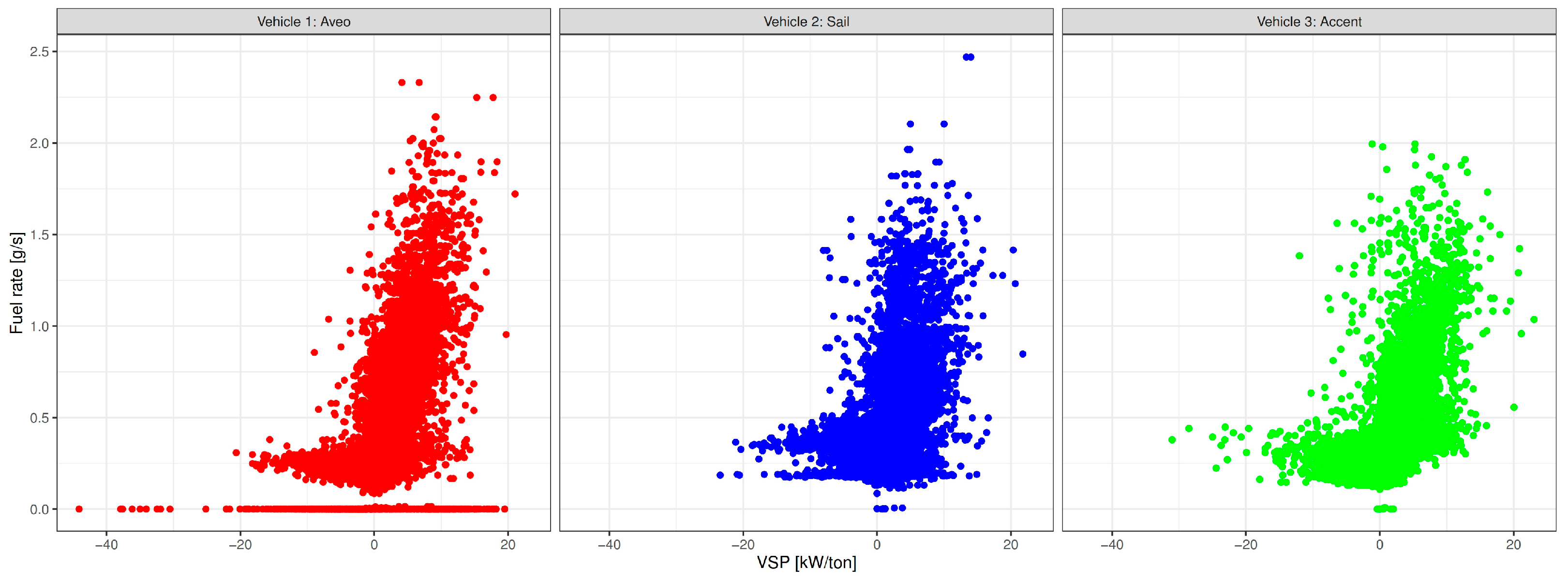
Figure 5 illustrates the correlation between instantaneous VSP values and the fuel consumption rate for the tested vehicles. In this graph, each point represents a vehicle operation record captured second by second. As previously mentioned, VSP is an energy-based variable that accounts for the vehicle’s tractive power and mass, enabling an absolute comparison of vehicle performance.
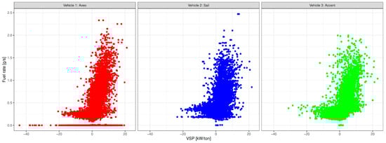
Figure 5.
Correlation between fuel rate and VSP for tested vehicles.
Overall, Figure 5 shows a general increasing trend for all three vehicles, indicating that as VSP rises, the fuel consumption rate increases. Vehicle 1 exhibits a slightly broader distribution of data points compared to Vehicles 2 and 3, with a notably higher number of points near fuel rates close to 0 g/s. These records indicate fuel cut-off conditions and may correspond to more efficient engine control module (ECM) management during downhill or deceleration events.
The observed increasing trends based on VSP are consistent with findings from previous studies on light-duty vehicles [35,37] and buses [6,33]. This further validates using VSP as a critical indicator for analyzing, comparing, and characterizing vehicle fuel consumption patterns. Consequently, VSP was highly useful in developing emission models, such as the Motor Vehicle Emission Simulator (MOVES) developed by the United States Environmental Protection Agency (EPA) [38] and COPERT (Computer Programme to Calculate Emissions from Road Transport) in Europe [39]. However, the application of VSP in Latin America was limited to a few previous studies conducted in Mexico [7] and Colombia [5].
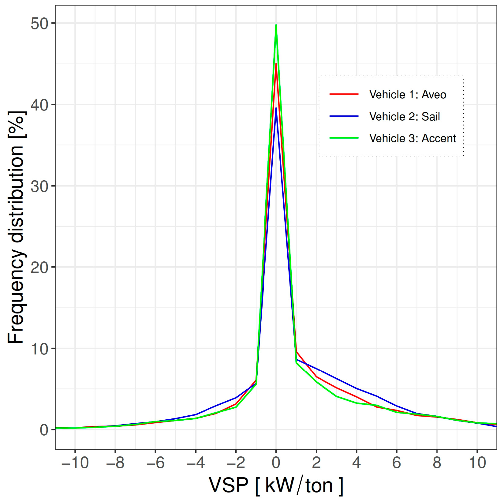
Figure 6 presents the VSP frequency distribution for tested vehicles, highlighting distinct operational differences. Vehicle 3 (green) shows the highest peak frequency, followed by Vehicle 2 (blue) and Vehicle 1 (red), suggesting that Vehicle 3 spends more time idling than the others. As VSP values shift into the negative range, indicating deceleration or downhill slopes, the frequency distribution gradually decreases for all vehicles. Vehicle 2 (blue) exhibits a slightly higher frequency in these harmful bins, implying that it operates during more extended periods while decelerating or descending compared to Vehicles 1 and 3.
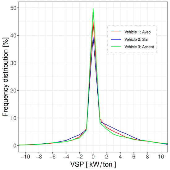
Figure 6.
VSP frequency distribution for tested vehicles.
In the positive VSP range, which corresponds to acceleration or an increased power demand, the frequency distribution sharply declines for all vehicles. While Vehicles 1 (red) and 2 (blue) display similar trends, Vehicle 3 (green) exhibits a slightly higher frequency, indicating that it spends more time accelerating or under higher power demands. These trends underscore the operational differences, with Vehicle 3 more frequently idling and accelerating, while Vehicle 2 has a greater tendency for deceleration.
All three vehicles show frequency distributions more significant than 38% for VSP values near zero, primarily reflecting idling conditions. This finding aligns with their primary use as taxis in urban environments and is consistent with previous studies reporting similar VSP values for taxis under idling conditions [37,40,41].
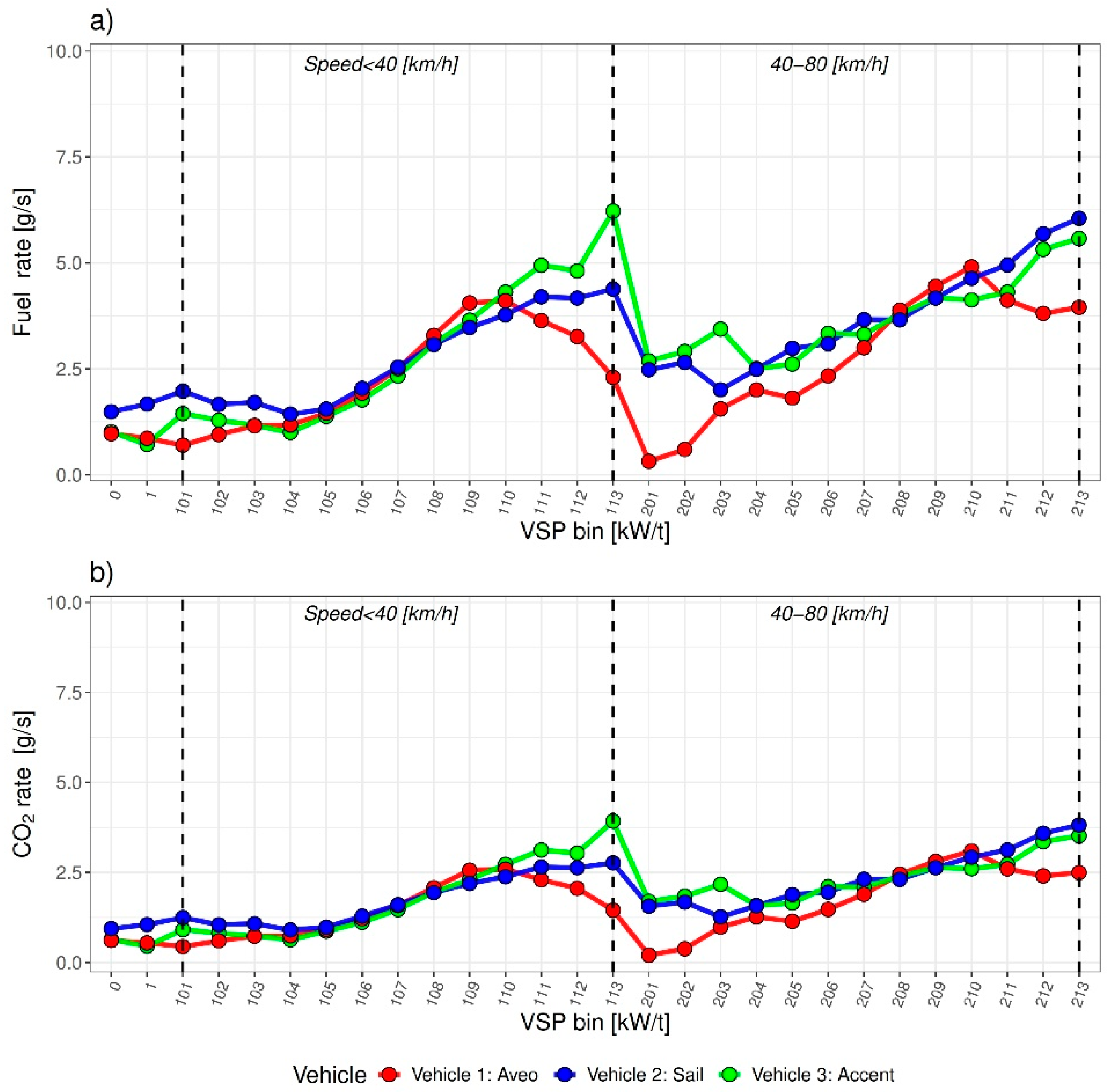
Figure 7a,b provide a comparative analysis of fuel consumption rate and CO2 emission rate, respectively, as functions of VSP bins for the tested vehicles. The VSP mode bins were defined by combining VSP and vehicle speed, as detailed in the Methodology section. Distinct patterns emerge when examining the trends across different speed intervals.
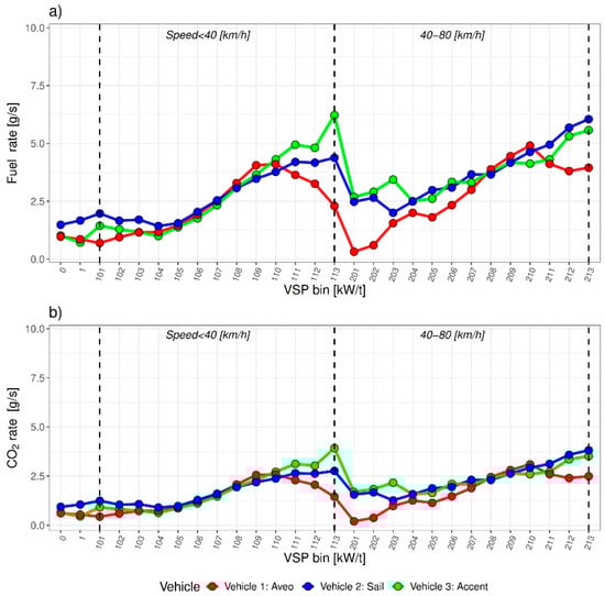
Figure 7.
Fuel emission rate (a) and CO2 emission rate (b) by VSP bin for tested vehicles.
Under idling and deceleration conditions (bins 0 and 1), Vehicle 3 consistently exhibited higher fuel consumption and CO2 emissions than the other vehicles, indicating lower engine efficiency even under minimal load conditions. For speeds below 40 km/h, both Vehicle 2 and Vehicle 3 displayed pronounced peaks in fuel consumption and CO2 emissions at VSP bin 113, corresponding to a high-load operating condition. In contrast, Vehicle 1 maintained significantly lower rates throughout this speed range.
Within the 40–80 km/h range, Vehicle 2 showed increased fuel consumption and CO2 emissions as VSP increased, while Vehicle 3 demonstrated a more moderate response. Vehicle 1 continued to exhibit the most efficient performance. Vehicle 1 consistently displayed lower fuel consumption across all VSP bins, particularly at lower speeds. Conversely, Vehicle 3 demonstrated a higher sensitivity to VSP variations.
These findings underscore the critical influence of vehicle design and engine efficiency on fuel consumption and emissions under diverse driving conditions. Moreover, the data presented in Figure 7a,b provide essential insights for developing an accurate energy-based emissions model. Notably, this study’s fuel consumption and CO2 emissions rates are higher than those reported in previous studies based on VSP bins [3,40]. These discrepancies may be attributed to the older engine technologies prevalent in vehicles marketed in Latin America, as discussed previously.
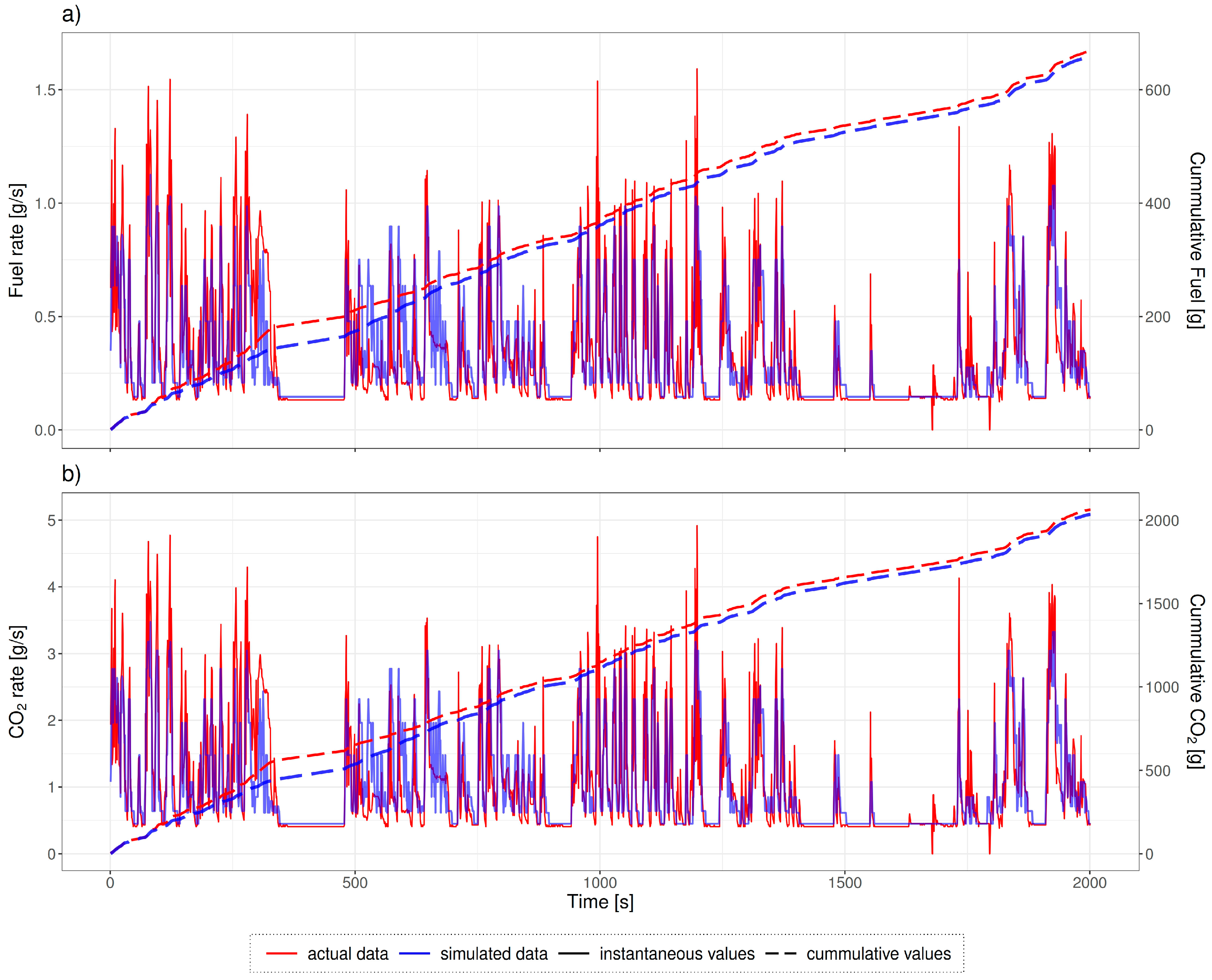
4.4. Performance of the VSP-Based Emission Model
Figure 8a,b present an example of a travel section for K iteration, comparing actual data (red) and VSP-simulated data (blue) for fuel consumption (Figure 8a) and CO2 emissions (Figure 8b) of Vehicle 3. The continuous lines represent second-by-second instantaneous values, while the dashed lines compare the cumulative values over time. In both figures, the actual and simulated data follow similar trends, indicating reasonable accuracy of the simulation model in capturing the dynamic behavior of fuel consumption and CO2 emissions. However, some discrepancies are noticeable.
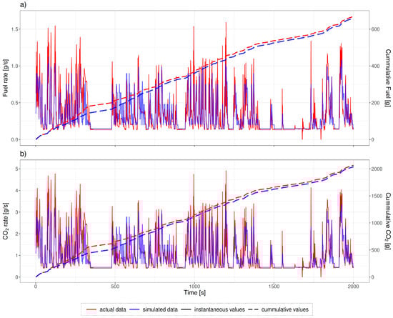
Figure 8.
Comparison of measured and simulated data using the VSP model for a typical trip of the Hyundai Accent vehicle: (a) Fuel consumption and (b) CO2 emissions.
The actual data show more significant variability and higher peaks, suggesting that the real driving conditions introduce more fluctuations than those captured by the simulation. For cumulative values, fuel consumption and CO2 emissions exhibit closely matching trends between actual and simulated data, although the simulated values tend to underestimate the actual cumulative totals slightly. This underestimation implies that, although the simulation model effectively captures overall trends, further refinement is necessary to better account for the higher variability observed under real-world conditions. Figure 8a,b demonstrate that VSP model simulations provide a valuable approximation of vehicle fuel consumption and emissions.
Table 6 presents a comparative analysis of the validation results for a VSP-based model applied to the three tested vehicles. The VSP model is validated using the k-fold-cross-validation approach, focusing on three metrics: relative error, Pearson correlation, and Root Mean Squared Error (RMSE) for fuel consumption and CO2 emissions. The model demonstrates a robust predictive accuracy across all three vehicles, with relatively low relative errors and moderate to high correlation coefficients. When comparing actual and predicted cumulative values for fuel consumption and CO2 emissions, the relative errors are below 3%. These results align with those reported in other VSP-based model simulations for light-duty vehicles [37,42], trucks [43], and buses [6], which typically report errors in the range of 4–8%.
Table 6.
Overview of the validation model from iterations for FC and CO2 emissions for tested vehicles.
The proposed VSP-based model exhibits an acceptable correlation for second-by-second data, with Pearson correlation coefficients ranging from 60% to 80% and reasonable RMSE values. A notable advantage of this VSP-based model, developed using OBD data, is its capability to predict second-by-second fuel consumption and CO2 emissions at a microscopic level, provided that speed profiles, driving cycles, or VSP distributions are available. This approach is particularly relevant for Latin America, where the use of some emission models, such as the ‘Passenger Car and Heavy Duty Emission Model’ (PHEM) and the ‘Motor Vehicle Emissions Simulator’ (MOVES), developed in different spatial domains like Europe or North America, may result in significant discrepancies in estimated emissions for Latin American cities due to differing driving patterns, emission data, and congestion levels [5]. Consequently, the VSP-based model offers a valuable and contextually appropriate tool for predicting emissions in Latin America, making it a crucial asset for regional environmental assessment and policy development.
4.5. Overview of Vehicle Performance Based on OBD Data
Table 7 provides a comprehensive overview of the engine performance characteristics for tested vehicles, focusing on metrics such as VSP, fuel consumption and CO2 emission rates, and both distance-based and energy-based emission factors. Several vital trends emerge when comparing the three vehicles. Vehicle 2 exhibits the highest VSP, indicating a greater power output than its weight. However, this increased power is accompanied by slightly higher fuel consumption and CO2 emissions than Vehicles 1 and 3. Conversely, Vehicle 3 demonstrates the lowest VSP and fuel consumption and CO2 emissions when considering energy-based emission factors, suggesting a more fuel-efficient design.
Table 7.
Overall engine performance of fuel efficiency, energy emissions, emission rates, and distance emissions by vehicle.
Regarding distance-based emission factors, Vehicle 1 shows the lowest fuel consumption and CO2 emissions, while Vehicle 3 presents the highest values. Notably, despite Vehicle 2’s higher VSP, its distance-based and energy-based emission factors are not proportionally elevated, indicating that a higher power output does not necessarily translate to higher emissions per unit of distance or energy.
The distance-based CO2 emission factors identified (249–260 g CO2/km), which predominantly reflect full urban operating conditions of LDVs in Latin America, are consistent with results reported for gasoline taxis in China [44] with values around 230 g CO2/km. However, the CO2 emission factors observed in this study are significantly higher than those reported in previous studies [3,40] for light-duty gasoline vehicles, including urban, suburban, and motorway sections, with values ranging from 130 to 190 g CO2/km. This discrepancy may be attributed to differences in vehicle technology, driving patterns, and the specific urban conditions of this study.
5. Conclusions and Future Work
This study demonstrates the feasibility of using low-cost OBD data to develop detailed engine maps and analyze urban taxis’ fuel efficiency and CO2 emissions under real-world driving conditions. The proposed methodology, which combines a VSP analysis with OBD-collected data, enables a detailed assessment of vehicles without the need for more expensive equipment like PEMS.
The results confirm that the OBD-based approach can effectively monitor vehicle performance in real-world urban traffic conditions, providing valuable insights for improving the sustainability of urban transport. Furthermore, the methodology is advantageous in regions like Latin America, where access to advanced equipment such as PEMS is limited. However, while the method captures general trends, cumulative fuel consumption and CO2 emissions are slightly underestimated. This suggests that the model could be refined to better account for the fluctuations observed in real-world conditions.
The implications of these findings are significant for urban transportation policies, especially in resource-constrained regions such as Latin America. The demonstrated feasibility of using low-cost OBD data provides a practical solution that can support policymakers in several key areas: (i) improving the accuracy of local emissions inventories, (ii) establishing more region-specific emission control regulations based on local geography and vehicle fleet characteristics, (iii) encouraging the renewal of fuel-inefficient vehicle fleets, and (iv) more effectively targeting fuel subsidies.
In the future, it is recommended that this methodology be extended to other vehicle categories and geographic areas to validate its broader applicability. Additionally, integrating advanced techniques such as machine learning could significantly improve the model’s predictive accuracy. A direct comparison with other methodologies, such as those based on PEMS, would also be valuable in further validating the precision and utility of this approach in a vehicle emission assessment. These potential avenues for future improvements make the future of this research attractive.
While this study introduces an innovative, low-cost method for assessing vehicle performance using OBD data and mobile technology, it has limitations. A fundamental limitation is the inability to directly validate fuel consumption estimates from the OBD interface with actual vehicle fuel consumption. Future research should address this by comparing OBD estimates with precise fuel measurements obtained through flowmeters, ensuring a more accurate assessment of vehicle performance and emissions in real-world conditions.
Author Contributions
This paper was a collaborative effort among all authors. All authors participated in the analysis, discussed the results, and wrote the paper. All authors have read and agreed to the published version of the manuscript.
Funding
This research was funded by the Universidad Técnica del Norte, within the project 0000001223.
Data Availability Statement
The original contributions presented in the study are included in the article, further inquiries can be directed to the corresponding author.
Conflicts of Interest
The authors declare no conflicts of interest.
References
- Frey, H.C. Trends in Onroad Transportation Energy and Emissions. J. Air Waste Manag. Assoc. 2018, 68, 514–563. [Google Scholar] [CrossRef] [PubMed]
- Blanco Bonilla, A.; Ejecutivo, S.; Castillo, T.; García, F.; Mosquera, L.; Rivadeneira, T.; Segura, K.; Yujato, M.; Gain, K.; Guerra, L.; et al. Panorama Energético de Amaérica Latina El El Caribe 2022; Olade: Quito, Ecuador, 2022. [Google Scholar]
- Yuan, W.; Frey, H.C.; Wei, T.; Rastogi, N.; VanderGriend, S.; Miller, D.; Mattison, L. Comparison of Real-World Vehicle Fuel Use and Tailpipe Emissions for Gasoline-Ethanol Fuel Blends. Fuel 2019, 249, 352–364. [Google Scholar] [CrossRef]
- Gallus, J.; Kirchner, U.; Vogt, R.; Benter, T. Impact of Driving Style and Road Grade on Gaseous Exhaust Emissions of Passenger Vehicles Measured by a Portable Emission Measurement System (PEMS). Transp. Res. Part D Transp. Environ. 2017, 52, 215–226. [Google Scholar] [CrossRef]
- Rodríguez, R.A.; Virguez, E.A.; Rodríguez, P.A.; Behrentz, E. Influence of Driving Patterns on Vehicle Emissions: A Case Study for Latin American Cities. Transp. Res. Part D Transp. Environ. 2016, 43, 192–206. [Google Scholar] [CrossRef]
- Rosero, F.; Fonseca, N.; López, J.-M.; Casanova, J. Effects of Passenger Load, Road Grade, and Congestion Level on Real-World Fuel Consumption and Emissions from Compressed Natural Gas and Diesel Urban Buses. Appl. Energy 2021, 282, 116195. [Google Scholar] [CrossRef]
- Giraldo, M.; Huertas, J.I. Real Emissions, Driving Patterns and Fuel Consumption of in-Use Diesel Buses Operating at High Altitude. Transp. Res. Part D Transp. Environ. 2019, 77, 21–36. [Google Scholar] [CrossRef]
- EPA. Greenhouse Gas Emissions Standards and Fuel Efficiency Standards for Medium- and Heavy-Duty Engines and Vehicles; EPA: Washington, DC, USA, 2011; Volume 76. [Google Scholar]
- EPA; NHTSA; DOT. Greenhouse Gas Emissions and Fuel Efficiency Standards for Medium- Heavy-Duty Engines and Vehicles—Phase 2; EPA: Washington, DC, USA, 2016; Volume 81, pp. 73478–74274. [Google Scholar]
- EU Commission Regulation (EU) No 582/2011 of 25 May 2011 Implementing and Amending Regulation (EC) No 595/2009 of the European Parliament and of the Council with Respect to Emissions from Heavy Duty Vehicles (Euro VI) and Amending Annexes I and III to Direct. Available online: https://eur-lex.europa.eu/eli/reg/2011/582/oj (accessed on 14 May 2024).
- Luján, J.M.; Bermúdez, V.; Dolz, V.; Monsalve-Serrano, J. An Assessment of the Real-World Driving Gaseous Emissions from a Euro 6 Light-Duty Diesel Vehicle Using a Portable Emissions Measurement System (PEMS). Atmos. Environ. 2018, 174, 112–121. [Google Scholar] [CrossRef]
- European Commission and Council of the European Union Commission Regulation (EU) 2016/427 Amending Regulation (EC) No 692/2008 as Regards Emissions from Light Passenger and Commercial Vehicles (Euro 6) (Text with EEA Relevance). Off. J. Eur. Union 2016, 82, 1–98.
- EU. Commission Regultaion (EU) 2019/318 of 19 February 2019 Amending Regulation (EU) 2017/2400 and Directive 2007/46/EC of the European Parliament and of the Council as Regards the Determination of the CO2 Emissions and Fuel Consumption of Heavy-Duty Vehicle; European Union: Maastricht, The Netherlands, 2019; Volume 2011. [Google Scholar]
- Acevedo, H.; Delgado, O.; Pineda, L.; Pettigrew, S. Hoja De Ruta Para Descarbonizar El Transporte De Carga En América Latina Entre 2025 Y 2050. Atmos. Environ. 2023, 188, 1–30. [Google Scholar]
- Mera, Z.; Varella, R.; Baptista, P.; Duarte, G.; Rosero, F. Including Engine Data for Energy and Pollutants Assessment into the Vehicle Specific Power Methodology. Appl. Energy 2022, 311, 118690. [Google Scholar] [CrossRef]
- Kroyan, Y.; Wojcieszyk, M.; Kaario, O.; Larmi, M. Modelling the End-Use Performance of Alternative Fuel Properties in Flex-Fuel Vehicles. Energy Convers. Manag. 2022, 269, 116080. [Google Scholar] [CrossRef]
- Zhang, M.; Cheng, W.; Shen, Y. Designing Heavy-Duty Vehicles’ Four-Parameter Driving Cycles to Best Represent Engine Distribution Consistency. IEEE Access 2020, 8, 212079–212093. [Google Scholar] [CrossRef]
- He, L.; Hu, J.; Yang, L.; Li, Z.; Zheng, X.; Xie, S.; Zu, L.; Chen, J.; Li, Y.; Wu, Y. Science of the Total Environment Real-World Gaseous Emissions of High-Mileage Taxi Fl Eets in China. Sci. Total Environ. 2019, 659, 267–274. [Google Scholar] [CrossRef] [PubMed]
- Castresana, J.; Gabiña, G.; Martin, L.; Basterretxea, A.; Uriondo, Z. Marine Diesel Engine ANN Modelling with Multiple Output for Complete Engine Performance Map. Fuel 2022, 319, 123873. [Google Scholar] [CrossRef]
- Dekraker, P.; Barba, D.; Moskalik, A.; Butters, K. Constructing Engine Maps for Full Vehicle Simulation Modeling. SAE Technol. Pap. Ser. 2018, 1, 4. [Google Scholar] [CrossRef]
- Acevedo, H.; Delgado, O. Mecanismos de Bajo Costo Para La Verificación y Control de Emisiones Vehiculares En Colombia. 2023. Available online: https://theicct.org/wp-content/uploads/2023/05/heavy-vehicles-Colombia-costs-may23.pdf (accessed on 10 March 2024).
- Sierra, J.C. Estimating Road Transport Fuel Consumption in Ecuador. Energy Policy 2016, 92, 359–368. [Google Scholar] [CrossRef]
- EPA. EPA Finalizes Regulations Requiring Onboard Diagnostic Systems on 2010 and Later Heavy-Duty Engines Used in Highway Applications Over 14,000 Pounds; Revisions to Onboard Diagnostic Requirements for Diesel Highway Heavy-Duty Applications Under 14,000 Pound; EPA: Washington, DC, USA, 2008. [Google Scholar]
- Horiba. On Board Emission Measurement System OBS-2200 Instruction Manual. 2006. Available online: https://www.horiba.com/int/automotive/products/detail/action/show/Product/obs-one-gs-unit-28/ (accessed on 22 June 2024).
- Alessandrini, A.; Filippi, F.; Ortenzi, F. Consumption Calculation of Vehicles Using OBD Data. 2012 Int. Emiss. Invent. Conf. “Emission Invent.—Meet. Challenges Posed by Emerg. Glob. Natl. Reg. Local Air Qual. Issues” 2012, 1–21. Available online: https://static.horiba.com/fileadmin/Horiba/Products/Automotive/Emission_Measurement_Systems/OBS-ONE/OBS-ONE_Brochure_English.pdf (accessed on 25 March 2024).
- Posada, F.; Bandivadekar, A. Global Overview of On-Board Diagnostic (OBD) Systems for Heavy-Duty Vehicles [White Paper]; 2015. Available online: https://theicct.org/wp-content/uploads/2021/06/ICCT_Overview_OBD-HDVs_20150209.pdf (accessed on 3 March 2024).
- Instituto de Investigación Geológico y Energético de Ecuador. Balance Energético Nacional Del Ecuador 2021; Instituto de Investigación Geológico y Energético de Ecuador: Quito, Ecuador, 2022. [Google Scholar]
- European Commission. Commission Regulation (EU) 2017/1151 of 1 June 2017 Supplementing Regulation (EC) No 715/2007 of the European Parliament and of the Council on Type-Approval of Motor Vehicles with Respect to Emissions from Light Passenger and Commercial Vehicles (Euro 5 A). Off. J. Eur. Union 2017, 1–643. Available online: https://eur-lex.europa.eu/legal-content/EN/TXT/PDF/?uri=CELEX:32007R0715 (accessed on 15 January 2024).
- Rosero, F.; Fonseca, N.; López, J.-M.J.-M.; Casanova, J. Real-World Fuel Efficiency and Emissions from an Urban Diesel Bus Engine under Transient Operating Conditions. Appl. Energy 2020, 261, 114442. [Google Scholar] [CrossRef]
- RStudio. RStudio Desktop. Available online: https://s3.amazonaws.com/rstudio-ide-build/electron/windows/RStudio-2023.09.0-463.exe (accessed on 26 January 2024).
- Wickham, H. Ggplot2: Elegant Graphics for Data Analysis; Tidiverse, Ed.; Springer: New York, NY, USA, 2016; ISBN 978-3-319-24277-4. [Google Scholar]
- Jiménez-Palacios, J.L. Understanding and Quantifying Motor Vehicle Emissions with Vehicle Specific Power and TILDAS Remote Sensing. Ph.D. Thesis, Massachusetts Institute of Technology (MIT), Cambridge, MA, USA, 1999. [Google Scholar]
- Zhai, H.; Frey, H.C.; Rouphail, N.M. A Vehicle-Specific Power Approach to Speed- and Facility-Specific Emissions Estimates for Diesel Transit Buses. Environ. Sci. Technol. 2008, 42, 7985–7991. [Google Scholar] [CrossRef]
- Alves, J.; Baptista, P.C.; Gonçalves, G.A.; Duarte, G.O. Indirect Methodologies to Estimate Energy Use in Vehicles: Application to Battery Electric Vehicles. Energy Convers. Manag. 2016, 124, 116–129. [Google Scholar] [CrossRef]
- Song, G.; Yu, L. Estimation of Fuel Efficiency of Road Traffic by Characterization of Vehicle-Specific Power and Speed Based on Floating Car Data. Transp. Res. Rec. J. Transp. Res. Board 2009, 2139, 11–20. [Google Scholar] [CrossRef]
- Bishop, J.D.K.; Stettler, M.E.J.; Molden, N.; Boies, A.M. Engine Maps of Fuel Use and Emissions from Transient Driving Cycles. Appl. Energy 2016, 183, 202–217. [Google Scholar] [CrossRef]
- He, W.; Duan, L.; Zhang, Z.; Zhao, X.; Cheng, Y. Analysis of the Characteristics of Real-World Emission Factors and VSP Distributions—A Case Study in Beijing. Sustainability 2022, 14, 11512. [Google Scholar] [CrossRef]
- EPA. Exhaust Emission Rates for Heavy—Duty On—Road Vehicles in MOVES2014 Exhaust Emission Rates for Heavy—Duty On—Road Vehicles in MOVES2014; EPA: Washington, DC, USA, 2015. [Google Scholar]
- Li, F.; Zhuang, J.; Cheng, X.; Li, M.; Wang, J.; Yan, Z. Investigation and Prediction of Heavy-Duty Diesel Passenger Bus Emissions in Hainan Using a COPERT Model. Atmosphere 2019, 10, 106. [Google Scholar] [CrossRef]
- Yao, Z.; Cao, X.; Shen, X.; Zhang, Y.; Wang, X.; He, K. On-Road Emission Characteristics of CNG-Fueled Bi-Fuel Taxis. Atmos. Environ. 2014, 94, 198–204. [Google Scholar] [CrossRef]
- Ghaffarpasand, O.; Talaie, M.R.; Ahmadikia, H.; TalaieKhozani, A.; Shalamzari, M.D.; Majidi, S. On-Road Performance and Emission Characteristics of CNG-Gasoline Bi-Fuel Taxis/Private Cars at the Roadside Environment. Atmos. Pollut. Res. 2020, 11, 1743–1753. [Google Scholar] [CrossRef]
- Zhai, Z.; Song, G.; Yu, L. How Much Vehicle Activity Data Is Needed to Develop Robust Vehicle Specific Power Distributions for Emission Estimates? A Case Study in Beijing. Transp. Res. Part D Transp. Environ. 2018, 65, 540–550. [Google Scholar] [CrossRef]
- Zhang, S.; Yu, L.; Song, G. Emissions Characteristics for Heavy-Duty Diesel Trucks Under Different Loads Based on Vehicle-Specific Power. Transp. Res. Rec. J. Transp. Res. Board 2017, 2627, 77–85. [Google Scholar] [CrossRef]
- Hu, J.; Wu, Y.; Wang, Z.; Li, Z.; Zhou, Y.; Wang, H.; Bao, X.; Hao, J. Real-World Fuel Efficiency and Exhaust Emissions of Light-Duty Diesel Vehicles and Their Correlation with Road Conditions. J. Environ. Sci. 2012, 24, 865–874. [Google Scholar] [CrossRef]
Disclaimer/Publisher’s Note: The statements, opinions and data contained in all publications are solely those of the individual author(s) and contributor(s) and not of MDPI and/or the editor(s). MDPI and/or the editor(s) disclaim responsibility for any injury to people or property resulting from any ideas, methods, instructions or products referred to in the content. |
© 2024 by the authors. Licensee MDPI, Basel, Switzerland. This article is an open access article distributed under the terms and conditions of the Creative Commons Attribution (CC BY) license (https://creativecommons.org/licenses/by/4.0/).