Comprehensive Comparison of Physical and Behavioral Approaches for Virtual Prototyping and Accurate Modeling of Three-Phase EMI Filters

Abstract

This paper addresses and compares the modeling of typical EMI filters used in three-phase power equipment obtained through two different approaches, namely, physical and behavioral. Firstly, an innovative physical EMI filter modeling procedure is presented, which relies on an analytical formulation in terms of chain-parameters matrices and allows for an easy evaluation of its attenuation characteristics. The considered procedure builds an overall filter model by combining simple components models, requiring the determination of only a limited number of parasitic elements. Furthermore, the latter can be easily estimated without the need to build any prototype, avoiding the costly trial-and-error design procedures currently applied in the industrial context. Additionally, the considered physical model is tailored for high-power filters, built with thick wires, while most of the physical models available in the literature are aimed at small-sized filters built on printed circuit boards. The procedure is validated step by step, discussing the accuracy of each component model and its impact on overall accuracy compared to the actual measurements of the final assembled filter. Secondly, a behavioral modeling procedure is presented, which is based on external measurements performed on the filter prototype and provides an equivalent circuit model. Specifically, it extends to three-phase filters a circuit model previously developed for the single-phase case. Lastly, a critical comparison between the proposed physical and behavioral models is presented, highlighting the strengths and limitations of both and suggesting optimal uses for each.

1. Introduction

The prediction of conducted emissions (CE) generated by electronic power converters is of increasing interest for electromagnetic compatibility (EMC) specialists involved in product development, as traditional trial-and-error approaches imply significant costs, which could be greatly reduced by moving the design stage from laboratory activities to virtual environments. In these regards, circuit and electromagnetic simulation tools are promising for virtual prototyping, yet their fruitful use relies on the availability of suitable models of all the components included in the system under consideration.

CE can be evaluated both in time and frequency domains, as discussed in [1] and [2], respectively. However, both approaches exhibit advantages as well as limitations. Frequency domain modeling techniques are the most widely used, as they are directly related to concepts and prescriptions from EMC standards. Additionally, frequency-domain simulations are usually much less time-consuming than time-domain methods. Frequency-domain models are often behavioral models obtained by experimental measurements, and consist of impedances and sources as discussed in [3,4] for power electronics converters and related electrical equipment. Behavioral models are simple and accurate and are suitable for the analysis of CE in complex systems by frequency-domain simulation, yet they are not suitable to evaluate non-linear and/or time-variant systems, commonly observed in electronic power converters.

Conversely, the simulation of non-linear and/or time-variant systems is easily achieved by time-domain methods, at the expense of increased computational costs and model complexity. This is due to the fact that non-linear and or time-varying elements require detailed component-level circuit models, including parasitic elements [5], which can be inferred by 3D electromagnetic simulations [6] or impedance measurements [7]. A common example of such systems is represented by electronic power converters, the design [8,9] and control algorithms [10] of which often include modulation strategies purposefully designed to affect their CE.

EMI filters are widely used to mitigate CE, either as an integral part of equipment or as stand-alone products for complex systems [11]. For the latter case in particular, the design and selection of the optimal EMI filter for a given application are two significant tasks where the simulation of CE represents a great opportunity in industrial applications [12,13]. However, the requirements of filter modeling techniques for design or selection purposes are largely different. Indeed, for EMI filter design, the model is required to be built upon the knowledge of single filter components in order to obtain useful insights on how each component affects the overall filter performance, hence enabling the virtual prototyping of EMI filters. Unfortunately, the accuracy expected from this modeling approach is often limited to over a few tens of MHz, so it is not the best option for filter selection, i.e., when the main interest is to accurately evaluate which one among many filters is best suited to a particular application. In this case, the higher accuracy granted by behavioral models is required, at the expense of losing any insight on the relations between the overall filter performance and its internal components.

As regards the information necessary to define circuit models, little can usually be deduced from the technical data sheets of commercial products, which mostly provide the inner topology (with ideal component values) and attenuation plots, obtained experimentally for the Common-Mode (CM) and Differential-Mode (DM) according to the CISPR 17 standard [14]. Unfortunately, ideal values are of little help in predicting the filter performance as, above a few tens of kHz, the non-ideal behavior of the components (parasitic resistances, capacitances, and inductances) and the interconnects play a significant role [15,16]. Additionally, capacitive and inductive couplings may affect the performance of components which are close to each other [15]. Basic circuit models can be improved by adding parasitic elements, as discussed in [16] for the small construction of filters on printed circuit boards (PCBs); however, this option can be difficult to apply to filters intended for high-power converters whose geometry comprises some uncontrolled randomness (e.g., hand-made wired interconnects and windings). The model can be further improved, in principle, by using full-wave electromagnetic simulations to refine parasitic components values, as discussed in [17,18]. However, the limitations in the management of uncontrolled geometries related to the use of wire conductors instead of PCBs still hold.

Despite their limitations in terms of accuracy, this family of physical models can be fruitfully used during the filter design phase, as they can provide useful insights about how acting on single components alters the overall filter performance. A number of EMI filter design procedures are indeed available in the literature, which usually start from the analysis of the CE propagation path and, on this basis, suggest a possible filter topology and some components nominal values to meet CE requirements. As an example, in [19], the design of two different filter topologies for a SiC inverter is discussed. Similarly, in [20], two different, complementary filter design approaches for automotive converters are presented, while in [21], the principles of EMI filter design in avionic vehicular systems are analyzed based on a detailed model of CM and DM noise paths. Additionally, in [22], an optimal filter design method based on matching the considered converter source impedance is presented. The filter models used in these works, however, are not explicitly validated, as only final results based on experimental tests are reported. Additionally, as for most EMI filter models available in the literature, the aforementioned works address small-sized filters constructed on PCBs, whose geometry and parasitic effects are well controlled. A further step toward virtual prototyping is presented in [23], where a simulation-based filter design method is presented, providing good results despite using simple circuit models. However, in this case too, the used filter models are not explicitly validated, and only final results based on experimental tests are reported.

In summary, the physical modeling procedures available in the literature exhibit three main drawbacks. First, most contributions are intended to provide an accurate representation of an existing filter, which is achieved by augmenting the ideal circuit with a number of parasitic elements. However, since this approach relies on the availability of an already constructed filter, it is not suitable for virtual prototyping. Second, most of the literature contributions are targeted to small PCBs with controlled geometry and are not trivially scalable to high-power, three-phase filters, which are physically large and constructed by thick wires, thus characterized by inherent randomness. Third, physical models available in the literature are not explicitly validated step by step, so they do not evaluate the accuracy of each component model and its impact on the overall accuracy after integration in the final filter.

Regarding behavioral models, typical applications in the literature are time-domain circuit simulations that include time-varying and/or nonlinear components [24]. The recent contribution of [25] provides a robust, industrial solution for EMI filter modeling by a black-box modeling approach based on an external S-parameters characterization [26]. Specifically, the measured S-parameters are approximated by a rational function by means of the Vector Fitting algorithm [27,28,29] and passivity enforcement routines [30,31], and an equivalent circuit representation is built to make the model compatible with frequency- and time-domain SPICE simulations [32]. However, the modeling procedure discussed in [25] is developed for devices with four terminals, such as single-phase EMI filters, and has not been applied to a three-phase filter yet.

In order to overcome the aforementioned limitations of physical and behavioral modeling techniques, in this paper, two cutting-edge industrial procedures ascribed to physical and behavioral modeling approaches are introduced. The physical modeling approach relies on the inspection of the considered filter structure and of its components and builds an overall filter model by combining simple components models. This modeling approach lends itself to the virtual prototyping of the EMI filter, and is discussed in detail here, providing three main contributions with respect to the current state of the art:

(a)

The filter model relies on an analytical formulation in terms of chain-parameter matrices, which allows us to easily evaluate its attenuation characteristics. Furthermore, the model is designed to effectively predict filter behavior by including only a limited number of parasitic elements that can be easily estimated before any prototype is actually constructed (unlike previously discussed literature contributions).

(b)

The filter model is tailored for high-power filters, built with thick wires, while most physical model available in the literature are targeted toward small filters built on PCBs.

(c)

The physical model is validated step by step, discussing the accuracy of each component model and its impact on the overall filter model accuracy, and compared to measurements after the filter assembly.

Successively, a behavioral modeling methodology is applied to the filter prototype after production, which relies only on external measurements to determine an equivalent filter model. The considered behavioral modeling technique relies on a cutting-edge procedure available in the literature for single-phase filters only, which is here extended to correctly model three-phase filters.

Lastly, a comprehensive comparison between physical and behavioral approaches for virtual prototyping and the accurate modeling of EMI filters is presented, along with a detailed discussion of their applicability, accuracy, and best use.

This paper is structured as follows: Section 2 presents the considered filter design, and the available components on which to build the physical model. Section 3 discusses the considered physical EMI filter modeling procedure, while the considered behavioral EMI modeling procedure is presented in Section 4. Section 5 presents an extensive comparison of the two methods, highlighting their respective strengths and limitations, and, lastly, final conclusions and future research perspectives are reported in Section 6.

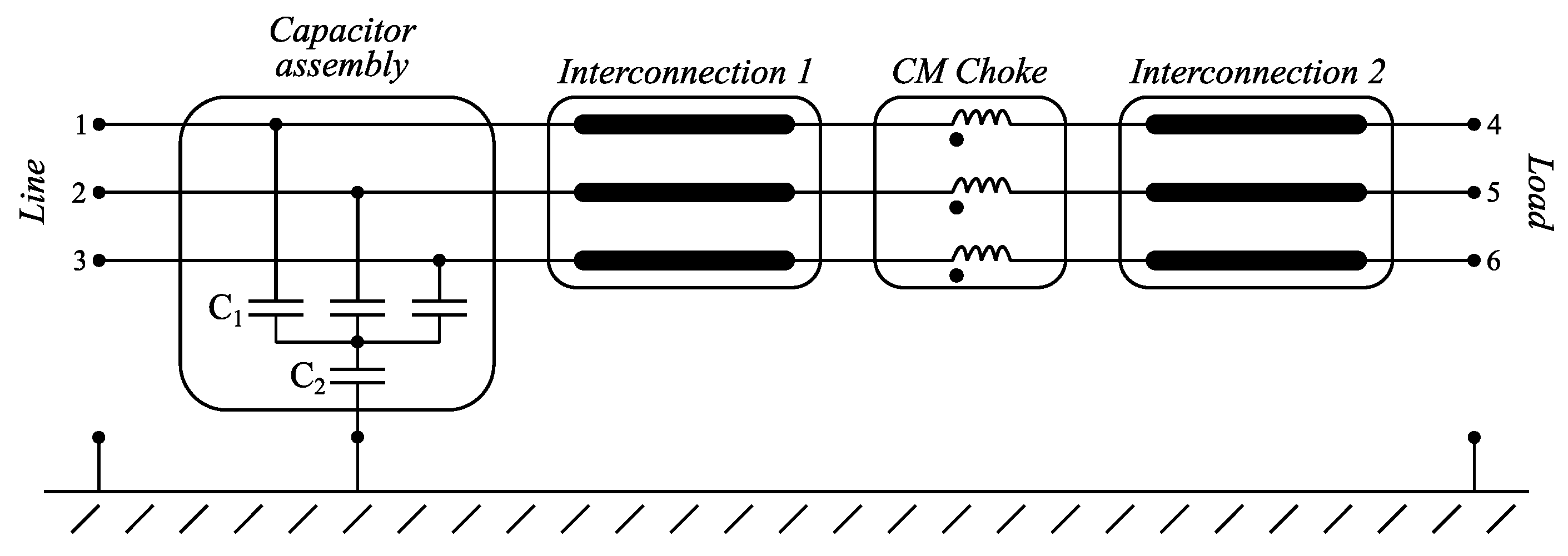
2. EMI Filter Example

With the aim of illustrating both a physical and behavioral modeling procedure, let us consider, with no loss of generality, a typical one-stage three-phase EMI filter, the block scheme of which is shown in Figure 1. As common practice for EMI filters required to withstand significant functional currents, the filter is built with single-core cables (and not on a PCB), enclosed in a metal box, and the CMC is wound using the same cables.

The filter prototype includes a capacitor assembly, realized with three, star-connected, 2200 nF capacitors (C₁), the star-center of which is connected to the metallic filter enclosure by means of a 100 nF capacitor (C₂). The filter also includes a CM choke (CMC), realized by single-core cables wound twice around a ferrite core. Sample 2200 nF and 100 nF capacitors, and one sample ferrite core selected for the realization of the CMC are reported in Figure 2. Lastly, two three-phase interconnections, which will be realized by common electrical single-core, PVC-insulated cables, link the CMC to the filter external terminals.

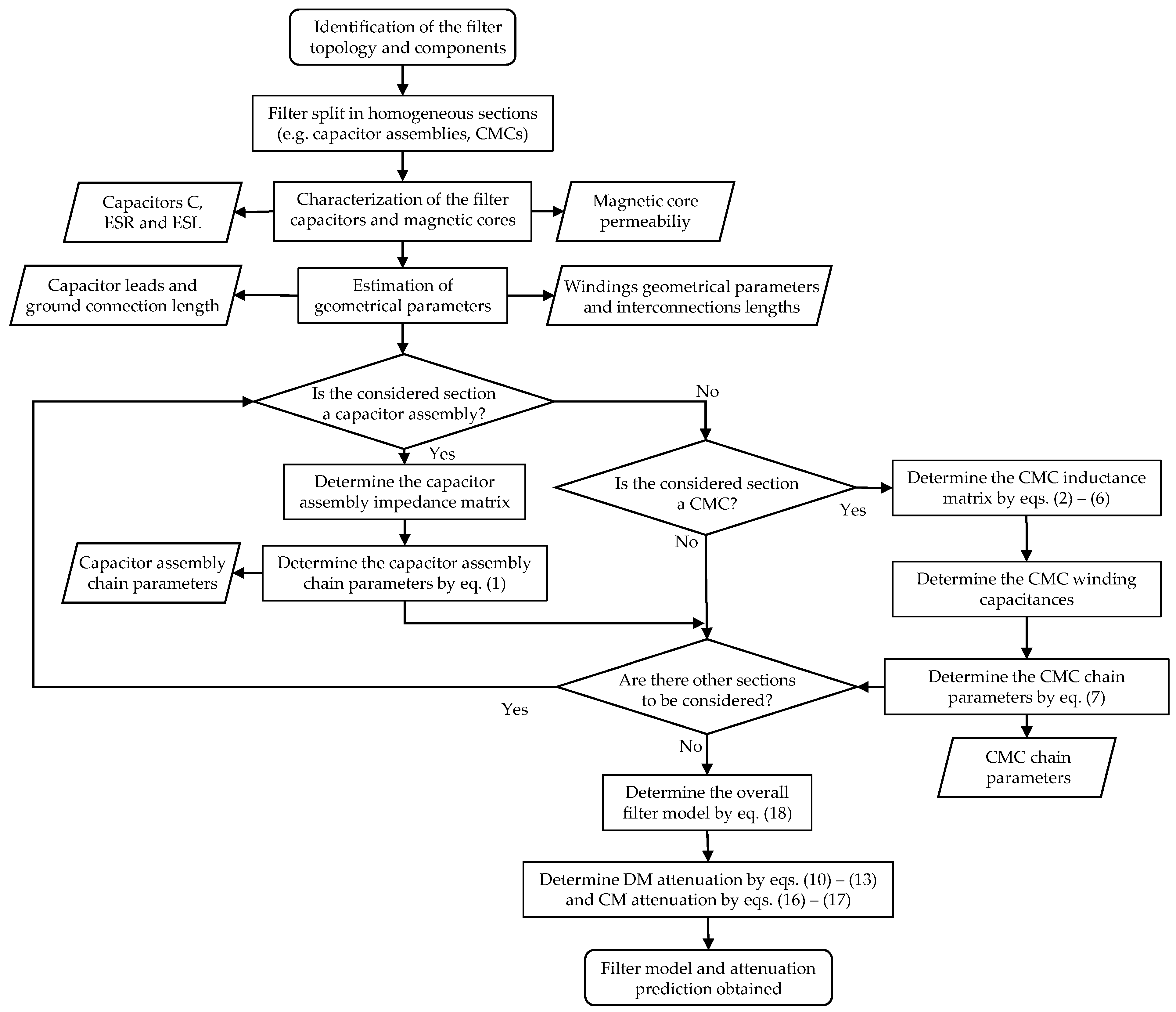
3. Physical Modeling Procedure for Three-Phase EMI Filters

The physical modeling approach is based on the knowledge of: (a) the filter structure, including circuit topology and known or estimated geometrical properties (cable lengths and position, etc.), and (b) the frequency response of each component included in the filter. Since typical EMI filters are realized by different components or groups of (e.g., assembly of capacitors between phases and/or to ground, common mode chokes, etc.), it is convenient to represent each of those in terms of its chain-parameter matrix, so that the overall filter chain-parameter matrix can be simply obtained by the product of the matrices representing each section. This approach introduces some level of approximation, as its underlying assumption is that no coupling between filter sections is present. However, it will be shown that it is still possible to obtain an acceptable level of accuracy for virtual prototyping purposes.

In the following, we will consider, with no loss of generality, the components appearing in the EMI filter prototype depicted in Figure 1, namely, capacitors assemblies, CMCs, and cable interconnections. Other possible (non-standard) occurrences may be treated analogously. Successively, we will show the results of the combination of each of the obtained models in the overall EMI filter model and compare the results with measurements performed on a filter prototype.

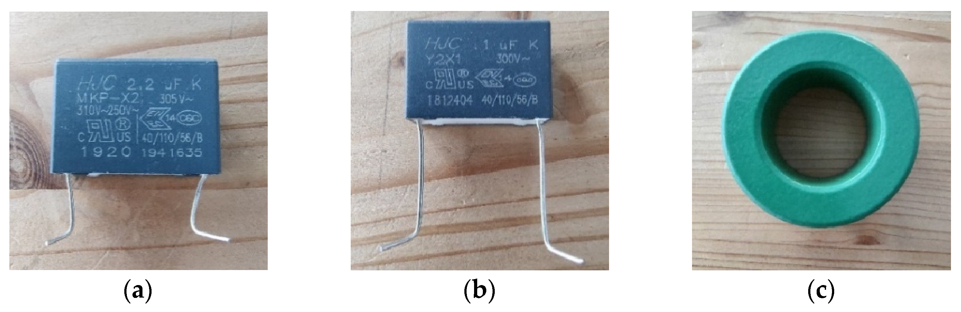
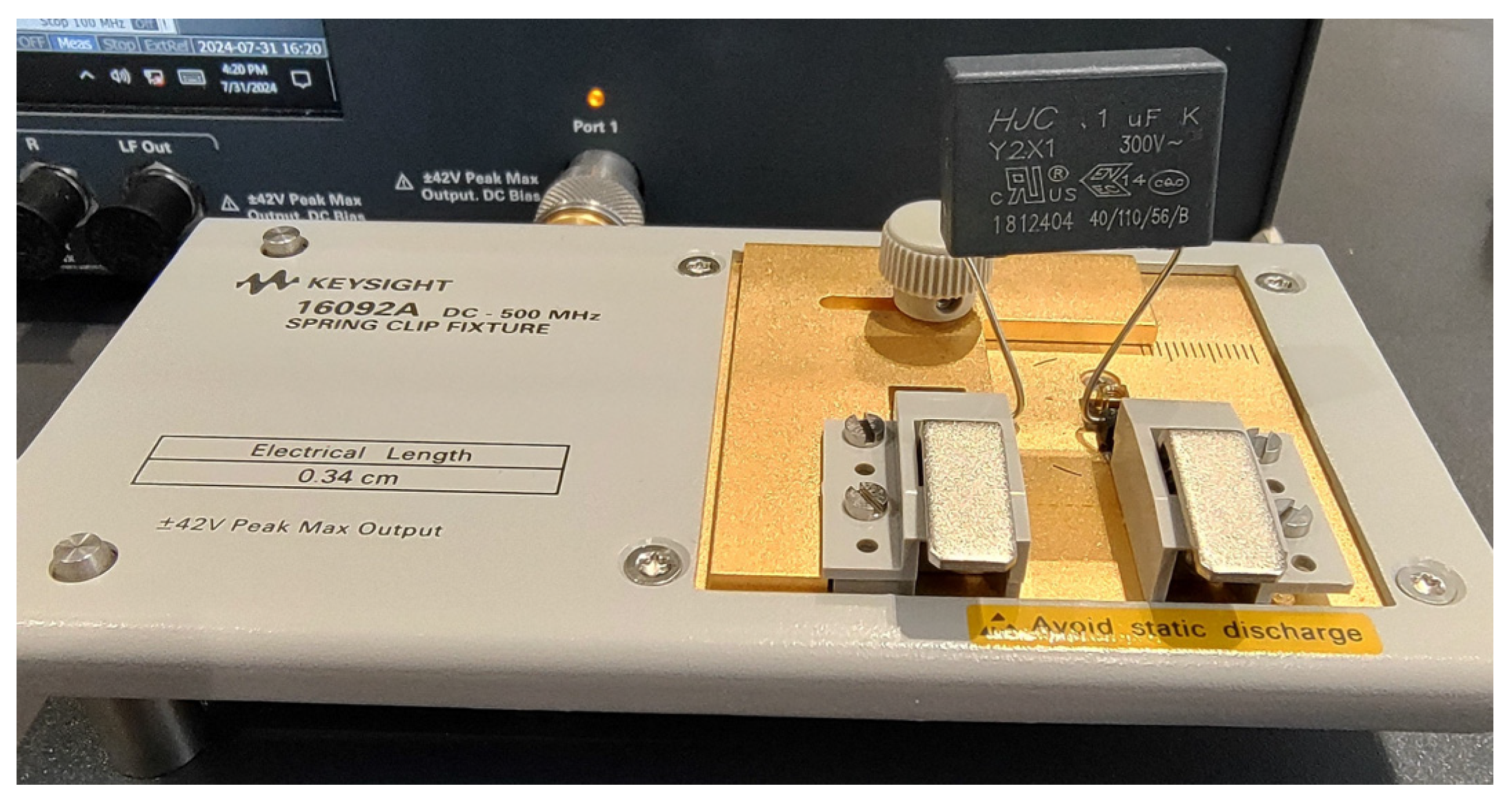
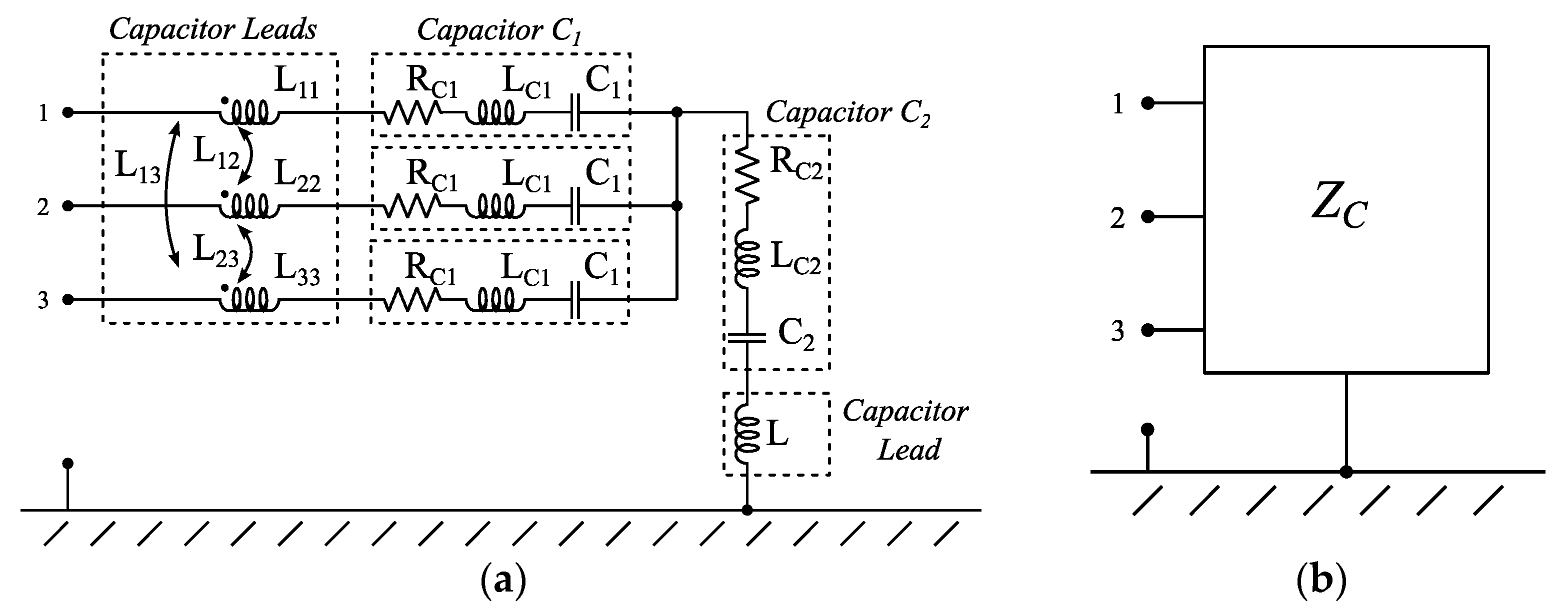
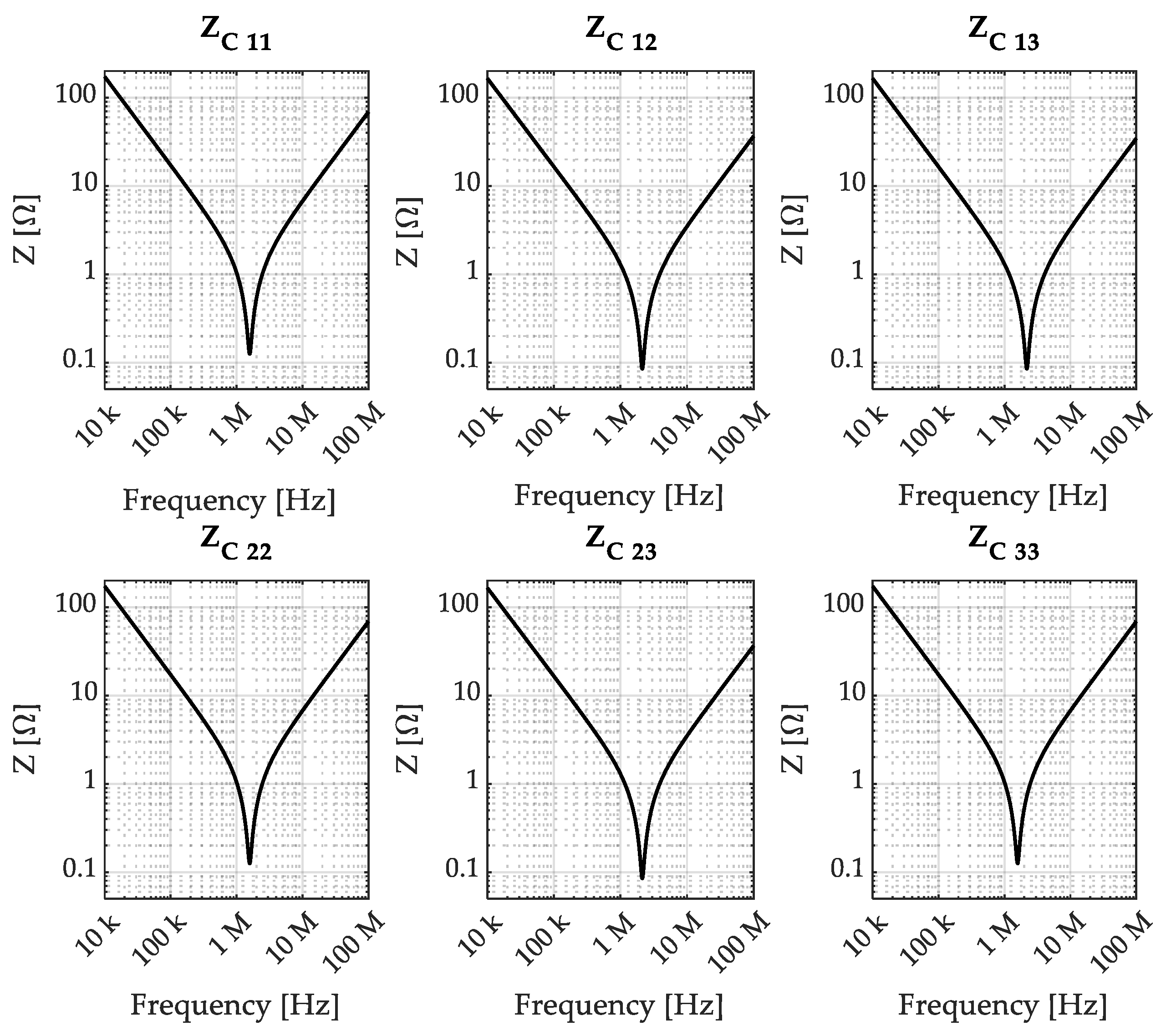
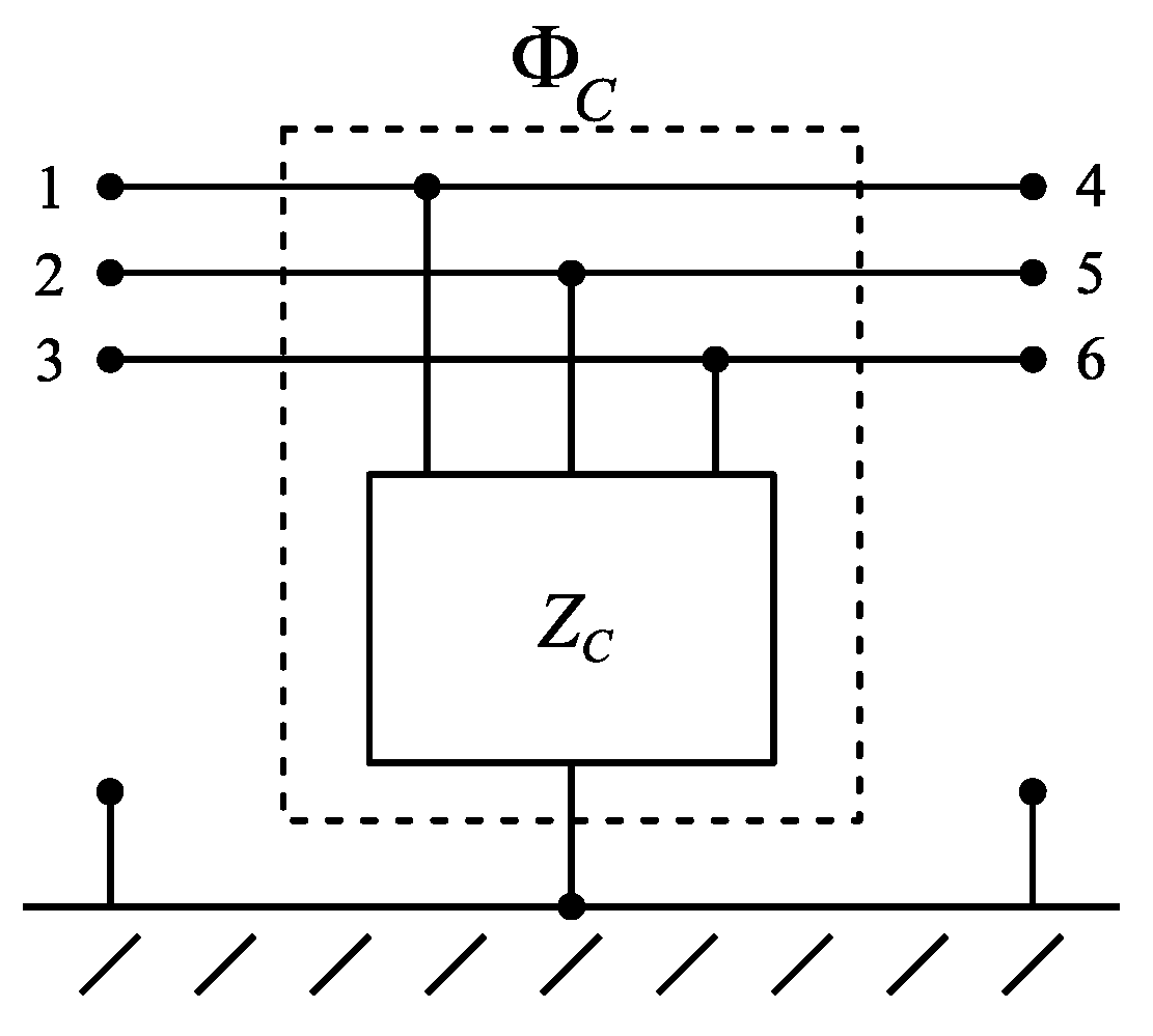
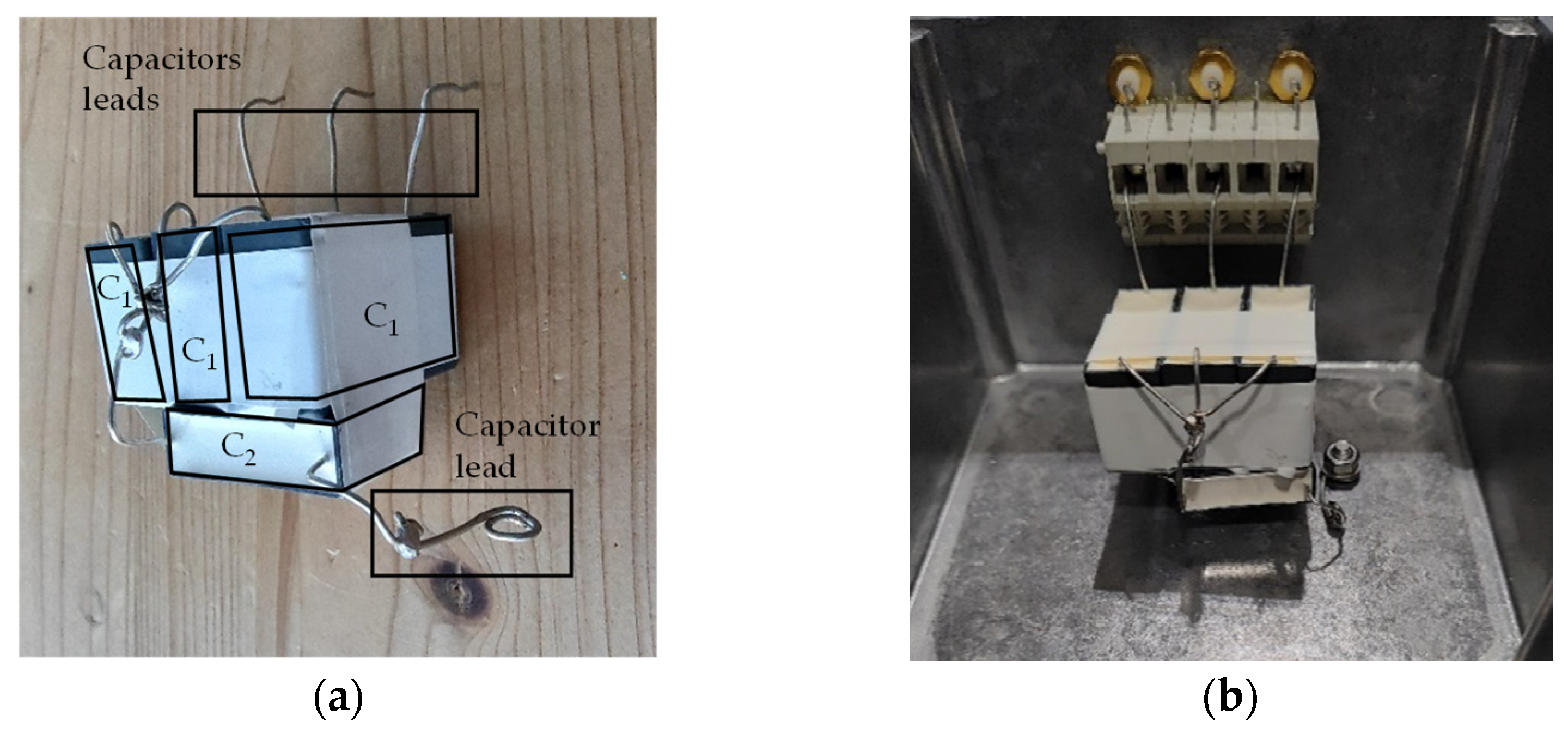
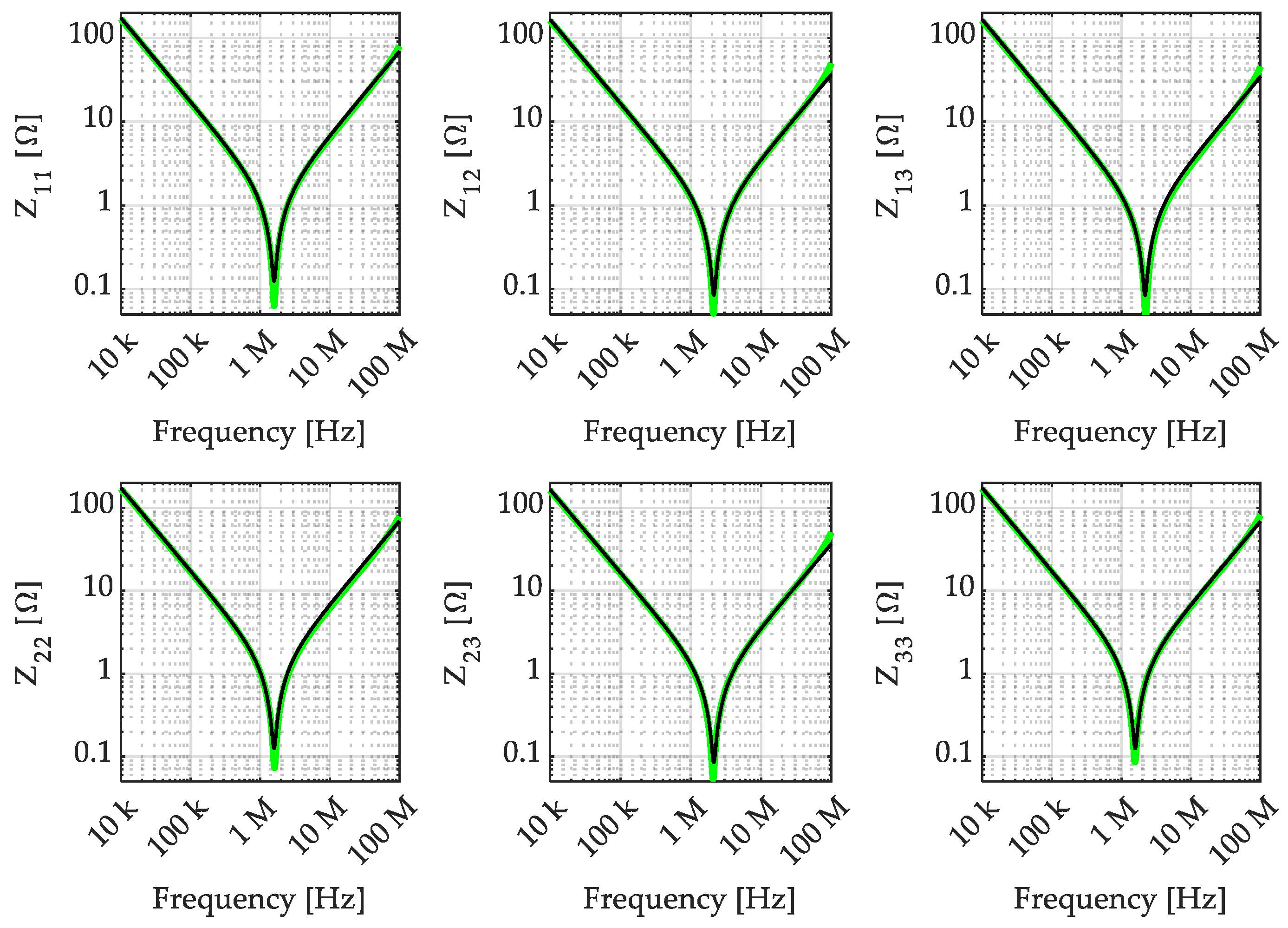
3.1. Capacitor Assembly Model

The first step for the characterization of the capacitor assembly is the characterization of at least one sample of each capacitor included in the assembly by an impedance analyzer (IA) or vector network analyzer (VNA) in order to determine the real frequency response of the specific components used. This, in turn, allows us to determine the real capacitance (C), equivalent series resistance (ESR), and equivalent series inductance (ESL) for each kind of capacitor used, obtained as average values over a broad frequency range. In particular, the value of C is obtained from the slope of the impedance frequency response up to a decade below the capacitor resonance frequency, the value of the ESL is obtained from the slope of the impedance frequency response from a decade higher than the resonance frequency, and the value of the ESR is obtained as an average value around the resonance frequency. Experience suggests that, for frequencies no higher than 100 MHz, this simple capacitor model is sufficient to obtain a reasonable level of accuracy. Nevertheless, the characterization procedure is necessary for each capacitor, as data provided in datasheets proved not to be reliable enough at frequencies higher than a few MHz.

With reference to the EMI filter depicted in Figure 1, one sample of each capacitor value has been tested by IA, as depicted in Figure 3. The resulting C, ESR, and ESL parameters are reported for each component, in

Table 1. Capacitors parameters.

	Rated C [nF]	Measured C [nF]	ESR [mΩ]	ESL [nH]
C1	2200	2208	40.42	33.89
C2	100	96.11	85.12	17.78

. This step is particularly relevant since the rated capacitance is not always representative of the real one due to standard production tolerances (e.g., C1 is very close to its rated capacitance, while C2 is roughly 4% smaller), and ESR and ESL values are difficult to estimate reliably without directly testing the capacitor.

While the ESR/ESL model is sufficient to approximate the frequency response of a single capacitor, it is not sufficient to accurately describe the overall capacitor assembly. It is well known from the literature that component leads introduce parasitic inductances, the effect of which is not negligible in the frequency range of interest. Indeed, considering the capacitor assembly included in the considered EMI filter, it is necessary to consider that its physical realization will be inside a metal box, close to one of its sides, and inclusive of non-negligible leads, with a length of several centimeters, and a distant of a few centimeters between each other and the metal box. In this situation, the lead realizing the connection to ground will exhibit a non-negligible inductance. Additionally, the three leads connecting the capacitor assembly to the filter external terminals will act as a three-phase mutual inductor. In both cases, the per-length inductances of the components leads are calculated by approximating the said leads as straight conductors floating above a ground plane, which significantly simplifies the mathematics of the problem with minimal impact on accuracy (note also that a more detailed model would require to measure a real sample). The resulting circuit model is reported in Figure 4. Formulas for the evaluation of per-length inductance parameters are available in [33].

With the aim of selecting a representation which can later be used to assess the model accuracy with respect to real measurements, it is convenient to represent the capacitor assembly by an impedance or admittance matrix, which can be easily characterized by three-port measurements. For reference, the entries of the impedance matrix Z_C obtained from the considered capacitor assembly model are reported in Figure 5, where, due to reciprocity, only the mutual terms above the main diagonal are reported.

Starting from its impedance matrix, the capacitor assembly can be easily represented as a six-port element, characterized by its chain-parameter matrix Φ_C, as depicted in Figure 6. The determination of the entries of the chain-parameter matrix Φ_C is straightforward, and results in

$${\Phi }_C=\left[\begin{array}{cc}{I}_3& 0_3\\ -{Z_C}^{-1}& I_3\end{array}\right],$$

(1)

where I₃ represents the 3 × 3 identity matrix, while 0₃ represents the 3 × 3 three zero matrix.

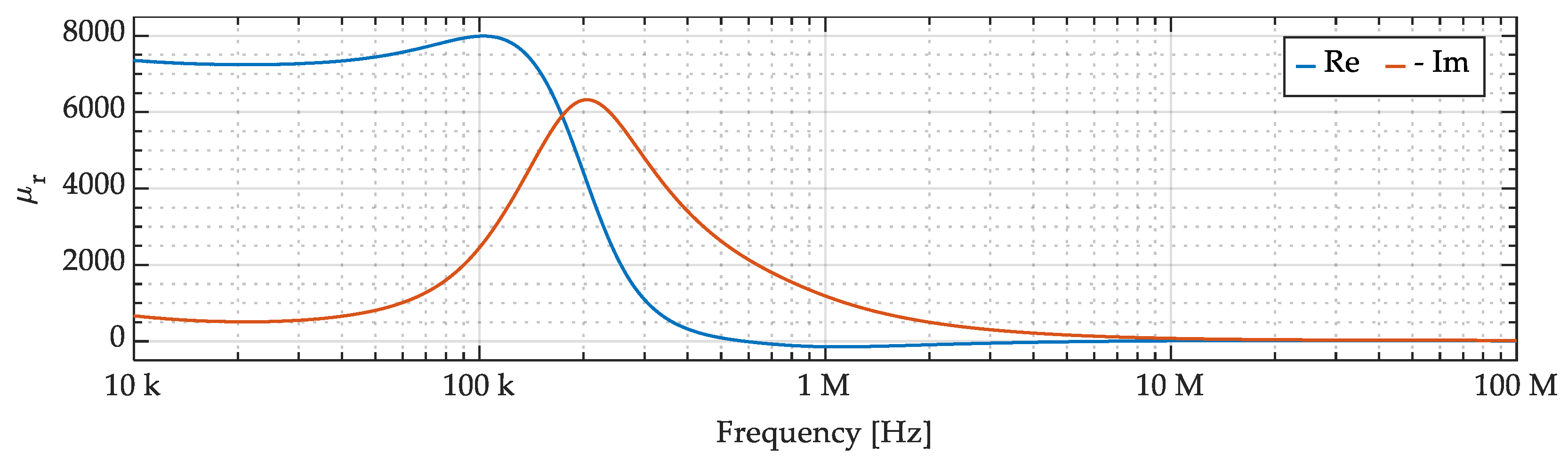
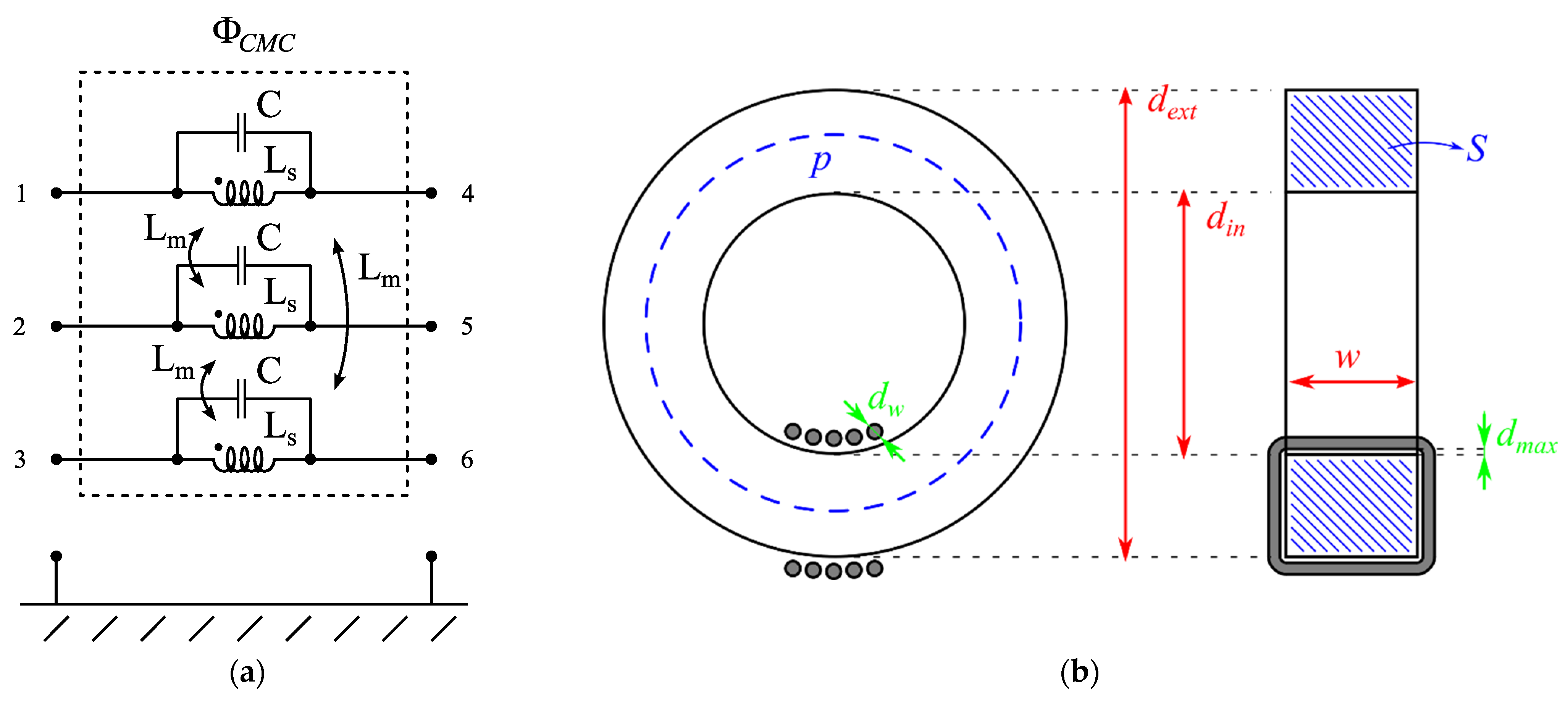
3.2. Common-Mode Choke and Interconnections Model

The first step for the definition of the CMC model is the characterization of the ferrite core complex permeability. This can be performed experimentally, which requires a non-trivial setup, or, alternatively, it is possible to rely on manufacturers’ data provided by datasheets. However, the suitability of the latter option for modeling purposes is questionable, as the characteristics of ferrite cores may be quite inconsistent among different samples, and manufacturers commonly declare a 20% to 30% tolerance on the magnetic permeability reported in datasheet. As a consequence, real measurements on a sample ferrite core are to be preferred whenever possible.

For reference, the measured magnetic permeability of the considered core, shown in Figure 2c, is reported in Figure 7.

It is worth noting that the complex behavior of the magnetic permeability over the frequency range of interest does not allow us to realize a simple circuit model (i.e., suitable to be included in SPICE simulations) of the CMC. As a consequence, unless complicated circuit synthesis techniques are employed, the physical model is limited to frequency-domain analysis and cannot be easily adapted to time-domain analysis. Indeed, while on the one side it is possible to determine an equivalent circuit representing the CMC frequency response accurately [34], this would basically be a behavioral model. In fact, most of the components appearing in the model would not have any physical meaning, but they would just fit the CMC frequency response. Also, it is not possible to determine the parameters of such a model without realizing a CMC prototype and characterizing it.

Once the complex, frequency-dependent magnetic permeability data regarding the selected core are available, a reasonably simple CMC model suitable for an industrial modeling procedure can be obtained considering:

• Core permeability and geometrical dimensions
• Number of turns of each winding (equal for each phase)
• Wire thickness, distance between wire turns and core, and distance between turns of the same winding

The considered CMC circuit model is reported in Figure 8a. It consists of a three-phase mutual inductor with parasitic capacitances, described by its self-inductance L_s, equal for all windings, its mutual inductances L_m, assumed equal for all winding pairs, and its parasitic capacitance C, also assumed equal for all windings. The CMC physical dimensions relevant to the evaluation of its parameters are highlighted in Figure 8b.

The expressions of the self-inductance L_s and of the mutual inductances L_m are obtained assuming the flux paths to develop completely in the ferrite core or in air, so that two inductances can be determined, namely:

$$L_{mag}=N^2{\mu }_0{\mu }_r{\displaystyle \frac{S}{p}}$$

(2)

$$L_{leak}=N^2{\mu }_0{\displaystyle \frac{\gamma \left(d_{ext}-d_{in}+2w\right)d_{\max }}{d_w\left(N-1\right)}}.$$

(3)

L_mag is defined as the inductance related to the flux path developed exclusively in the ferrite core, and is a function of the winding turn number N, the vacuum magnetic permeability μ₀, the ferrite core complex relative magnetic permeability μ_r, the core cross-section S, and the ferrite core mean perimeter p. The leakage inductance L_leak is defined as the inductance related to the flux in the air gap between the winding and the ferrite core.

It is a function of the winding turn number N, the vacuum magnetic permeability μ₀, the ferrite core geometric dimension d_ext (external diameter), d_in (internal diameter), and thickness w, the maximum distance between the winding and the ferrite core d_max, the winding wire thickness d_w, and the corrective coefficient γ. The latter is set, by empirical experience, between two and three for ferrite cores. All of these parameters are known or can be easily estimated even before realizing a single CMC prototype.

On the basis of the inductances L_mag and L_leak, the entries of the CMC inductance matrix are obtained assuming that the flux concatenating winding pairs is developed exclusively in the ferrite core, while the flux concatenating single windings develops both in the ferrite core and in air, separately. Consequently, the CMC self and mutual inductances are obtained as

$$L_s=L_{mag}+L_{leak},$$

(4)

$$L_m=L_{mag}.$$

(5)

The CMC inductance matrix is hence defined as

$$L_{CMC}=\left[\begin{array}{ccc}{L}_s& L_m& L_m\\ L_m& L_s& L_m\\ L_m& L_m& L_s\end{array}\right].$$

(6)

The parasitic capacitance is probably the least intuitive parameter to evaluate. Indeed, it would be intuitively stated that the parasitic capacitance value is proportional to the winding turn number. However, it has been proved that its value is mostly related to the geometrical dimensions of the single turns of a winding and is scarcely related to the total number of turns in the winding. Details on how to estimate this parameter are found in [35,36]. Considering the values of the geometrical parameters reported in

Table 2. Common-mode choke parameters.

Parameter	Value	Parameter	Value
Core Thickness	25.5 mm	Turns number	2
Core external diameter	63 mm	Wire-to-core distance	0.7 mm
Core internal diameter	37.5 mm	Wire thickness	1.6 mm
γ	2.5

(all readily available, except from the wire-to-core distance which is to be estimated), it is easy to determine the considered CMC inductance matrix L_CMC and parasitic capacitance C.

Hence, it is straightforward to evaluate the chain-parameter matrix Φ_CMC representing the CMC as

$${\Phi }_{CMC}=\left[\begin{array}{cc}{I}_3& -{\left(I_3-{\omega }^{2}C{L}_{CMC}\right)}^{-1}j\omega L_{CMC}\\ 0_3& I_3\end{array}\right].$$

(7)

This, however, can hardly be related with CMC measurements, as high-power CMCs are usually not mounted PCBs, but wound with single-core wires which extend to the filter terminals. Similar to capacitors assemblies leads, it is hence necessary to include wire interconnections in the CMC model.

Wire interconnections are approximated as three straight, bare, parallel wires with separation d, diameter d_w, running above ground at height h with length L. The chain-parameter matrix of such a multiconductor transmission line (MTL) section is easily computed [33]. For the CMC under consideration, two interconnections are to be considered. The parameters necessary to evaluate their chain-parameter matrices Φ_TL1 and Φ_TL2, estimated on the basis of the ferrite core and filter metal enclosure sizes, are reported in

Table 3. Cable interconnections parameters.

	Interconnection 1	Interconnection 2
Length	10 cm	5 cm
Separation	1.5 cm	1.5 cm
Wire diameter	1.6 mm	1.6 mm
Distance from ground	9 cm	9 cm

. The resulting CMC circuit model including wire interconnections modeled as MTLs is reported in Figure 9. Considering the cascaded connection of the two wire interconnections and the CMC, it is now possible to determine the CMC model by multiplying the relative chain-parameters matrices, namely,

$${\Phi }_{CMC+TL}={\Phi }_{TL2}{\Phi }_{CMC}{\Phi }_{TL1},$$

(8)

from which the CMC attenuation characteristics can be evaluated.

As the CMC CM and DM attenuations are usually its most relevant performance indexes, which can also be easily measured on real samples, the CM and DM attenuations obtained from the CMC model are evaluated. This is performed considering the circuits reported in Figure 10, which correspond to the CISPR-17 test setups for the measurement of the symmetrical (DM) and asymmetrical (CM) attenuation of an EMI filter.

Let us consider the standard testing condition, where R_S = R_L = 50 Ω, define the four minors of the CMC chain-parameters matrix as

$${\Phi }_{CMC+TL}=\left[\begin{array}{cc}{\Phi }_{CMC+TL\hspace{0.17em}\hspace{0.17em}11}& {\Phi }_{CMC+TL\hspace{0.17em}\hspace{0.17em}12}\\ {\Phi }_{CMC+TL\hspace{0.17em}\hspace{0.17em}21}& {\Phi }_{CMC+TL\hspace{0.17em}\hspace{0.17em}22}\end{array}\right],$$

(9)

and consider the DM attenuation between phases 1 and 2 A_{DM 12}, corresponding to the circuit reported in Figure 10a. The other two possible DM attenuations can be treated analogously.

By definition, the attenuation is obtained as

$$A_{DM\hspace{0.17em}12}={\displaystyle \frac{V_{DM\hspace{0.17em}12\hspace{0.17em}ref}}{V_{DM\hspace{0.17em}\hspace{0.17em}\hspace{0.17em}12\hspace{0.17em}}}},$$

(10)

where V_{DM 12} is the voltage across the load resistance R_L between terminals 1 and 2 obtained from the circuit in Figure 10a, and V_{DM 12 ref} is the same voltage obtained in the absence of the filter, which, under the condition R_S = R_L = 50 Ω, is equal to V_S/2. By tedious yet simple calculus, it is easy to prove that the voltages V₁, V_2, and V₃ in the circuit reported in Figure 10a can be obtained as

$$\left[\begin{array}{l}{V}_1\\ V_2\\ V_3\end{array}\right]=V_S{\left({\displaystyle \frac{1}{R_s}}{H}_1{\Phi }_{CMC+TL\hspace{0.17em}\hspace{0.17em}11}+{\displaystyle \frac{1}{{R_s}^2}}{H}_1{\Phi }_{CMC+TL\hspace{0.17em}\hspace{0.17em}12}{H}_1+{\Phi }_{CMC+TL\hspace{0.17em}\hspace{0.17em}21}+{\displaystyle \frac{1}{R_s}}{\Phi }_{CMC+TL\hspace{0.17em}\hspace{0.17em}22}{H}_1\right)}^{-1}{\displaystyle \frac{1}{R_s}}{K}_1,$$

(11)

where

$$H_1=\left[\begin{array}{ccc}-1& 1& 0\\ 1& -1& 0\\ 0& 0& 0\end{array}\right],\hspace{0.17em}\hspace{0.17em}{K}_1=\left[\begin{array}{c}-1\\ 1\\ 0\end{array}\right].$$

(12)

Once voltages V₁, V_2, and V₃ are known from (11), V_{DM 12} is obtained as

$$V_{DM 12}=V_1-V_2$$

(13)

and A_{DM 12} is easily evaluated from (10). The other DM attenuations A_{DM 23} and A_{DM 31} are similarly obtained from equations similar to (11)–(13), with the exception that H₁ and K₁ should be substituted with

$$H_2=\left[\begin{array}{ccc}0& 0& 0\\ 0& -1& 1\\ 0& 1& -1\end{array}\right],\hspace{0.17em}\hspace{0.17em}{K}_2=\left[\begin{array}{c}0\\ -1\\ 1\end{array}\right]$$

(14)

for the evaluation of A_{DM 23}, and with

$$H_3=\left[\begin{array}{ccc}-1& 0& 1\\ 0& 0& 0\\ 1& 0& -1\end{array}\right],\hspace{0.17em}\hspace{0.17em}{K}_3=\left[\begin{array}{c}1\\ 0\\ -1\end{array}\right]$$

(15)

for the evaluation of A_{DM 31}.

Consider now the CM attenuation A_CM, corresponding to the circuit reported in Figure 10b. By definition, the attenuation is obtained as

$$A_{CM\hspace{0.17em}}={\displaystyle \frac{V_{CM\hspace{0.17em}ref}}{V_{CM}}}$$

(16)

where V_CM is the voltage across the load resistance R_L, and V_{CM ref} is the same voltage obtained in the absence of the filter, which, under the condition R_S = R_L = 50 Ω, is equal to V_S/2. By tedious yet simple calculus, it is easy to prove that the voltage V_CM in the circuit reported in Figure 10b can be obtained as

$$V_{CM}=-R_S{1}_{1\times 3}\left[V_S{\left({R_S}^2{1}_3{\Phi }_{CMC+TL\hspace{0.17em}\hspace{0.17em}21}{1}_3-R_S{1}_3{\Phi }_{CMC+TL\hspace{0.17em}\hspace{0.17em}22}-R_S{\Phi }_{CMC+TL\hspace{0.17em}\hspace{0.17em}11}{1}_3+{\Phi }_{CMC+TL\hspace{0.17em}\hspace{0.17em}12}\right)}^{-1}\right]1_{3\times 1},$$

(17)

where 1_N×M denotes a N × M all-ones matrix. The resulting CMC CM and DM attenuation is reported, in magnitude and angle, in Figure 11.

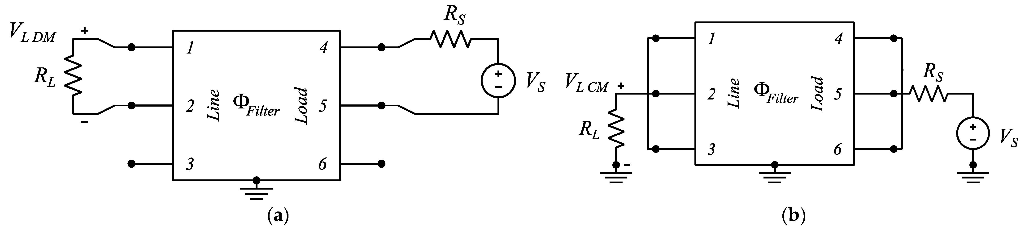
3.3. Complete EMI Filter Model

Once capacitor assemblies, CMC, and interconnection models are available in terms of chain-parameters matrices, and considering the components connections depicted in Figure 1, the overall EMI filter model can be obtained by simply cascading the corresponding chain-parameters matrices, namely,

$${\Phi }_{Filter}={\Phi }_{TL2}{\Phi }_{CMC}{\Phi }_{TL1}{\Phi }_C.$$

(18)

A flowchart summarizing the proposed EMI filter physical modeling procedure is reported in Figure 12.

Similar to the CMC, the CM and DM attenuation obtained from the considered physical EMI filter model is evaluated and reported, in magnitude and angle, in Figure 13.

3.4. Experimental Verification

In order to verify the accuracy of the considered modeling procedure and to discuss its limitations, the filter shown in Figure 1 was constructed, and its components were characterized separately at first, and then as a whole. Firstly, the capacitor assembly depicted in Figure 1 was realized, as shown in Figure 14a, where the correspondence between circuit elements and real components is highlighted. Successively, the capacitor assembly has been characterized as a three-port device by means of the setup depicted in Figure 14b.

To highlight how the considered simple model can effectively represent capacitor assemblies up to 100 MHz, the comparison between the impedance matrix entries obtained from the considered model, shown in Figure 5, and the measured impedance matrix entries are reported in Figure 15, from which it can be appreciated that the model accuracy is excellent over the whole frequency range of interest.

Secondly, the CMC shown in Figure 1 was constructed, as shown in Figure 16, where the correspondence between circuit elements and real components is highlighted. The comparison between the CM and DM attenuation obtained from the CMC model, shown in Figure 11, and their counterpart obtained from measurements of the CMC prototype shown in Figure 16 are reported, in magnitude and angle, in Figure 17.

It is possible to appreciate that the accuracy of the CM attenuation prediction, which is usually the most relevant CMC performance index, is excellent up to 1 MHz, while at higher frequencies the accuracy is progressively reduced. The accuracy of the DM attenuation prediction is excellent up to 1 MHz, while, similar to the CM attenuation, it is progressively reduced between 1 MHz and 100 MHz.

Such performance degradation can be ascribed to two reasons: Firstly, the decrease in the accuracy of the CM attenuation prediction can be related to the reduced ferrite core permeability. Indeed, comparing the attenuation in Figure 17 with the relative magnetic permeability in Figure 7, it is possible to appreciate that the frequency region where the model accuracy is poor (i.e., from 10 MHz to 100 MHz) corresponds to a frequency region where the magnetic material permeability is significantly reduced. As a consequence, the hypotheses introduced on flux paths, based on the ferrite core magnetic permeability being much larger than vacuum magnetic permeability, are no longer verified. Secondly, considering DM attenuation predictions, the discrepancies appearing in Figure 17 are mainly ascribed to constructive asymmetries in the real CMC shown in Figure 16, not included in the model.

Lastly, the complete EMI filter shown in Figure 1 was assembled as shown in Figure 18. The overall model accuracy is evaluated in terms of CM and DM attenuation, which is calculated from the considered model, as shown in Figure 13, and compared with measurements of the EMI filter prototype in Figure 19.

It can be observed that the filter CM attenuation prediction exhibits good accuracy up to 20 MHz, where the CMC model also exhibits good performance, and not very good accuracy between 20 MHz and 100 MHz, where the CMC model performance was poor. The filter DM attenuation prediction, on the other hand, exhibits quite a different behavior, as it is characterized by a small and almost constant magnitude error from around 500 kHz up to 80 MHz. Overall, the complete EMI filter model exhibits some limitations in terms of accuracy, as it can be expected on the basis of the limited accuracy of the CMC model. Nevertheless, it can be acceptable for virtual prototyping in industrial environments, as the considered physical model is quite easy and fast to use and allows the estimation of the performance of many different filter designs without the need for any prototypes.

4. Behavioral Modeling Procedure for Three-Phase EMI Filters

The behavioral modeling approach is based on external measurements only, which are usually S-parameters matrices measured by a VNA [16]. The literature about behavioral modeling techniques is indeed quite rich, and a comprehensive review lies outside the purposes of this paper. With no loss of generality, we will consider a recently proposed behavioral modeling technique [25], based on S-parameters characterization at the external ports [26], originally developed for single-phase EMI filters and here extended to three-phase filters. The considerations reported in the following apply to any other similar behavioral modeling techniques.

In the following, we will briefly recall the concepts of the considered behavioral modeling technique, and successively apply it to the three-phase EMI filter prototype presented in Figure 18.

4.1. EMI Filter Characterization and Rational Approximation of Its Frequency Response

The EMI filter under analysis is characterized as a multiport network, the frequency response of which is measured by a VNA [26]. On the basis of the measured EMI filter frequency responses, a rational approximation of its S-parameter matrix S is obtained by means of the VF algorithm [29,37], a well-known, robust iterative routine characterized by high computational efficiency and accuracy. The VF algorithm is also easily modified to include passivity enforcement techniques [30,31], necessary to obtain models suitable for time-domain simulations. The VF and its derivations are the results of a vast research activity in macro-modeling techniques, a comprehensive summary of which can be found in [38]. By applying the procedure discussed in detail in [25], the desired rational approximation is obtained as

$$S(s)={\displaystyle \sum _{k=1}^n\frac{1}{s-p_k}}{R}_k+D+sE$$

(19)

where s = jw is the complex frequency, p_k with k = 1,…, n is the set of n common poles, R_k is the residue matrix associated to each pole, and D and E are matrices which enforce the correct low-frequency asymptotic behavior.

4.2. Equivalent Circuit Synthesis

While the filter S-parameter matrix passive rational approximation (19) accurately represents the considered EMI filter, it is not suitable to be included in circuit solvers such as SPICE solvers. This limits its use in frequency-domain simulations and makes it impossible to run time-domain simulations. To overcome these limitations, a number of options are traditionally available, which are summarized in [38].

A more numerically efficient approach was proposed in [25], which is based on a concept originally explored in [39], and successively extended in [32]. It relies on the use of the poles and residues of the fitted S-parameter matrix to determine a circuit representation based on a fictitious branch admittance matrix Y_SB, having the same poles and residues of the fitted S-parameter matrix S. Once the frequency response of each branch is obtained, an equivalent circuit can be readily synthesized by resistors, inductors, and capacitors and translated into a SPICE netlist [40]. As discussed in [32,39], the fictitious branch admittance matrix Y_SB must be connected to the filter external ports by suitable controlled voltage sources. The extension of this concept to three-phase devices is shown in Figure 20. The set of controlled voltage sources in Figure 20 ensures that voltages and currents at the ports of the matrix Y_SB are numerically equal to the incident and reflect power waves, hence granting that the circuit reported in Figure 20 is a correct equivalent circuit. The set of controlled voltage and current sources can also be easily included in a SPICE netlist.

4.3. Experimental Verification

The overall equivalent circuit can then be included in a frequency-domain SPICE simulation (performed by LT SPICE [41]) realizing the setup presented in the CISPR 17 standard [14], as depicted in Figure 21, and the filter model attenuation can be evaluated. Of course, while a frequency-domain simulation of the considered equivalent circuit is the most efficient way to assess the model accuracy, the real model value lies in its suitability to both time- and frequency-domain simulations, as discussed in [24,25].

The CM and DM attenuation obtained from the aforementioned SPICE simulation is reported in Figure 22, where it is compared with the real EMI filter measured attenuation. It is possible to appreciate that the model accuracy is excellent over the whole frequency range of interest, with predicted and measured curves being almost perfectly superimposed.

5. Comparison of Physical and Behavioral Approaches for Virtual Prototyping and Accurate Modeling of Three-Phase EMI Filters

The physical model presented in Section 3 is based on the knowledge of capacitors frequency responses, CMC ferrite core magnetic permeability, and on an estimation of the filter enclosure size and of the used wire gauges. Capacitors frequency response and CMC ferrite core magnetic permeability can be measured or obtained from components datasheets, even though the latter option seems scarcely reliable. The considered model showed an overall acceptable accuracy for EMI filter virtual prototyping, as shown in Figure 19. Nevertheless, the model exhibits a significant error in CM attenuation magnitude between 20 MHz and 100 MHz, and a small yet no negligible error in DM attenuation magnitude from 500 kHz to 80 MHz. The real EMI filter imbalance is not appreciated in the model too, as the CMC model is symmetric by construction. While the CMC model can in principle be formulated including possible asymmetries, this would require a level of detail in its geometric parameters which would be hard to estimate without a reference protype.

By the analysis presented for capacitors assemblies and CMC models, it is possible to appreciate that the physical model of capacitor assemblies provides excellent accuracy, as shown in Figure 15, while the CMC model accuracy is limited over 10 MHz, as shown in Figure 17. This can be ascribed to the hypothesis introduced in Section 3.2 for CMC modeling, namely the flux path related to mutual inductances developing exclusively in the ferromagnetic core. This is a reasonable approximation as long as the ferromagnetic material relative magnetic permeability is large, yet, with reference to Figure 7, it can be appreciated that the magnetic permeability over 10 MHz is indeed quite small. As a consequence, at over 10 MHz the CMC fluxes are not confined by the ferromagnetic core, which implies that the windings coupling is related to air flux paths. This is not foreseen in the presented CMC model, as the modeling of such occurrence is quite difficult without a reference prototype. For modeling purposes, 3D electromagnetic simulations can be used to estimate the inductance in this condition, yet this option is not suitable for virtual prototyping, as the information needed for 3D simulation is usually not available in the absence of a real EMI filter prototype.

The considered physical model allows for a clear understanding of the relations between single components and overall filter performance, as it enables the comparison of many design variations with minimal effort and no need for any prototype. Additionally, it is suitable for frequency-domain simulation; yet, it is not the best option, in its current form, for time-domain simulations. This is due to the complex, frequency-depending ferrite magnetic permeability, which introduces complex, frequency-depending inductances to the model. These inductances cannot be integrated in a SPICE model as they are, and if time-domain simulations are required, it is necessary to determine a CMC equivalent circuit. However, this seems to be of limited interest, as time-domain simulations are usually used to assess the suitability of a specific filter for a given application, which is a task usually better addressed by behavioral models.

Considering the use of the considered physical model in an industrial context, its characteristics lend the model toward virtual prototyping. Due its limitations in accuracy and compatibility with time-domain simulations, it is not an optimal choice for a model to be distributed as additional material for commercial EMI filters to enable CE simulation by final users. Additionally, the distribution of such a model would require the disclosure of information on the filter internal structure, which is often considered proprietary information by EMI filter manufacturers.

The behavioral model presented in Section 4, on the contrary, is based on the external characterization of an EMI filter as a multiport electrical component. The considered model showed an excellent accuracy over the whole frequency range of interest, as shown in Figure 22. Being based on real measurements, the behavioral model can also correctly represent the real EMI filter imbalance; yet, relying on external measurements only, it does not allow any understanding of the relations between single components and overall filter performance. The present behavioral model is suitable for both time- and frequency-domain simulations, thanks to the specific formulation of the equivalent circuit presented in Section 4.2.

Considering the use of the presented physical model in an industrial context, its characteristics do not lend the model toward virtual prototyping, as it provides little help in understanding the complex relations between each component and the overall filter performance. On the other hand, the considered behavioral model allows the provision of a reliable and accurate filter representation to potential customers, without disclosing any information on the filter realization. As a consequence, it is an optimal choice for a model to be distributed as additional material for commercial EMI filter to enable CE simulation by the final user.

To conclude this section, a summary of the main aspects characterizing the considered physical and behavioral model is reported in

Table 4. Synthesis of the comparison between physical and behavioral EMI filter models.

	Physical Model	Behavioral Model
Required input	Capacitors frequency response and CMC ferrite cores magnetic permeability, estimated filter size	External measurement of the complete filter
Accuracy	Good up to 10 MHz, limited from 10 MHz to 100 MHz	Good over the whole frequency range of interest
Relation between single components and filter performance	Clear	Unclear
Suitable for virtual prototyping	Yes, allows fast comparison of many filter designs with no need for prototypes	No, requires one prototype to be built for each design of interest
Suitable for frequency-domain simulations	Yes	Yes
Suitable for time-domain simulations	Yes, but requires a behavioral CMC model to include the magnetic permeability frequency dependency in the model.	Yes
Suitable as a commercial model	No, requires to disclose details on the internal filter structure, limited accuracy	Yes, no proprietary information on filter realization is disclosed, high accuracy

.

6. Conclusions

This paper discussed and compared two common modeling approaches, namely, physical and behavioral, used for EMI filters. For both cases, an innovative procedure intended for application in the industrial context was discussed, considering a physical EMI filter modeling procedure first, which provides an overall filter model on the basis of minimal information on the filter components and does not require any prototype. The physical modeling approach is particularly suited for virtual prototyping, as it proved to be acceptably accurate with minimal information and no need for prototypes to test. The physical model was also verified step by step, highlighting the main underlying hypotheses introduced in its formulation and their impact on the overall model accuracy.

Successively, a behavioral EMI filter modeling procedure was presented, and its accuracy and applicability are discussed in detail. Lastly, an extensive comparison between the two EMI filter modeling approaches was presented. From the present analysis, the two considered modeling approaches appeared to be suitable for complementary use in industrial application, where physical modeling is best suited for the product developing and design phase, due its minimal computational effort and good accuracy, while the behavioral approach is best suited to verify which specific filter provides the best performance in a given application.

Future research will address improved physical modeling to reduce the discrepancies between measured and predicted CMC CM attenuation, and hence improve the overall filter model performance, hybrid models combining both physical and behavioral approaches, and non-linear effects in EMI filter attenuation.

References

1. Ran, L.; Gokani, S.; Clare, J.; Bradley, K.J.; Christopoulos, C. Conducted electromagnetic emissions in induction motor drive systems part I: Time domain analysis and identification of dominant modes. IEEE Trans. Electromagn. Compat. 1998, 13, 757–767. [Google Scholar]
2. Ran, L.; Gokani, S.; Clare, J.; Bradley, K.; Christopoulos, C. Correction to “Conducted Electromagnetic Emissions in Induction Motor Drive Systems Part II: Frequency Domain Models”. IEEE Trans. Power Electron. 1998, 13, 1229. [Google Scholar] [CrossRef]
3. Liu, Q.; Wang, F.; Boroyevich, D. Modular-Terminal-Behavioral (MTB) Model for Characterizing Switching Module Conducted EMI Generation in Converter Systems. IEEE Trans. Power Electron. 2006, 21, 1804–1814. [Google Scholar] [CrossRef]
4. Pérez, A.; Sánchez, A.-M.; Regué, J.-R.; Ribó, M.; Rodríguez-Cepeda, P.; Pajares, F.-J. Characterization of Power-Line Filters and Electronic Equipment for Prediction of Conducted Emissions. IEEE Trans. Electromagn. Compat. 2008, 50, 577–585. [Google Scholar] [CrossRef]
5. Laour, M.; Tahmi, R.; Vollaire, C. Modeling and Analysis of Conducted and Radiated Emissions Due to Common Mode Current of a Buck Converter. IEEE Trans. Electromagn. Compat. 2017, 59, 1260–1267. [Google Scholar] [CrossRef]
6. Liu, Y.; See, K.Y.; Yin, S.; Simanjorang, R.; Gupta, A.K.; Lai, J.-S. Equivalent circuit model of high power density SiC converter for common-mode conducted emission prediction and analysis. IEEE Electromagn. Compat. Mag. 2019, 8, 67–74. [Google Scholar] [CrossRef]
7. Rondon-Pinilla, E.; Morel, F.; Vollaire, C.; Schanen, J.-L. Modeling of a Buck Converter With a SiC JFET to Predict EMC Conducted Emissions. IEEE Trans. Power Electron. 2013, 29, 2246–2260. [Google Scholar] [CrossRef]
8. Rahman, M.A.; Sozer, Y.; De Abreu-Garcia, J.A. Reduction of Electromagnetic Interference (EMI) in Interleaved DC-DC Converters. In Proceedings of the 2020 IEEE Energy Conversion Congress and Exposition (ECCE), Detroit, MI, USA, 11–15 October 2020; pp. 3552–3557. [Google Scholar]
9. Harasis, S.K.; Haque, M.E.; Chowdhury, A.; Sozer, Y. SiC Based Interleaved VSI Fed Transverse Flux Machine Drive for High Efficiency, Low EMI Noise and High Power Density Applications. In Proceedings of the 2020 IEEE Energy Conversion Congress and Exposition (ECCE), Detroit, MI, USA, 30 October 2020; pp. 4943–4948. [Google Scholar]
10. Loschi, H.; Lezynski, P.; Smolenski, R.; Nascimento, D.; Sleszynski, W. FPGA-Based System for Electromagnetic Interference Evaluation in Random Modulated DC/DC Converters. Energies 2020, 13, 2389. [Google Scholar] [CrossRef]
11. Dey, S.; Mallik, A. A Comprehensive Review of EMI Filter Network Architectures: Synthesis, Optimization and Comparison. Electronics 2021, 10, 1919. [Google Scholar] [CrossRef]
12. Rebholz, H.M.; Tenbohlen, S.; Köhler, W. Time-Domain Characterization of RF Sources for the Design of Noise Suppression Filters. IEEE Trans. Electromagn. Compat. 2009, 51, 945–952. [Google Scholar] [CrossRef]
13. Bosi, M.; Sánchez, A.M.; Pajares, F.J.; Peretto, L. Three-Phase Modal Noise Analysis and Optimal Three-Phase Power Line Filter Design. Energies 2023, 16, 5461. [Google Scholar] [CrossRef]
14. CISPR 17, Methods of Measurement of the Suppression Characteristics of Passive EMC Filtering Devices; IEC: Geneva, Switzerland, 2011.
15. Dominguez-Palacios, C.; Gonzalez-Vizuete, P.; Martin-Prats, M.A.; Mendez, J.B. Smart Shielding Techniques for Common Mode Chokes in EMI Filters. IEEE Trans. Electromagn. Compat. 2019, 61, 1329–1336. [Google Scholar] [CrossRef]
16. Wang, S.; Lee, F.; Odendaal, W. Characterization and Parasitic Extraction of EMI Filters Using Scattering Parameters. IEEE Trans. Power Electron. 2005, 20, 502–510. [Google Scholar] [CrossRef]
17. He, R.; Xu, Y.; Walunj, S.; Yong, S.; Khilkevich, V.; Pommerenke, D.; Aichele, H.L.; Boettcher, M.; Hillenbrand, P.; Klaedtke, A. Modeling Strategy for EMI Filters. IEEE Trans. Electromagn. Compat. 2020, 62, 1572–1581. [Google Scholar] [CrossRef]
18. Kovacevic, I.F.; Friedli, T.; Musing, A.M.; Kolar, J.W. 3-D Electromagnetic Modeling of Parasitics and Mutual Coupling in EMI Filters. IEEE Trans. Power Electron. 2013, 29, 135–149. [Google Scholar] [CrossRef]
19. Kumar, M.; Jayaraman, K. Design of a Modified Single-Stage and Multistage EMI Filter to Attenuate Common-Mode and Differential-Mode Noises in SiC Inverter. IEEE J. Emerg. Sel. Top. Power Electron. 2021, 10, 4290–4302. [Google Scholar] [CrossRef]
20. Zhai, L.; Hu, G.; Lv, M.; Zhang, T.; Hou, R. Comparison of Two Design Methods of EMI Filter for High Voltage Power Supply in DC-DC Converter of Electric Vehicle. IEEE Access 2020, 8, 66564–66577. [Google Scholar] [CrossRef]
21. Mallik, A.; Ding, W.; Khaligh, A. A Comprehensive Design Approach to an EMI Filter for a 6-kW Three-Phase Boost Power Factor Correction Rectifier in Avionics Vehicular Systems. IEEE Trans. Veh. Technol. 2016, 66, 2942–2951. [Google Scholar] [CrossRef]
22. Zhai, L.; Yang, S.; Hu, G.; Lv, M. Optimal Design Method of High Voltage DC Power Supply EMI Filter Considering Source Impedance of Motor Controller for Electric Vehicle. IEEE Trans. Veh. Technol. 2023, 72, 367–381. [Google Scholar] [CrossRef]
23. Zhang, X.; Khodabandeh, M.; Amirabadi, M.; Lehman, B. A Simulation-Based Multifunctional Differential Mode and Common Mode Filter Design Method for Universal Converters. IEEE J. Emerg. Sel. Top. Power Electron. 2019, 8, 658–672. [Google Scholar] [CrossRef]
24. Negri, S.; Spadacini, G.; Grassi, F.; Pignari, S.A. Prediction of EMI Filter Attenuation in Power-Electronic Converters via Circuit Simulation. IEEE Trans. Electromagn. Compat. 2022, 64, 1086–1096. [Google Scholar] [CrossRef]
25. Negri, S.; Spadacini, G.; Grassi, F.; Pignari, S.A. Black-Box Modeling of EMI Filters for Frequency and Time-Domain Simulations. IEEE Trans. Electromagn. Compat. 2021, 64, 119–128. [Google Scholar] [CrossRef]
26. Haase, M.; Hoffmann, K.; Hudec, P. General Method for Characterization of Power-Line EMI/RFI Filters Based on S-Parameter Evaluation. IEEE Trans. Electromagn. Compat. 2016, 58, 1465–1474. [Google Scholar] [CrossRef]
27. Gustavsen, B.; Semlyen, A. Rational approximation of frequency domain responses by vector fitting. IEEE Trans. Power Deliv. 1999, 14, 1052–1061. [Google Scholar] [CrossRef]
28. Gustavsen, B. Improving the pole relocating properties of vector fitting. IEEE Trans. Power Deliv. 2006, 21, 1587–1592. [Google Scholar] [CrossRef]
29. Deschrijver, D.; Mrozowski, M.; Dhaene, T.; De Zutter, D. Macromodeling of multiport systems using a fast implemen-tation of the Vector Fitting method. IEEE Microw. Wireless Compon. Lett. 2008, 18, 383–385. [Google Scholar] [CrossRef]
30. Gustavsen, B.; Semlyen, A. Fast Passivity Assessment for $S$-Parameter Rational Models Via a Half-Size Test Matrix. IEEE Trans. Microw. Theory Tech. 2008, 56, 2701–2708. [Google Scholar] [CrossRef]
31. Gustavsen, B. Fast Passivity Enforcement for S-Parameter Models by Perturbation of Residue Matrix Eigenvalues. IEEE Trans. Adv. Packag. 2009, 33, 257–265. [Google Scholar] [CrossRef]
32. Negri, S.; Spadacini, G.; Grassi, F.; Pignari, S. Measurement-Based Equivalent Circuit Model for Time-Domain Simulation of EMI Filters. In Proceedings of the 2022 International Symposium on Electromagnetic Compatibility–EMC Europe, Gothenburg, Sweden, 5–8 September 2022; pp. 793–798. [Google Scholar]
33. Clayton, R.P. The TransmissionLine Equations for Multiconductor Lines. In Analysis of Multiconductor Transmission Lines; IEEE: Piscataway, NJ, USA, 2008; pp. 89–109. [Google Scholar]
34. Kotny, J.-L.; Margueron, X.; Idir, N. High-Frequency Model of the Coupled Inductors Used in EMI Filters. IEEE Trans. Power Electron. 2012, 27, 2805–2812. [Google Scholar] [CrossRef]
35. De Leo, A.; Cerri, G. A Charge Distribution Based Model for the Evaluation of an Air-Coil Stray Capacitance. IEEE Trans. Electromagn. Compat. 2019, 61, 1673–1677. [Google Scholar] [CrossRef]
36. Pasko, S.W.; Kazimierczuk, M.K.; Grzesik, B. Self-Capacitance of Coupled Toroidal Inductors for EMI Filters. IEEE Trans. Electromagn. Compat. 2015, 57, 216–223. [Google Scholar] [CrossRef]
37. Gustavsen, B. User’s Guide for Vectfit3. Available online: https://www.sintef.no/projectweb/vectorfitting/ (accessed on 17 July 2024).
38. Grivet-Talocia, S.; Gustavsen, B. Passive Macromodeling Theory and Applications; John Wiley & Sons: Hoboken, NJ, USA, 2016. [Google Scholar]
39. de Almeida, I.C. Frequency Domain Equivalent Circuit Modeling of Electromagnetic-Interference Filters through Scattering Parameters and Rational Approximation. Master’s Thesis, Department of Electronics, Information and Bioengineering, Politecnico di Milano, Milan, 2019. Available online: https://www.politesi.polimi.it/handle/10589/148940 (accessed on 17 July 2024).
40. Antonini, G. Spice equivalent circuits of frequency-domain responses. IEEE Trans. Electromagn. Compat. 2003, 45, 502–512. [Google Scholar] [CrossRef]
41. Linear Technology Inc. LTspice IV Getting Started Guide. 2011. Available online: https://www.analog.com/en/design-center/design-tools-and-calculators/ltspice-simulator.html (accessed on 17 July 2024).
Figure 1. Block scheme of the considered example of EMI filter.
Energies 17 04974 g001
Figure 2. (a) 2200 nF and (b) 100 nF capacitor samples, and (c) ferrite core sample used for the realization of the considered three-phase EMI filter prototype.
Energies 17 04974 g002
Figure 3. Capacitor characterization via IA.
Energies 17 04974 g003
Figure 4. Capacitor assembly circuit model (a) and its representation as impedance matrix (b).
Energies 17 04974 g004
Figure 5. Capacitor assembly impedance matrix entries prediction.
Energies 17 04974 g005
Figure 6. Capacitor assembly representation by chain-parameter matrix.
Energies 17 04974 g006
Figure 7. Ferromagnetic core complex magnetic permeability: real part (Re) and negative imaginary part (-Im).
Energies 17 04974 g007
Figure 8. Considered CMC circuit model (a) and relevant physical dimensions (b).
Energies 17 04974 g008
Figure 9. Considered common-mode choke circuit model, including wire interconnections modeled as multiconductor transmission lines.
Energies 17 04974 g009
Figure 10. CISPR-17 test setups equivalent circuit: (a) symmetrical (DM), and (b) asymmetrical (CM) attenuation.
Energies 17 04974 g010
Figure 11. CMC CM and DM attenuation prediction, in magnitude and angle.
Energies 17 04974 g011
Figure 12. Flowchart summarizing the proposed EMI filter physical modeling procedure.
Energies 17 04974 g012
Figure 13. Considered EMI filter CM and DM attenuation prediction, in magnitude and angle.
Energies 17 04974 g013
Figure 14. Capacitor assembly physical realization (a), and characterization setup (b).
Energies 17 04974 g014
Figure 15. Comparison between the capacitor assembly impedance matrix entries: model prediction (black) and measurement (green).
Energies 17 04974 g015
Figure 16. Considered common-mode choke prototype.
Energies 17 04974 g016
Figure 17. CMC CM and DM attenuation: comparison between model prediction and measurements, in magnitude and angle.
Energies 17 04974 g017
Figure 18. Considered EMI filter prototype.
Energies 17 04974 g018
Figure 19. Considered EMI filter CM and DM attenuation: comparison between physical model prediction and measurements, in magnitude and angle.
Energies 17 04974 g019
Figure 20. EMI filter SPICE-compatible equivalent circuit, directly obtained from the fitted scattering-parameter matrix S.
Energies 17 04974 g020
Figure 21. CISPR-17 test setups equivalent circuit: (a) symmetrical (DM), and (b) asymmetrical (CM) attenuation. The multiport element encloses the equivalent circuit explicitly represented in Figure 20.
Energies 17 04974 g021
Figure 22. Considered EMI filter CM and DM attenuation: comparison between behavioral model prediction and measurements, in magnitude and angle.
Energies 17 04974 g022