Abstract
Due to their nonlinear behavior and the harsh environments to which batteries are subjected, they require a robust battery monitoring system (BMS) that accurately estimates their state of charge (SOC) and state of health (SOH) to ensure each battery’s safe operation. In this study, the interacting multiple model (IMM) algorithm is implemented in conjunction with an estimation strategy to accurately estimate the SOH and SOC of batteries under cycling conditions. The IMM allows for an adaptive mechanism to account for the decaying battery capacity while the battery is in use. The proposed strategy utilizes the sliding innovation filter (SIF) to estimate the SOC while the IMM serves as a process to update the parameter values of the battery model as the battery ages. The performance of the proposed strategy was tested using the well-known B005 battery dataset available at NASA’s Prognostic Data Repository. This strategy partitions the experimental dataset to build a database of different SOH models of the battery, allowing the IMM to select the most accurate representation of the battery’s current conditions while in operation, thus determining the current SOH of the battery. Future work in the area of battery retirement is also considered.
1. Introduction
Owing to their high specific energy and high operational voltage, lithium-ion batteries (LiB) have received great attention and are used in many applications [1]. Unfortunately, LiB have a limited operational area mainly bound by two important parameters: voltage and temperature. As such, careful monitoring of a battery’s working temperature and voltage is necessary for its optimal and safe operation [2]. If the battery’s voltage exceeds its limit, the battery may develop dendrites over time, which increases the battery’s internal resistance, resulting in a lower output voltage. Moreover, if the working temperature is substantially increased, the battery may release toxic gases or burst into flames [3].
Another challenge presented by LiB technology is the accurate estimation of its available power or state of charge (SOC). SOC describes the amount of charge available in the battery at any given time during usage. SOC is often represented as a percentage value of available power vs. maximum power, or the available capacity vs. maximum capacity of the battery [3]. The main problem in determining the SOC is the absence of instrumentation that can accurately measure SOC during the battery’s operation. This results in an estimation problem where the SOC must be estimated using indirect measurements such as the battery’s terminal voltage and current [4].
Different techniques to estimate the LiB’s SOC have been proposed in the literature. Some techniques such as neural networks (NN) have been used with great success [5]; however, NN make use of extensive data that must be collected beforehand and are computationally expensive compared to other solutions [5]. Other techniques make use of electrochemical impedance spectroscopy (EIS) data, which requires special instrumentation to be installed in the system [6].
One popular SOC estimation solution is the ampere-hour counting method. The ampere-hour counting method determines SOC based on current measurements and the remaining capacity of the battery [3]. This method’s popularity relies on its simplistic approach. If the initial SOC is known, the previous SOC value can be subtracted or added based on the current profile. However, this method comes with many drawbacks. Its accuracy is highly dependent on the initial SOC value, correct current measurements, and accurate battery capacity readings [3]. To ensure proper estimates of the SOC, this method must be frequently calibrated; some calibration techniques include voltage-based corrections using lookup tables [3]. Another method was presented in [7], where the authors were able to jointly estimate the SOC and temperature at the same time. The ability to track the temperature in conjunction with the SOC provides useful insights in terms of battery life management and operational safety.
Furthermore, Kalman filters (KFs) present other estimation techniques that, when combined with the ampere-hour counting method, have proven to be accurate at estimating SOC. KFs provide an accurate and computationally inexpensive solution, but require an accurate battery model for their successful implementation [3]. A linear KF provides an optimal solution to the linear discrete estimation problem. However, due to the battery’s nonlinear nature, only modified versions of the KF have been used for SOC estimation. Some KF variations include the extended Kalman filter (EKF) and the unscented Kalman filter (UKF), among others [8,9]. Between these two strategies, the EKF is known to introduce instability in the estimation process due to the linearization process embedded in the algorithm [10]. On the other hand, the UKF has proven to be a more robust strategy [11,12]. Another robust strategy, known as robust fixed-lag smoothing, attempts to overcome model uncertainties or mismatch by utilizing the least favorable model over a finite time horizon [13]. This method is characterized by a dynamic game between two players: one player selects the least favorable model in a prescribed ambiguity set, while the other player selects the fixed-lag smoother, minimizing the smoothing error with respect to the least favorable model. Efficient implementation of the robust fixed-lag smoother may reduce computational burdens and avoid numerical instabilities, which may be helpful for battery applications.
Electrochemical and equivalent circuit models (ECMs) are among the most popular models for batteries. Electrochemical models are based on the underlying physics of the battery using 10–14 partial differential equations, resulting in highly complex and computationally demanding models, but providing high-accuracy information about the battery’s state. These types of models are often used for laboratory and battery development research [14,15,16,17].
On the other hand, ECMs represent the battery as an electric circuit using voltage sources, resistors, and capacitors. These types of models require low computational power and have low complexity, but are less accurate and yield little information about the battery [18]. Nevertheless, these traits allow for their implementation online.
Some ECMs studied include Rint model, Thevenin model, PNGV model, and Dual Polarity (DP) model [19]. These models can be differentiated by the number of Resistor–Capacitor (RC) branches in the circuit. Adding more RC branches allows the capture of higher-order nonlinearities, resulting in a more accurate model [19]. However, adding more RC branches increases the complexity and computational time of the algorithms.
In summary, a battery monitoring system (BMS) should be implemented to ensure safe operation of LiB. The BMS’s main function is the accurate estimation of the battery’s current SOC and operating temperature. In addition, the BMS can also track other parameters such as the battery’s state of health (SOH); SOH is a measurement of the current health of the battery and is sometimes calculated based on its available maximum capacity [20]. As the battery is subject to aggressive current profiles, excessive cycling, or regular use, its maximum battery capacity degrades over time [20]. Moreover, accurate estimation of the battery’s SOH can significantly increase the accuracy of the ampere-hour counting method, since it is dependent on the battery’s capacity [20]. Lastly, accurate tracking of the battery’s SOH allows for an effective planned retirement of the battery, which ensures that the system continues to operate optimally.
A battery is referred to as due for retirement once its SOH is at 80%, or in other words, when the battery’s maximum available capacity is at 80% or less of its designed capacity [20]. Battery retirement can be presented as a fault diagnosis problem, where a SOH value of 80% or lower signals a fault in the battery [21]. A recent paper presented a degradation empirical model-free battery end-of-life prediction framework [22]. This method utilized the KF and Gaussian process regression. It is important to note that the SOH should be rapidly tracked and updated for improved performance and reliability. The authors in [23] introduced a fast capacity estimation method as well as a fast accelerated degradation fault diagnosis strategy for SOH estimation. This article offers insights into the importance of tracking micro-health parameters in batteries, which directly correspond to the overall SOH of the battery or set of batteries.
The multiple model (MM) strategy has been used to detect faults in batteries [24]. In the MM strategy, several models representing different behaviors of the system are generated to make the algorithm resilient against uncertainty [25]. Moreover, [25] presented an interacting multiple model (IMM) strategy where the IMM was combined with the EKF to accurately estimate the SOC of a LiB. The IMM was given allowed two different variations of noise in the battery model to account for the different degrees of parameter shift during the estimation process. Lastly, in [26], a multiple model adaptive estimation (MMAE) technique was used for fault diagnosis. The proposed strategy made use of EIS data and EKFs to generate residual signals that were fed into an MMAE block to detect a fault in the battery.
This paper focuses on the implementation of a MM strategy, i.e., the IMM strategy, to estimate the battery’s capacity degradation while accurately estimating the SOC of a battery under cycling conditions [27]. This is a unique contribution to the field of battery monitoring, particularly when utilizing the relatively new sliding innovation filter (SIF). The experimental dataset was partitioned into sections representing a 100% SOH, 75% SOH, 50% SOH, 25% SOH, and 0% SOH, where each section can be identified as a mode to be used within the IMM algorithm. The motivation behind this partition is that the IMM would yield the best matching mode, thus identifying the current SOH of the battery.
The main contribution of this paper is the development of the SIF in conjunction with the IMM (the so-called SIF-IMM) for determining the SOC and SOH of a battery. The IMM algorithm is used for SOH estimation by partitioning the experimental dataset into several SOH modes. This strategy has not been presented in the literature. In addition to introducing this method, the paper compares the performances of SIF-IMM and KF-IMM in estimating SOH.
The remainder of the paper is structured as follows: Section 2 presents the battery and parameter models. Section 3 details the experimental data and estimation algorithms. Section 4 covers the artificial measurements. Section 5 describes the model parameter identification results. Section 6 presents the experimental setup and details the results of the proposed strategy. Section 7 presents the concluding arguments of the work.
2. Battery Models
This section presents the battery model used for the experiment.
Dual Polarity Model
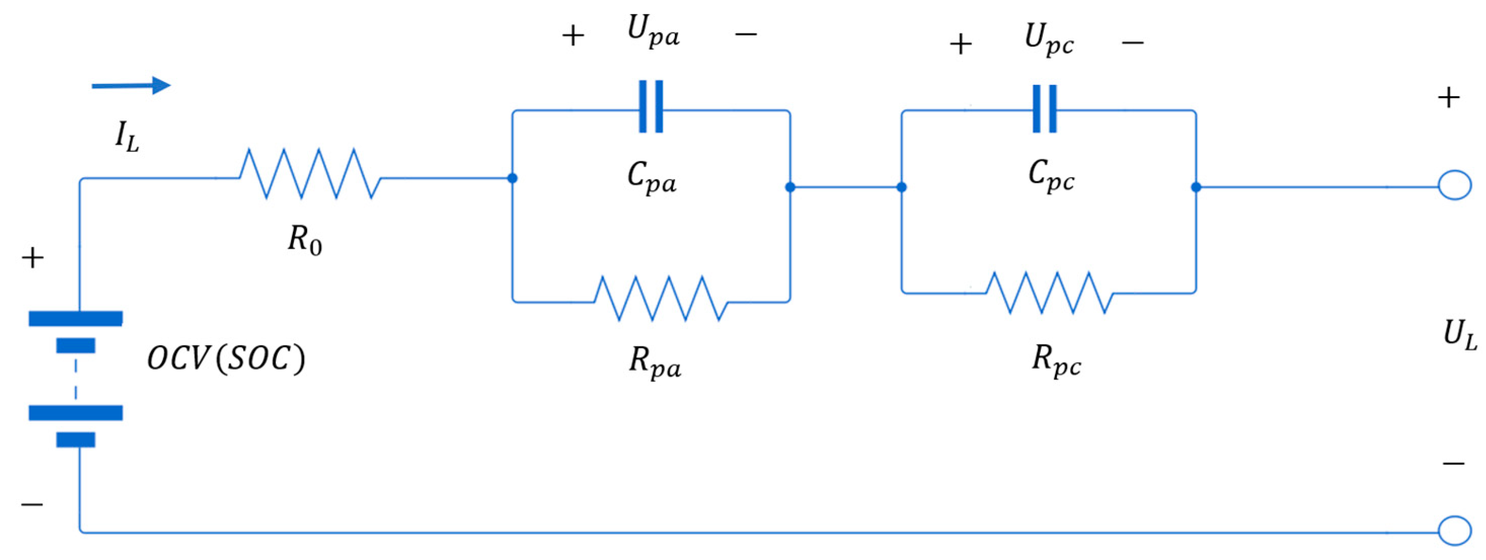
The DP model is an ECM composed of a voltage source, a resistor, and two RC-branches. These elements represent the battery’s output voltage, internal resistance, and short-term and long-term transient behaviors, respectively [16]. The battery’s transient behaviors are most noticeable at the end of a discharge charge, once the current is cut off. It is evident that there is a quick rise in voltage followed by a slower rise in voltage. These two phenomena have been attributed to the battery’s concentration polarization and electrochemical polarization, respectively. In the literature, the DP model has been shown to capture these behaviors by implementing a two RC-branch model [16]. The DP model was selected due to its high accuracy and ability to capture more nonlinearities while remaining computationally efficient. Figure 1 depicts the circuit diagram of the DP model.
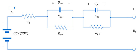
Figure 1.
DP model circuit architecture [16].
The circuit can be analyzed by breaking it down into three parts: , resistance, and capacitance. represents the open circuit voltage of the battery, represents the internal resistance of the battery, and and represent the electrochemical polarization resistance and concentration polarization resistance, respectively. Lastly, and characterize the transient response during the transfer of power to/from the battery during the electrochemical and concentration polarization [16].
Lastly, the system’s state space representation is described by the following equations:
3. Experimental Data and Estimation Algorithms
This section presents the selected experimental data and the estimation algorithms used for the experiments.
3.1. B005 DATASET
The B005 dataset is part of several datasets released by the Prognostic Center of Excellence (PCoE) and published by the Prognostic Data Repository for the advancement of prognostic algorithms [28]. This dataset provides cycling data of a 2 Ah battery up to a capacity of ~70%. The cycling data includes time, current, voltage, and temperature measurements for each cycle [28]. The B005 dataset was selected to test the proposed strategy as it provides data for each cycle. If the impedance data is counted, there are 615 cycles in total in this dataset. In this study, this dataset provides 340 discharge and charge cycles. The battery has an initial capacity of 1.856 Ah and is cycled to 1.303 Ah. Finally, the data was resampled from 3 s to 0.6 s to allow for improved algorithm adherence.
Figure 2 illustrates the battery capacity degradation over the 615 cycles.
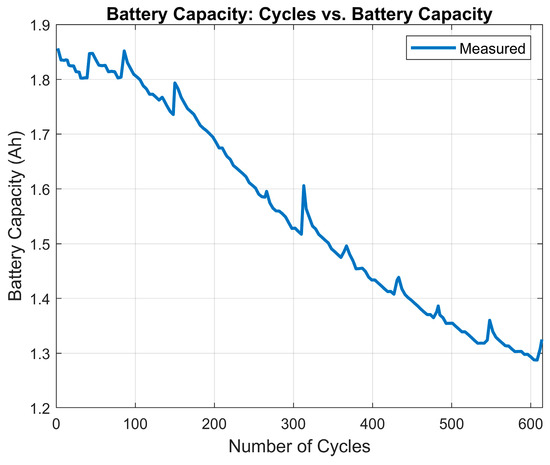
Figure 2.
Measured battery capacity at the end of each discharge cycle [29].
3.2. Ampere-Hour Counting
This method is the most popular for estimating SOC, where the SOC is estimated based on an initial value, i.e., , and this value is decreased/increased depending on the demanded/supplied current. SOC estimated using this method is given by [3]:
where is the initial SOC, is the nominal capacity of the battery, and is the discharge current.
3.3. Kalman Filter
The Kalman filter (KF) yields the optimal solution by minimizing the state estimation error for a known linear system that is subject to white Gaussian noise [30]. The linear system dynamics and the measurement model are described by the following two equations [31]:
where is the dynamics matrix, is the input matrix, is the output matrix, is the system states, is the measurement output, is the input, is the system noise, and is the measurement noise.
The KF algorithm is summarized in two stages: prediction and update [30].
- (i)
- Prediction Stage:
- (ii)
- Update Stage:where and are the system and measurement noise covariance matrices, respectively.
3.4. Sliding Innovation Filter
A recently proposed estimation strategy is the novel sliding innovation filter (SIF). The SIF was formulated based on a predictor–corrector estimation method [32]. Like the KF, the SIF first makes predictions of the state estimates and state error covariances using values from previous time steps, and then updates the predictions based on the measurements and a correction term referred to as the SIF gain [32].
The main difference between the SIF and KF algorithms is how the gain was constructed. The SIF gain was built using the measurement matrix, the innovation, and a sliding boundary layer term [32]. On the other hand, the KF makes use of the state error covariance. In other words, the SIF makes use of the gain to drive the state estimates within the defined boundary layer and forces the state estimates to switch about the true trajectory [32]. The following equations describe the SIF algorithm [32].
- (i)
- Update Stage:
Note that refers to the pseudoinverse of , refers to the diagonal of the saturation term (value between and ), and is the sliding boundary layer width.
3.5. Interacting Multiple Model (IMM)
The IMM method is most useful for systems with more than one operating mode. The IMM algorithm utilizes a number of models and computes the likelihood values for each model based on the state estimates and the corresponding state error covariance. The likelihood value is also based on the innovation (or measurement error) and provides an indication of how similar the actual system’s behavior is compared to the filter model. These likelihood values are then used to determine the operating mode [33]. Note that the IMM is essentially a set of filters that run in parallel, with each filter utilizing a different dynamic system and/or measurement model. The IMM algorithm can be described in a set of five stages. These five stages are presented below [33].
- (i)
- Calculation of the mixing probabilities :where refers to the mixing probabilities between modes and at time , refers to the mixing parameter (predefined value), and refers to the mode probability.
- (ii)
- Mixing Stage:where and are the state estimates and state error covariances used as initial conditions for the filters (KF or SIF).
- (iii)
- Mode-Matched Fitlering:where refers to the likelihood value generated based on the measurement, estimate measurement (from the corresponding filter), and the innovation covariance matrix (from the corresponding filter). The likelihood value is then used to update the mode probability (described in the next stage).
- (iv)
- Mode Probability Update:
- (v)
- State Estimate and Covariance Combination
Note that for this final stage (v), the overall state estimates and state error covariance are used outside of the IMM process, and are used for output purposes only.
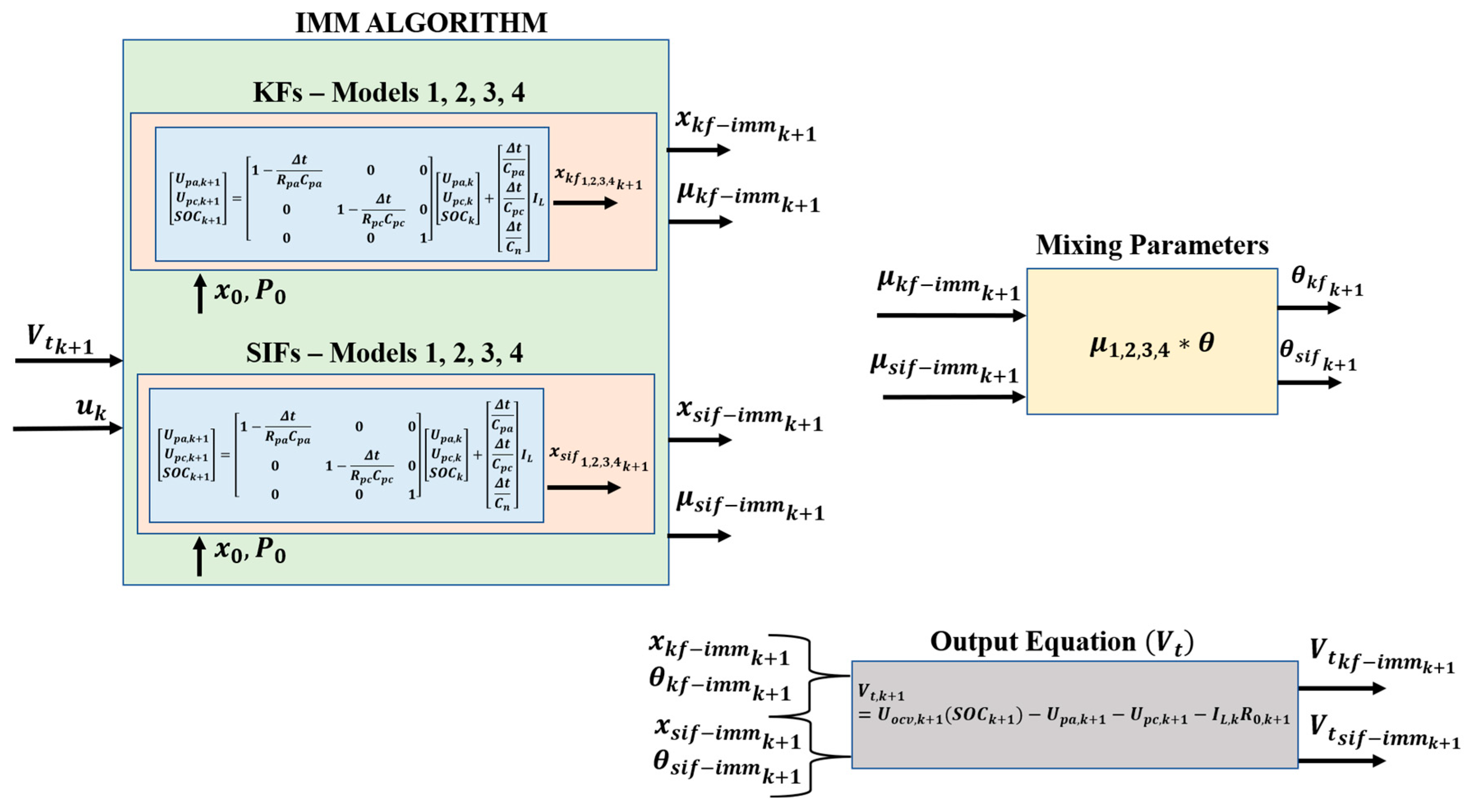
In the proposed strategy, the IMM is used to track the correct battery capacity, thus estimating the SOH of the battery. Meanwhile, the KF and SIF are used to estimate the SOC of the battery during cycling. The integration of these algorithms with the IMM resulted in strategies referred to as KF-IMM and SIF-IMM. The figure shown in Appendix A helps to further illustrate the overall architecture of the proposed strategies.
4. Artificial Measurements
As mentioned in Section 3.4, the SIF gain was derived based on the measurement matrix, meaning that it is dependent on the availability of individual measurements for each state estimate [32]. When individual measurements for each state are not available, which is often the case for LiBs and most types of batteries, generating artificial measurements is necessary to ensure that the SIF is effective [32]. The SIF strategy relies on the measurements in order to formulate good estimates of the states through the use of a full identity measurement matrix. This is one of the main disadvantages of this method. This section presents how artificial measurements were generated for the battery and parameter model.
4.1. State Measurement Equations
LiBs only offer measurements of current, voltage, and temperature. To generate artificial measurements for each state of the battery model, the model equations were rearranged as followed:
where , , and are the measurements for each state of the battery model, and is the inverse function of found in (27).
4.2. Parameter Measurement Equations
To generate artificial measurements for the parameters of interest, and , Equations (2) and (3) were rearranged as follows:
where and represent the artificial measurements for and .
5. Model Parameter Identification
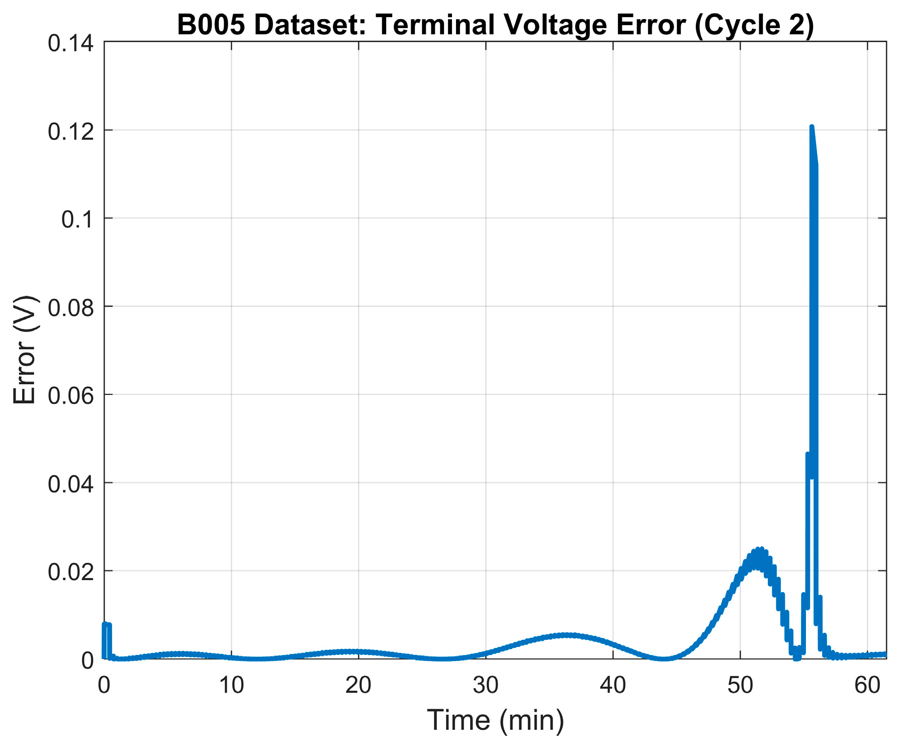
As mentioned before, the IMM makes use of several models. These models were identified by breaking the B005 dataset into four regions, resulting in five different modes to be identified corresponding to 100%, 75%, 50%, 25%, and 0% SOH. Furthermore, the B005 dataset contains 340 discharge and charge cycles; however, only the discharge cycles provide battery capacity measurements. Since this paper focuses on battery capacity estimation, the models were derived using discharge cycles. To derive each battery model, the following parameters needed to be identified (for each of the selected cycles): . This section presents the model’s parameter identification results using the nonlinear least squares (NLLS) algorithm for each of the modes selected: 100%, 75%, 50%, 25%, and 0% SOH.
5.1. Least Squares Setup
To use the NNLS algorithm, a relationship between the measurable data and the parameters must be established. Making use of the battery model, the following relationship can be derived [29]:
where represents the time vector, is the curve approximated to a 5th order polynomial, and represents the parameter vector, i.e., a vector consisting of all the parameters. Here, the capacitance values are estimated using a fraction to account for their higher magnitude [29,34].
Lastly, MATLAB®’s R2023a ‘’ function was used to perform the parameter estimation process. This function makes use of boundaries and initial conditions which are detailed in Table 1.

Table 1.
NLLS boundaries and initial guess.
5.2. Least Squares Results
5.2.1. The 100% SOH Model
As indicated before, 100% SOH represents a battery with an available capacity equal to its designed capacity. Table 2 shows the results of the parameter identification process for the 100% SOH mode. The terminal voltage’s RMSE was 0.063 V. Figure 3 depicts the terminal voltage’s error plot between the model and the measured terminal voltage. Finally, Figure 4 illustrates the generated model’s terminal voltage plot vs. the measured terminal voltage.

Table 2.
NLLS parameter estimation results for 100% SOH model.
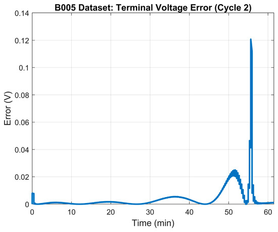
Figure 3.
100% SOH: LS model error—terminal voltage.
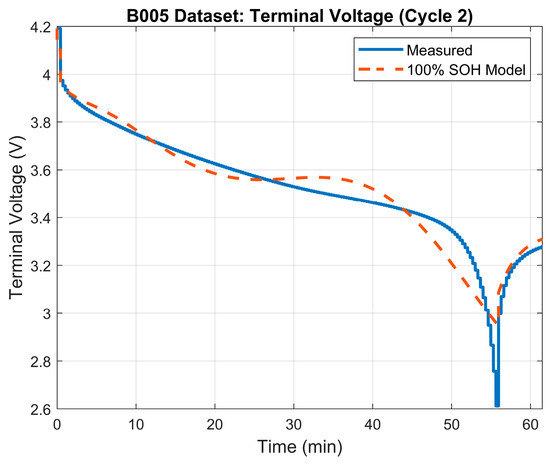
Figure 4.
Terminal voltage: model vs. measured voltage for 100% SOH model.
5.2.2. The 75% SOH Model
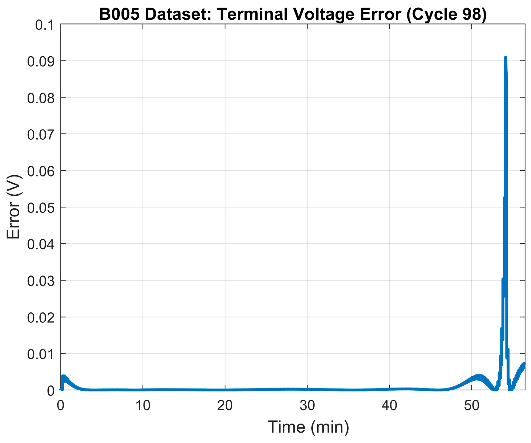
The 75% SOH of the battery was determined to occur when the battery reaches a capacity of 1.83 Ah which, based on the data, happens at the ~98th cycle. Table 3 illustrates the results of the parameter identification process for the 75% SOH mode. The terminal voltage’s RMSE was 0.032 V. Figure 5 depicts the terminal voltage’s error plot between the model and the measured terminal voltage. Figure 6 shows the generated model’s terminal voltage plot vs. the measured terminal voltage.

Table 3.
NLLS parameter estimation results for 75% SOH model.
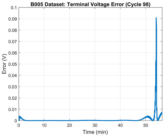
Figure 5.
75% SOH: LS model error—terminal voltage.
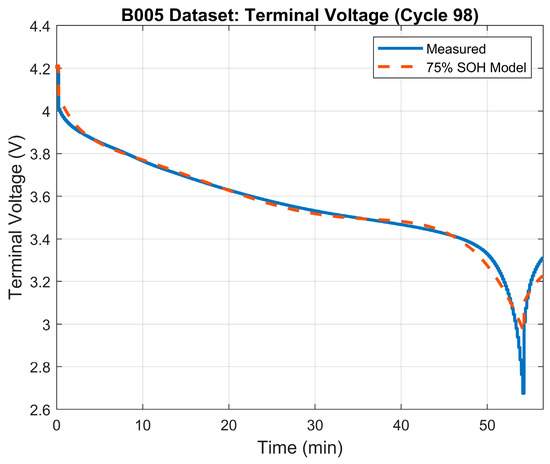
Figure 6.
Terminal voltage: model vs. measured voltage for 75% SOH model.
5.2.3. The 50% SOH Model
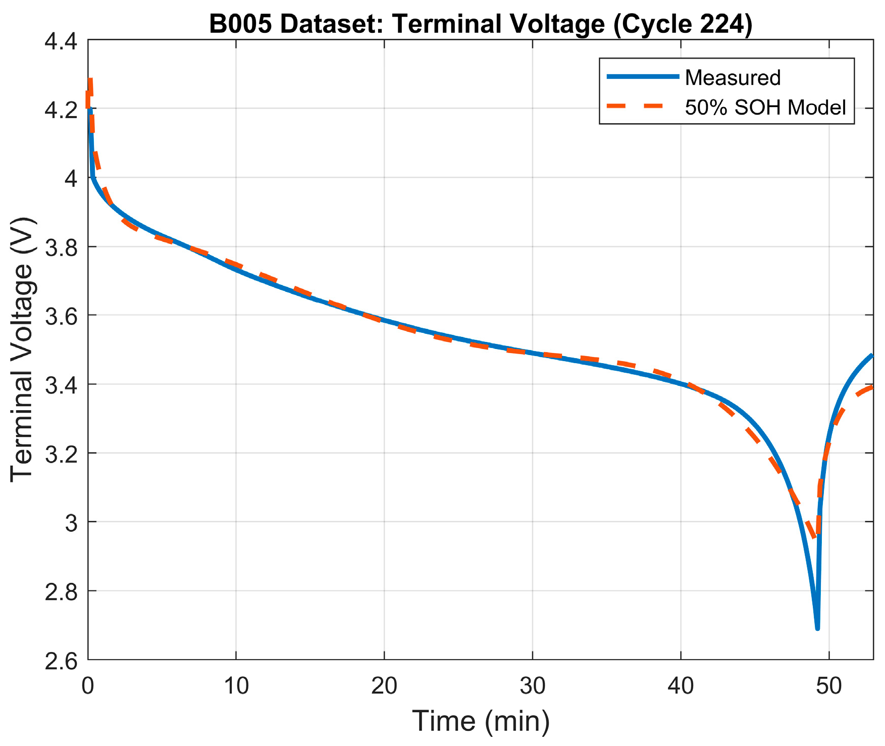
The 50% SOH of the battery was determined to occur when the battery reaches a capacity of 1.65 Ah which, based on the data, happens at the ~225th cycle. Table 4 illustrates the results of the parameter identification process for the 50% SOH mode. The terminal voltage’s RMSE was 0.032 V. Figure 7 shows the terminal voltage’s error plot between the model and the measured terminal voltage, and Figure 8 illustrates the generated model’s terminal voltage plot vs. the measured terminal voltage.

Table 4.
NLLS parameter estimation results for 50% SOH model.
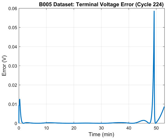
Figure 7.
50% SOH: LS model error—terminal voltage.
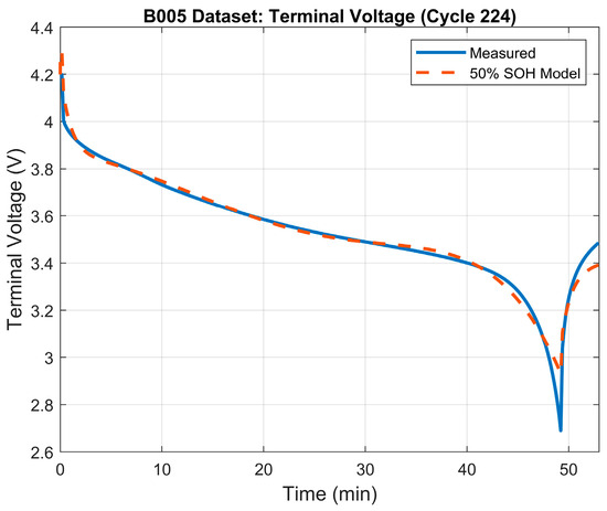
Figure 8.
Terminal voltage: model vs. measured voltage for 50% SOH model.
5.2.4. The 25% SOH Model
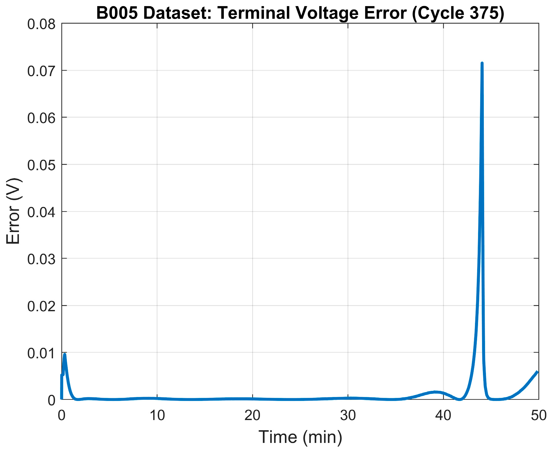
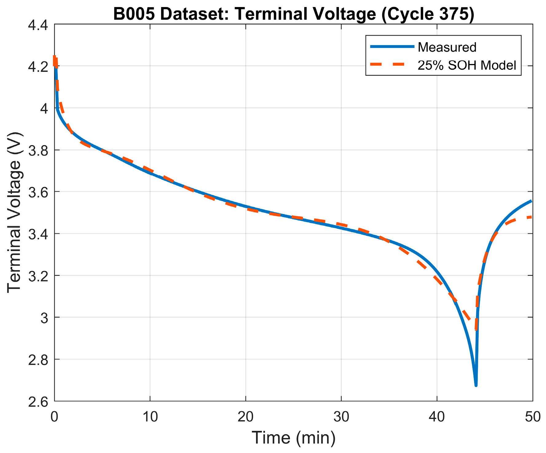
The 25% SOH of the battery was determined to occur when the battery reaches a capacity of 1.48 Ah which, based on the data, happens at the ~375th cycle. Table 5 illustrates the results of the parameter identification process for the 25% SOH mode. The terminal voltage’s RMSE was 0.034 V. The terminal voltage’s error plot between the model and the measured terminal voltage is depicted in Figure 9. The generated model’s terminal voltage plot vs. the measured terminal voltage in shown in Figure 10.

Table 5.
NLLS parameter estimation results for 25% SOH model.
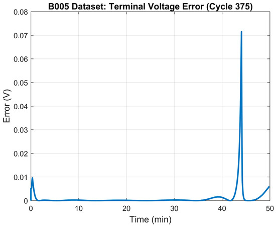
Figure 9.
25% SOH: LS model error—terminal voltage.
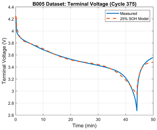
Figure 10.
Terminal voltage: model vs. measured voltage for 25% SOH model.
5.2.5. The 0% SOH Model
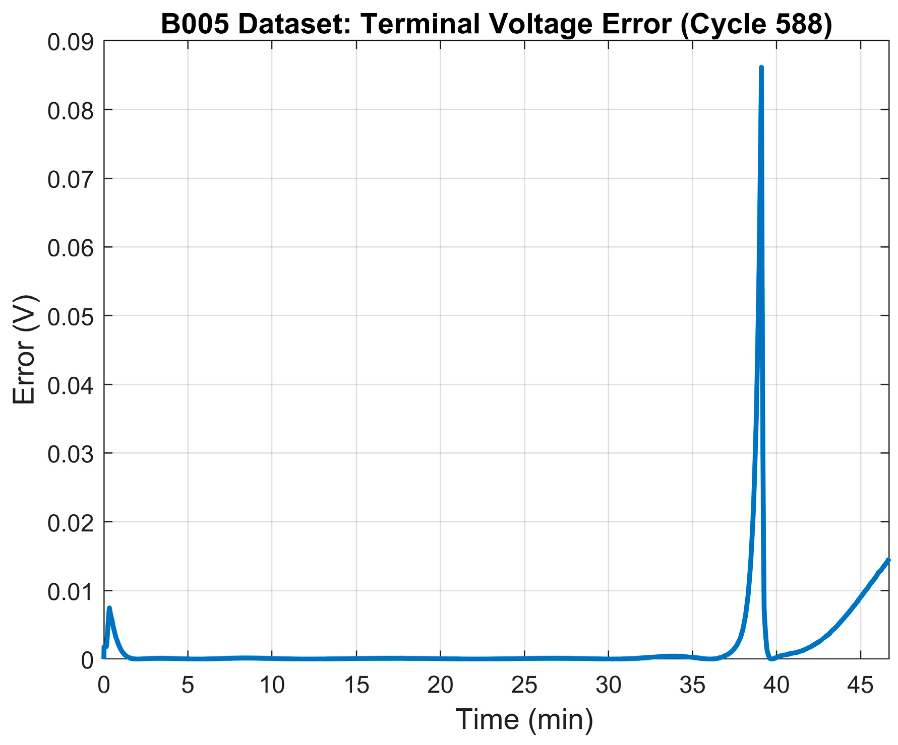
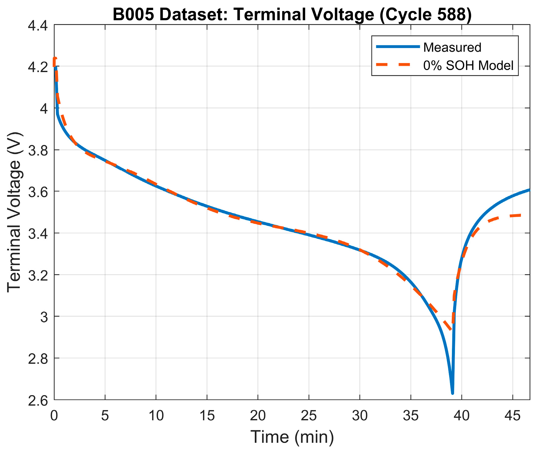
The 0% SOH of the battery occurs when the battery reaches a capacity of 1.30 Ah which, based on the data, happens at the ~588th cycle. Table 6 illustrates the results of the parameter identification process for the 0% SOH mode. The terminal voltage’s RMSE was 0.042 V. Figure 11 shows the terminal voltage’s error plot between the model and the measured terminal voltage. The generated model’s terminal voltage plot vs. the measured terminal voltage is illustrated in Figure 12.

Table 6.
NLLS parameter estimation results for 0% SOH model.

Figure 11.
0% SOH: LS model error—terminal voltage.
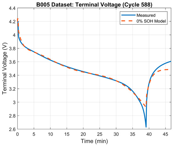
Figure 12.
Terminal voltage: model vs. measured voltage for 0% SOH model.
6. Simulation Setup and Results
6.1. Simulation Setup
Mode Matching
In this experiment, the IMM was used for tracking the battery capacity of the LiB. The IMM was combined with the KF and SIF, resulting in the KF-IMM and SIF-IMM algorithms. The initial mode probabilities were set to 95% normal and 5% faulty. The IMM mixing parameter was defined as . Initial estimates were set to zero.
The IMM has access to five different battery models representing different stages of the SOH of the battery. As the battery ages, the IMM selects the mode that best matches the battery’s current state and by doing so, the battery’s current SOH can be determined. Table 7 summarizes the initial conditions used for this experiment.

Table 7.
Mode matching experiment: initial conditions.
6.2. Simulation Results
This section presents the results obtained from the proposed strategy.
Mode Matching
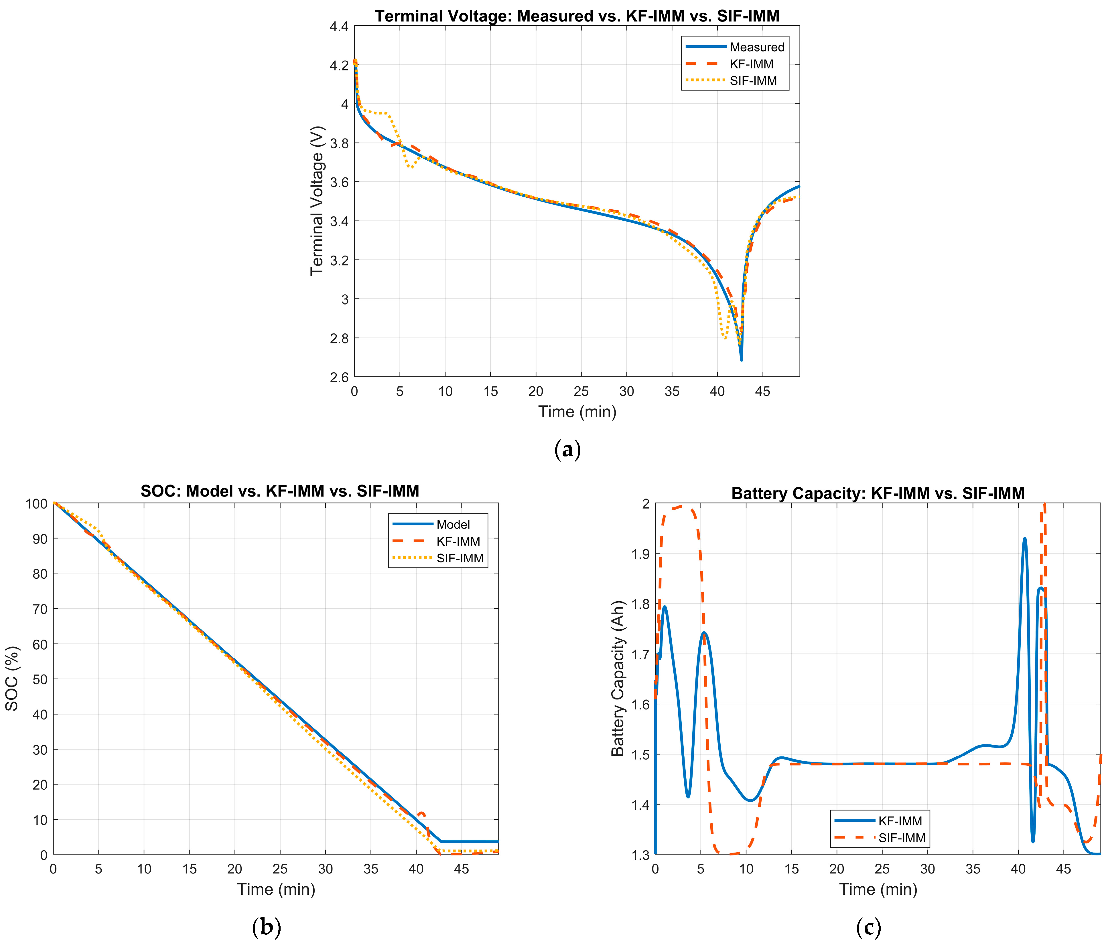
Five different modes were identified in the B005 dataset and served as the database for the IMM algorithm. At the end of each time step of each cycle, the parameter values of each mode were multiplied by the probability of each mode and combined to determine the estimated parameter values of the proposed IMM strategy. The following cycles were chosen to demonstrate the results of the proposed strategy at each stage of SOH: 106, 278, 441, 596. These cycles correspond to 75% SOH, 50% SOH, 25% SOH, and 0% SOH, respectively.
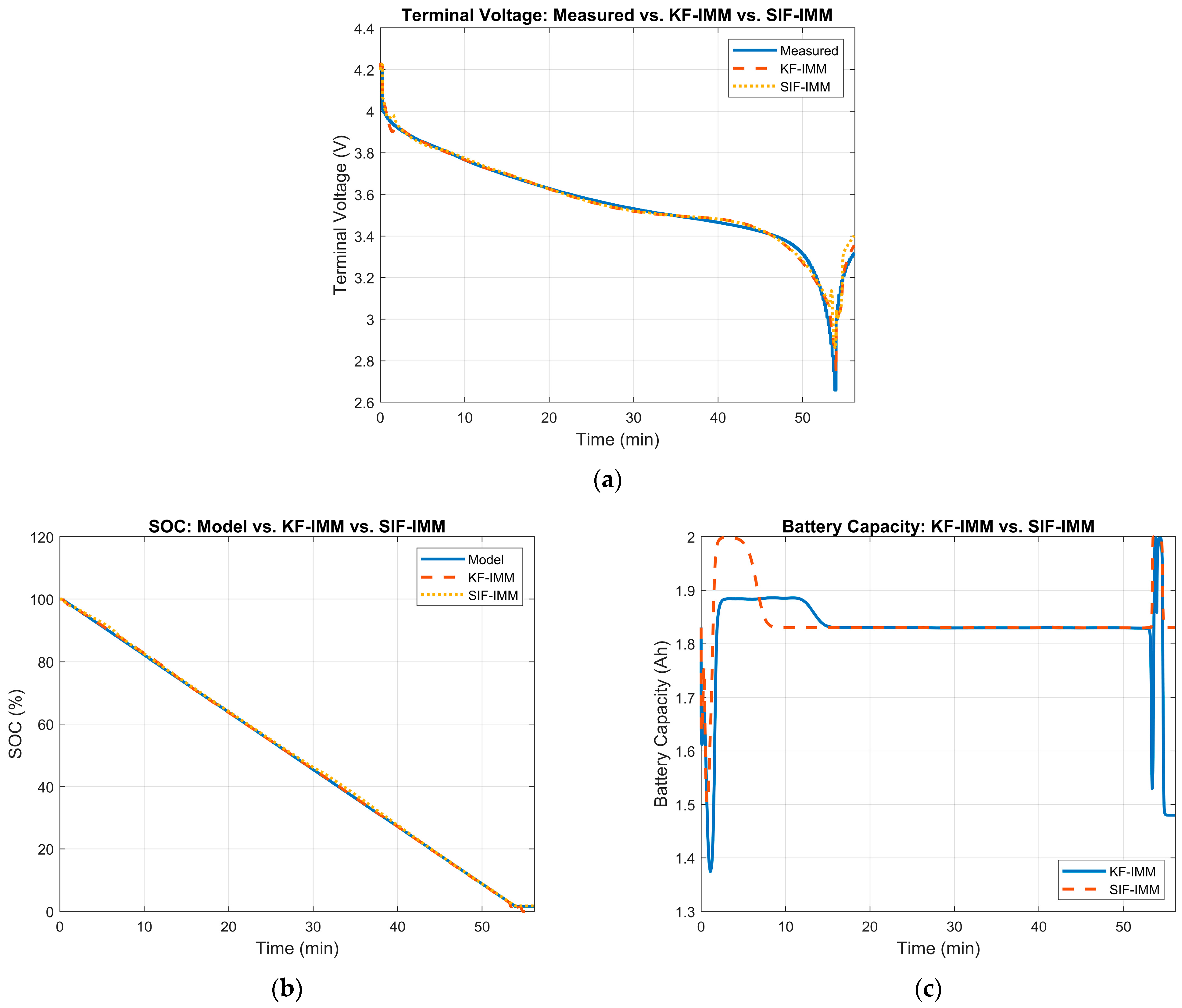
At cycle 106, the battery’s measured capacity is ~1.81 Ah. Therefore, the KF-IMM and SIF-IMM should select, for the most part, the 75% SOH mode to better match the current state of the battery. Figure 13 illustrates the estimation results of the KF-IMM and SIF-IMM. Part (a) shows the terminal voltage estimation. Part (b) depicts the SOC estimation and part (c) illustrates the battery capacity estimation at the 106th cycle.

Figure 13.
(a) Measured terminal voltage vs. KF-IMM and SIF-IMM estimation at cycle 106. (b) KF-IMM and SIF-IMM SOC estimation at cycle 106. (c) KF-IMM and SIF-IMM battery capacity estimation at cycle 106.
The terminal voltage’s RMSE values for the KF-IMM and SIF-IMM were 0.0249 and 0.0255, respectively; both of these values show strong accuracy. Furthermore, both SOC estimation results showed a good profile. Moreover, the estimated battery capacity for both algorithms remained, for the most part, at ~1.83 Ah.
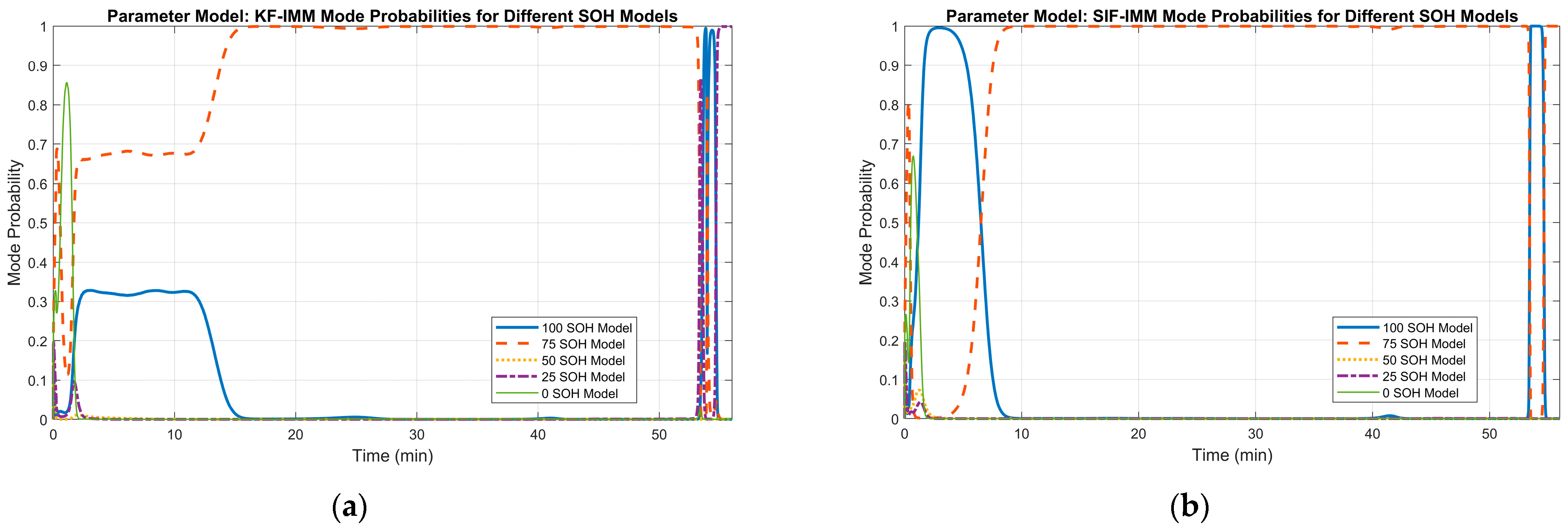
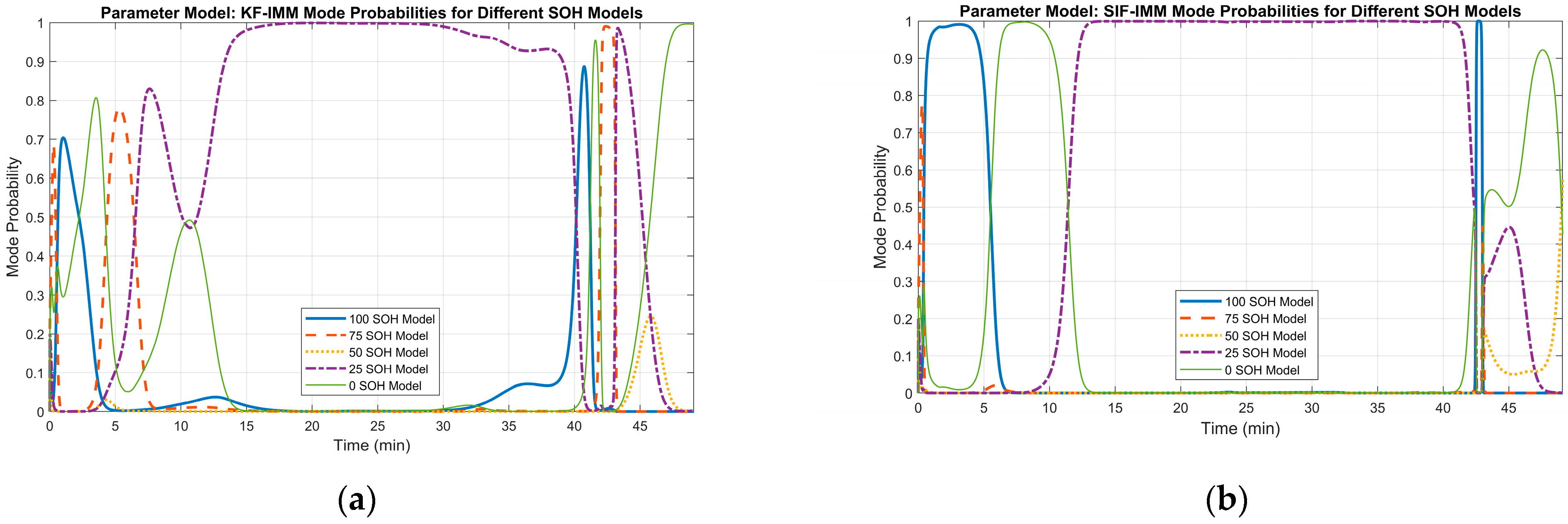
Lastly, Figure 14 illustrates the mode probability of each algorithm at cycle 106. Both algorithms switch between various modes to account for the sudden drop in voltage at the beginning of the discharge process. This switching can also be observed when the current is cut off, and the battery starts to recover after a period of ~53 min. Most importantly, it is evident that both filters select the 75% SOH mode as the better match, which reflects the measured battery capacity in the B005 dataset.
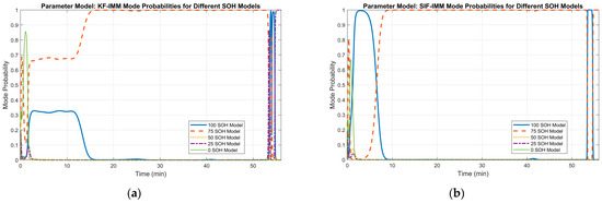
Figure 14.
(a) KF-IMM mode probability at cycle 106. (b) SIF-IMM mode probability at cycle 106.
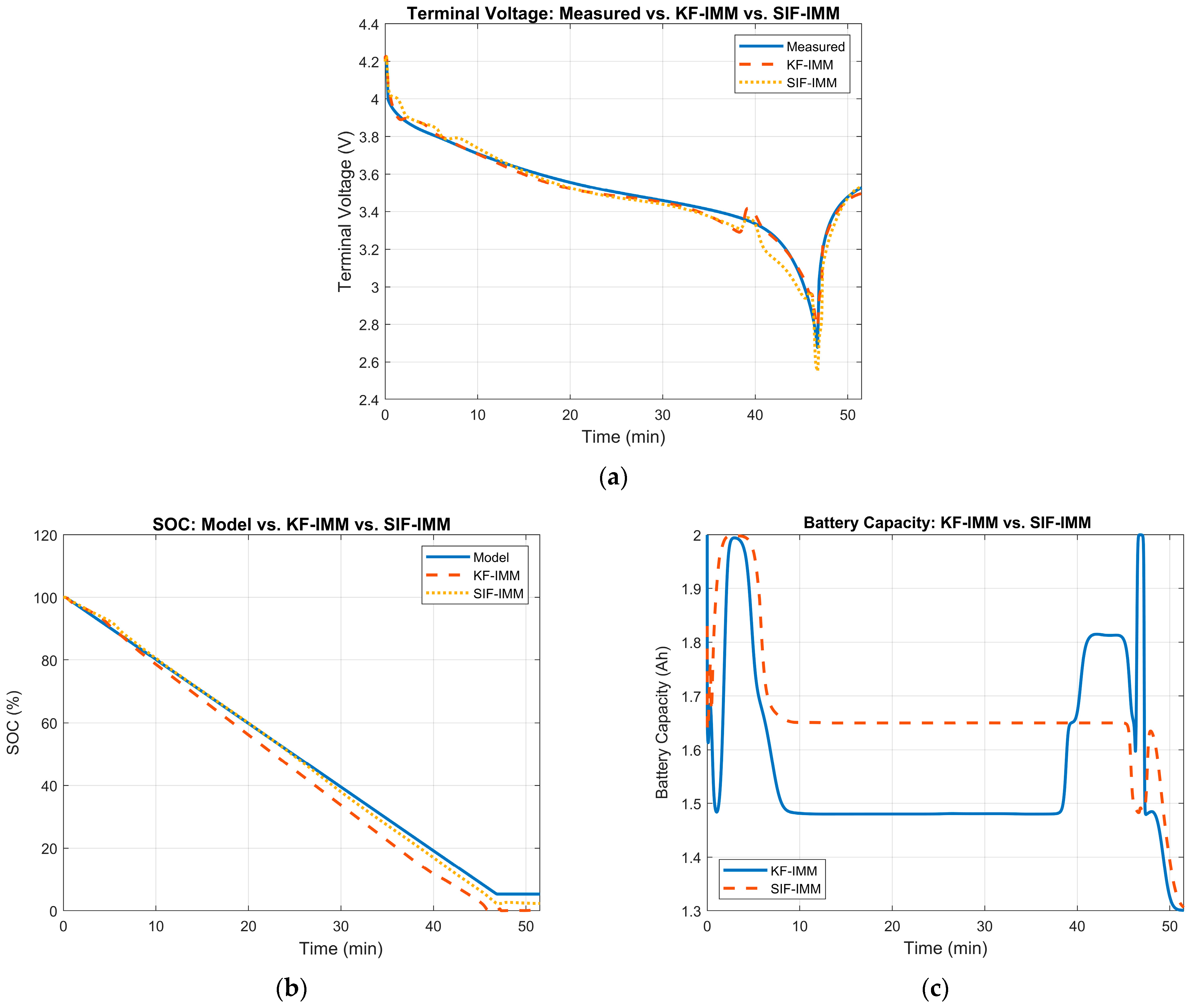
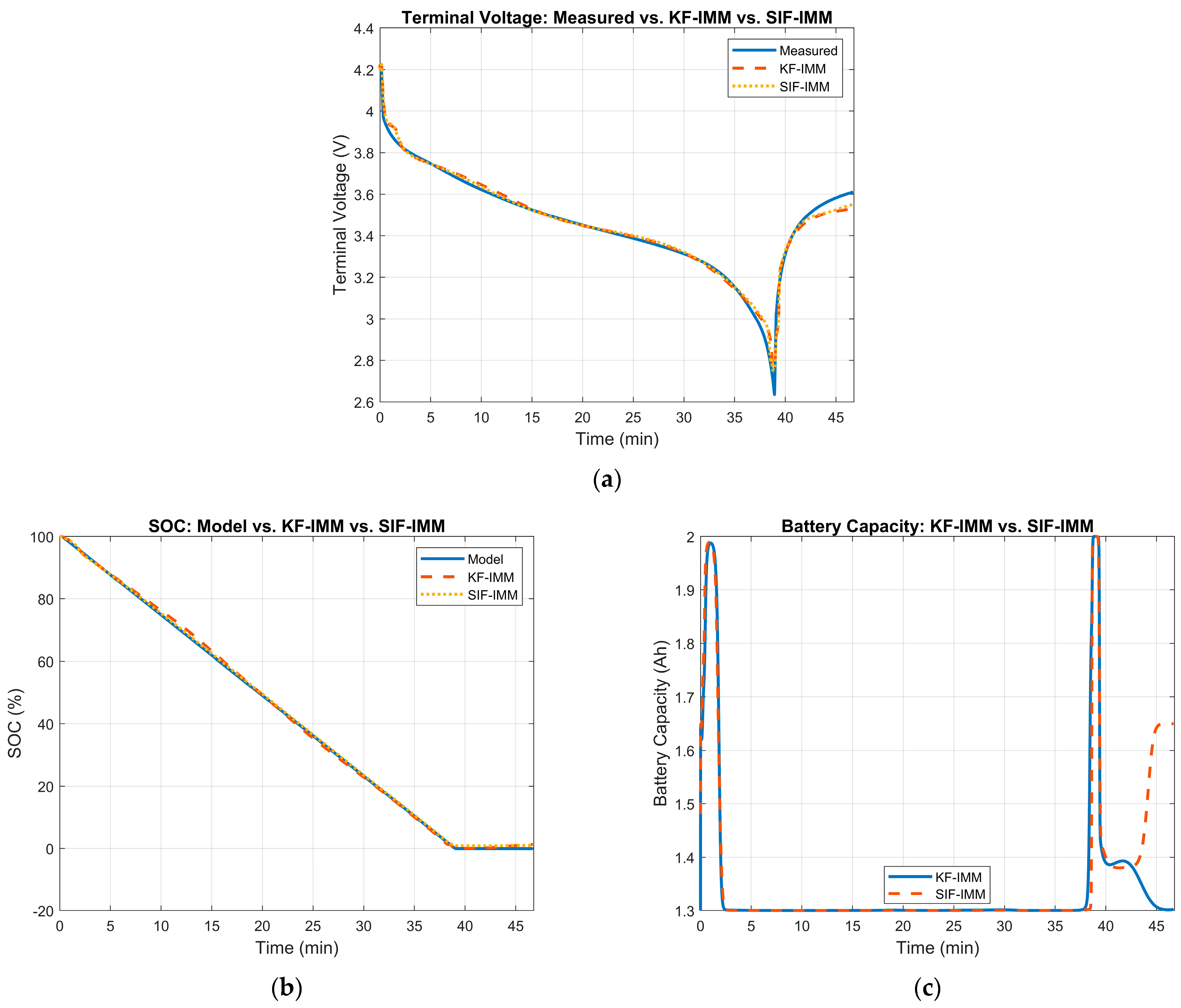
At cycle 278, the battery’s measured capacity is ~1.56 Ah. Therefore, the KF-IMM and SIF-IMM should select, for the most part, the 50% SOH mode. Figure 15 illustrates the terminal voltage, SOC, and battery capacity estimation results of the KF-IMM and SIF-IMM at the 278th cycle.
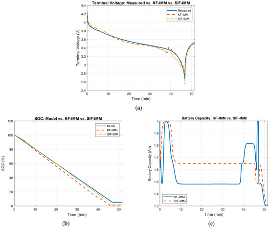
Figure 15.
(a) Measured terminal voltage vs. KF-IMM and SIF-IMM estimation at cycle 278. (b) KF-IMM and SIF-IMM SOC estimation at cycle 278. (c) KF-IMM and SIF-IMM battery capacity estimation at cycle 278.
The terminal voltage’s RMSE values for the KF-IMM and SIF-IMM were 0.0377 and 0.0257, respectively; both values suggest high accuracy. Furthermore, both SOC estimation results showed a good constant discharge profile, with the KF-IMM fully discharging the battery. In terms of battery capacity estimates, the KF-IMM had a mean value of 1.56 Ah, which matches the measured value from the dataset. The SIF-IMM has a higher mean value at 1.65 Ah. This higher value in battery capacity enforces the discrepancy in the SOC discharge profiles between both algorithms.
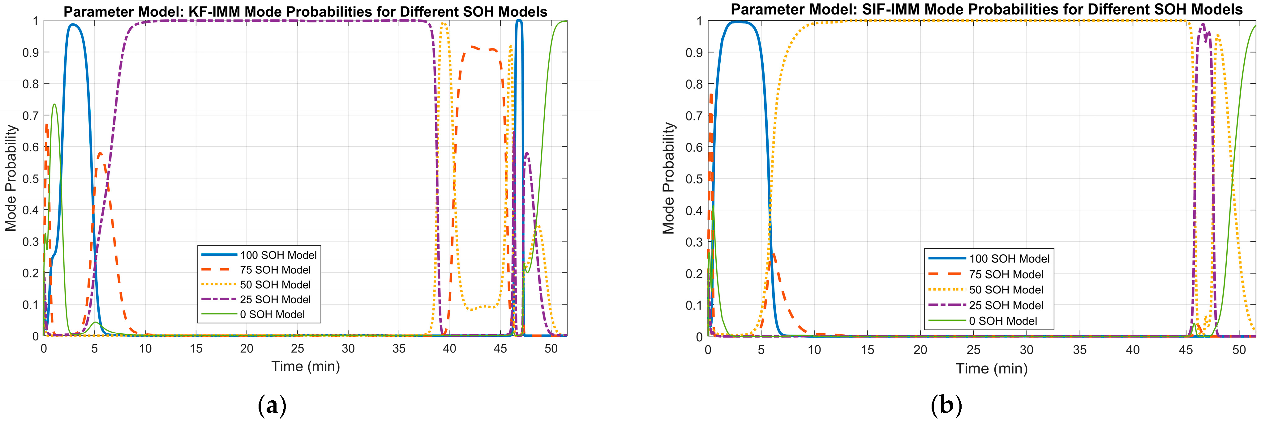
Figure 16 demonstrates the mode probability of each algorithm at cycle 278. In part (a), the KF-IMM selects the 25% SOH model as the predominant mode for most of the cycle. Looking at the same window of time in part (b) of Figure 15, the lower battery capacity allows for a faster discharge rate, which is more advantageous towards the end of the cycle when compared to the SIF-IMM results. However, the sudden jump in voltage near the 40 min mark, and the selection of the 75% SOH mode afterwards, can be a consequence of the selection of the 25% SOH mode.
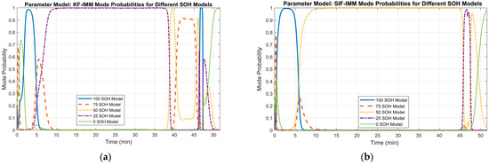
Figure 16.
(a) KF-IMM mode probability at cycle 278. (b) SIF-IMM mode probability at cycle 278.
On the other hand, the SIF-IMM method chooses the 50% SOH mode for most of the cycle. This mode selection reflects a better estimate of the current SOH of the battery based on the measured battery capacity.
At cycle 411, the battery’s measured capacity is ~1.42 Ah. Therefore, the KF-IMM and SIF-IMM should select, for the most part, the 25% SOH mode to match the current state of the battery. The estimation results of the KF-IMM and SIF-IMM are shown in Figure 17. Part (a) shows the terminal voltage results. Part (b) depicts the SOC estimation and part (c) illustrates the battery capacity estimation at the 411th cycle.
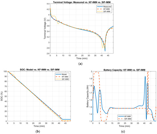
Figure 17.
(a) Measured terminal voltage vs. KF-IMM and SIF-IMM estimation at cycle 411. (b) KF-IMM and SIF-IMM SOC estimation at cycle 411. (c) KF-IMM and SIF-IMM battery capacity estimation at cycle 411.
The terminal voltage’s RMSE values for the KF-IMM and SIF-IMM were 0.0373 and 0.0239, respectively, confirming their accuracy. In part (b), both SOC estimation curves have a good overall profile that reflects a full discharge of the battery. Moreover, in terms of battery capacity, the mean value for both algorithms was ~1.51 Ah. These values are close to the measured value of 1.42 Ah in the dataset. The corresponding mode probabilities for this case are shown in Figure 18.
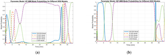
Figure 18.
(a) KF-IMM mode probability at cycle 411. (b) SIF-IMM mode probability at cycle 411.
At cycle 596, the battery’s measured capacity is ~1.3 Ah. Therefore, the KF-IMM and SIF-IMM should select, for the most part, the 0% SOH mode. Figure 19 illustrates the estimation results of the KF-IMM and SIF-IMM. Part (a) shows the terminal voltage estimation. Part (b) depicts the SOC estimation and part (c) illustrates the battery capacity estimation at the 596th cycle.
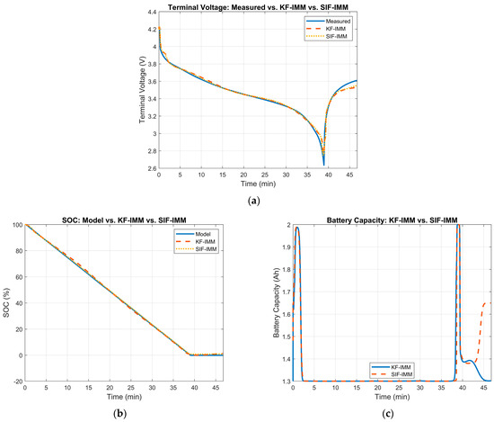
Figure 19.
(a) Measured terminal voltage vs. KF-IMM and SIF-IMM estimation at cycle 596. (b) KF-IMM and SIF-IMM SOC estimation at cycle 596. (c) KF-IMM and SIF-IMM battery capacity estimation at cycle 596.
The terminal voltage’s RMSE values for the KF-IMM and SIF-IMM were 0.0311 and 0.0251, respectively; both values show strong accuracy. Both algorithms’ SOC curves show a good full discharge profile. Moreover, the estimated battery capacity for both algorithms remained, for the most part, at ~1.33 Ah.
The mode probability of each algorithm at cycle 596 is shown in Figure 20. Both algorithms select the correct mode, which reflects the current SOH of the battery in the B005 dataset.

Figure 20.
(a) KF-IMM mode probability at cycle 596. (b) SIF-IMM mode probability at cycle 596.
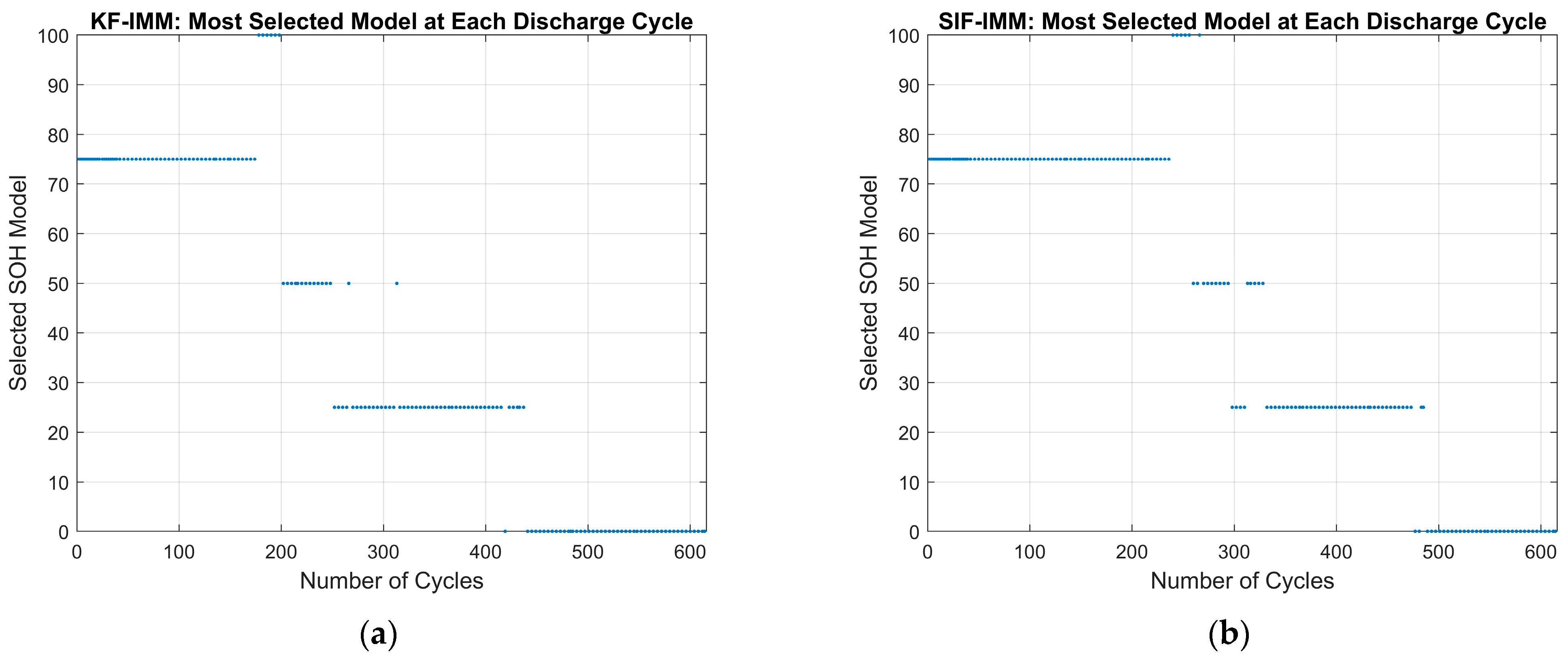
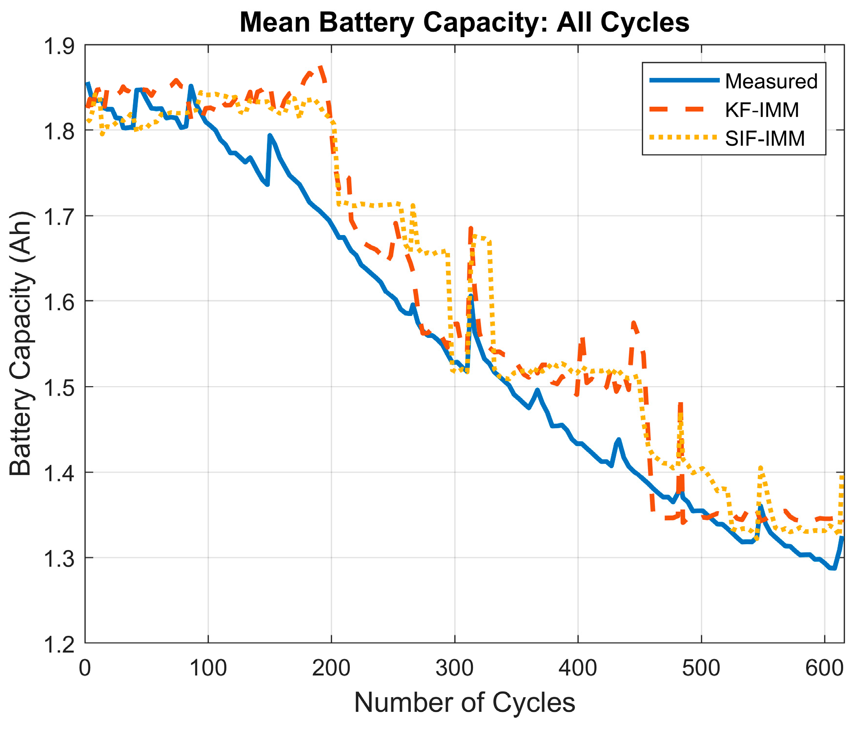
To analyze the overall estimation results of the KF-IMM and SIF-IMM, the mean battery capacity for each cycle was generated, and the mode chosen by the IMM-selected models was taken at the end of each cycle. Figure 21 shows the most frequently selected mode for each cycle. Part (a) depicts the most-selected mode of the KF-IMM and part (b) illustrates the most-selected mode of the SIF-IMM. Figure 22 depicts the mean battery capacity of both algorithms for each cycle compared to the measured battery capacity.
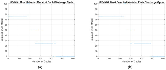
Figure 21.
(a) KF-IMM’s most selected model for each cycle. (b) SIF-IMM’s most selected model for each cycle.

Figure 22.
Mean battery capacity across all cycles.
From Figure 21 it is evident that neither algorithm made use of the 100% SOH model at the beginning of the experiment. The reason is evident if one were to look at the starting capacity of the battery, which is closer to the 75% SOH model. Based on the break points for each identified SOH region, the algorithms should ideally switch between modes after cycles 98, 225, 375, and 588. Since the battery’s capacity starts at 75% SOH, the first switch should occur after the 225th cycle. However, the KF-IMM switches to the 50% SOH model earlier than the SIF-IMM. This early jump reinforces the results from Figure 15 and Figure 16. Furthermore, neither algorithm makes consistent use of the 50% SOH model and both algorithms make an early jump to the 25% SOH model. Finally, both algorithms switch to the 0% SOH model before the expected 588th cycle. Taking a holistic view on Figure 21, both algorithms show the desired downward step trend.
It can be seen from Figure 22 that both algorithms show a good battery capacity trend. The battery capacity RMSE values for the KF-IMM and SIF-IMM were 0.060 and 0.065, respectively. When compared to the difference between the healthy and retired battery capacity values, the RMSE values correspond to an error of ~9% in determining the current SOH of the battery. After further inspection of Figure 22, the early switches between modes at cycles ~190 and ~440 can be justified.
7. Conclusions
This paper presented a strategy that utilizes the interacting multiple model (IMM) algorithm integrated with the Kalman filter (KF) and sliding innovation filter (SIF) methods for mode-matched filtering. As demonstrated by the results, the proposed strategy accurately estimates the state of charge (SOC) and state of health (SOH) of a lithium-ion battery (LiB) under cycling conditions. More specifically, the KF-based methods worked more accurately under ‘normal’ operating conditions (e.g., when the dynamic models closely resembled the actual operating models). However, when the SOH started to reduce or the battery began to degrade (essentially when there was model mismatch), the SIF-based methods yielded better estimates.
In the proposed strategy, the IMM is used to track the correct battery capacity, thus estimating the SOH of the battery. Meanwhile, the KF and SIF are used to estimate the SOC of the battery during cycling. The integration of these algorithms with the IMM resulted in strategies called KF-IMM and SIF-IMM. Moreover, the proposed strategy was evaluated using experimental data and was found to be successful in tracking the SOH of the battery. In the future, the proposed strategy will be implemented on a real-world BMS for further testing and verification. Lastly, this strategy has the potential to be used for predicting battery retirement, the results of which will be explored further in future studies.
Author Contributions
Investigation, R.B. and S.A.G.; writing—original draft preparation, R.B.; writing—review and editing, S.A.G., M.B., M.A. and S.M. All authors have read and agreed to the published version of the manuscript.
Funding
This research received no external funding.
Data Availability Statement
Publicly available datasets were analyzed in this study. The B005 dataset can be found here: https://ti.arc.nasa.gov/tech/dash/groups/pcoe/prognostic-data-repository/, accessed on 20 August 2022. B. Saha and K. Goebel (2007). The “Battery Data Set” is provided by the NASA Ames Prognostics Data Repository (http://ti.arc.nasa.gov/project/prognostic-data-repository, accessed on 20 August 2022), NASA Ames Research Center, Moffett Field, CA.
Conflicts of Interest
The authors declare no conflict of interest.
Appendix A
In the proposed strategy, the IMM is used to track the correct battery capacity, thus estimating the SOH of the battery. Meanwhile, the KF and SIF are used to estimate the SOC of the battery during cycling. The integration of these algorithms with the IMM resulted in strategies referred to as KF-IMM and SIF-IMM. The following figure helps further illustrate the overall architecture of the proposed strategies.
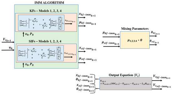
Figure A1.
Overall architecture of IMM-KF and IMM-SIF strategies.
Figure A1.
Overall architecture of IMM-KF and IMM-SIF strategies.
References
- Ren, G.; Ma, G.; Cong, N. Review of Electrical Energy Storage System for Vehicular Applications. Renew. Sustain. Energy Rev. 2015, 41, 225–236. [Google Scholar] [CrossRef]
- Thackeray, M.M.; Wolverton, C.; Isaacs, E.D. Electrical Energy Storage for Transportation—Approaching the Limits of, and Going beyond, Lithium-Ion Batteries. Energy Environ. Sci. 2012, 5, 7854. [Google Scholar] [CrossRef]
- Lu, L.; Han, X.; Li, J.; Hua, J.; Ouyang, M. A Review on the Key Issues for Lithium-Ion Battery Management in Electric Vehicles. J. Power Sources 2013, 226, 272–288. [Google Scholar] [CrossRef]
- Zhang, S.; Sun, H.; Lyu, C. A Method of SOC Estimation for Power Li-Ion Batteries Based on Equivalent Circuit Model and Extended Kalman Filter. In Proceedings of the 2018 13th IEEE Conference on Industrial Electronics and Applications (ICIEA), Wuhan, China, 31 May–2 June 2018; IEEE: Piscataway, NJ, USA, 2018; pp. 2683–2687. [Google Scholar]
- Vidal, C.; Malysz, P.; Kollmeyer, P.; Emadi, A. Machine Learning Applied to Electrified Vehicle Battery State of Charge and State of Health Estimation: State-of-the-Art. IEEE Access 2020, 8, 52796–52814. [Google Scholar] [CrossRef]
- Meddings, N.; Heinrich, M.; Overney, F.; Lee, J.-S.; Ruiz, V.; Napolitano, E.; Seitz, S.; Hinds, G.; Raccichini, R.; Gaberšček, M.; et al. Application of electrochemical impedance spectroscopy to commercial Li-ion cells: A review. J. Power Sources 2020, 480, 228742. [Google Scholar] [CrossRef]
- Zhang, R.; Li, X.; Sun, C.; Yang, S.; Tian, Y.; Tian, J. State of Charge and Temperature Joint Estimation Based on Ultrasonic Reflection Waves for Lithium-Ion Battery Applications. Batteries 2023, 9, 335. [Google Scholar] [CrossRef]
- Kandepu, R.; Foss, B.; Imsland, L. Applying the Unscented Kalman Filter for Nonlinear State Estimation. J. Process Control 2008, 18, 753–768. [Google Scholar] [CrossRef]
- Partovibakhsh, M.; Liu, G. An Adaptive Unscented Kalman Filtering Approach for Online Estimation of Model Parameters and State-of-Charge of Lithium-Ion Batteries for Autonomous Mobile Robots. IEEE Trans. Control Syst. Technol. 2015, 23, 357–363. [Google Scholar] [CrossRef]
- Yadkuri, F.F.; Khosrowjerdi, M.J. Methods for Improving the Linearization Problem of Extended Kalman Filter. J. Intell. Robot. Syst. 2015, 78, 485–497. [Google Scholar] [CrossRef]
- Sanjurjo, E.; Naya, M.Á.; Blanco-Claraco, J.L.; Torres-Moreno, J.L.; Giménez-Fernández, A. Accuracy and Efficiency Comparison of Various Nonlinear Kalman Filters Applied to Multibody Models. Nonlinear Dyn. 2017, 88, 1935–1951. [Google Scholar] [CrossRef]
- Foletto, T.C.; Moreno, U.F.; Lopes, A.M. Comparison of Packet Loss Compensation in Nonlinear Networked Control Systems Using the Methods Extended Kalman Filter and Unscented Kalman Filter. In Proceedings of the ETFA2011, Toulouse, France, 5–9 September 2011; IEEE: Piscataway, NJ, USA, 2011; pp. 1–7. [Google Scholar]
- Yi, S.; Zorzi, M. Robust fixed-lag smoothing under model perturbations. J. Frankl. Inst. 2023, 360, 458–483. [Google Scholar] [CrossRef]
- Wang, D.; Huang, H.; Tang, Z.; Zhang, Q.; Yang, B.; Zhang, B. A Lithium-Ion Battery Electrochemical–Thermal Model for a Wide Temperature Range Applications. Electrochim. Acta 2020, 362, 137118. [Google Scholar] [CrossRef]
- Tang, S.-X.; Camacho-Solorio, L.; Wang, Y.; Krstic, M. State-of-Charge Estimation from a Thermal–Electrochemical Model of Lithium-Ion Batteries. Automatica 2017, 83, 206–219. [Google Scholar] [CrossRef]
- Ghalkhani, M.; Bahiraei, F.; Nazri, G.-A.; Saif, M. Electrochemical–Thermal Model of Pouch-Type Lithium-Ion Batteries. Electrochim. Acta 2017, 247, 569–587. [Google Scholar] [CrossRef]
- Wang, L.; Niu, J.; Zhao, W.; Li, G.; Zhao, X. Study on Electrochemical and Thermal Characteristics of Lithium-Ion Battery Using the Electrochemical-Thermal Coupled Model. Int. J. Energy Res. 2019, 43, 2086–2107. [Google Scholar] [CrossRef]
- Barcellona, S.; Piegari, L. Lithium Ion Battery Models and Parameter Identification Techniques. Energies 2017, 10, 2007. [Google Scholar] [CrossRef]
- Zhang, X.; Zhang, W.; Lei, G. A Review of Li-Ion Battery Equivalent Circuit Models. Trans. Electr. Electron. Mater. 2016, 17, 311–316. [Google Scholar] [CrossRef]
- Davide, A. Battery Management Systems for Large Lithium-Ion Battery Packs; Artech: Morristown, NJ, USA, 2010. [Google Scholar]
- Marcicki, J.; Onori, S.; Rizzoni, G. Nonlinear Fault Detection and Isolation for a Lithium-Ion Battery Management System. In Proceedings of the ASME 2010 Dynamic Systems and Control Conference, Cambridge, MA, USA, 1 January 2010; ASMEDC: New York, NY, USA, 2010; Volume 1, pp. 607–614. [Google Scholar]
- Meng, J.; Yue, M.; Diallo, D. A Degradation Empirical-Model-Free Battery End-Of-Life Prediction Framework Based on Gaussian Process Regression and Kalman Filter. IEEE Trans. Transp. Electrif. 2022, 9, 4898–4908. [Google Scholar] [CrossRef]
- Xu, J.; Sun, C.; Ni, Y.; Lyu, C.; Wu, C.; Zhang, H.; Yang, Q.; Feng, F. Fast Identification of Micro-Health Parameters for Retired Batteries Based on a Simplified P2D Model by Using Padé Approximation. Batteries 2023, 9, 64. [Google Scholar] [CrossRef]
- Singh, A.; Izadian, A.; Anwar, S. Nonlinear Model Based Fault Detection of Lithium Ion Battery Using Multiple Model Adaptive Estimation. IFAC Proc. Vol. 2014, 47, 8546–8551. [Google Scholar] [CrossRef]
- Xia, X.; Wei, Y. Lithium-Ion Batteries State-of-Charge Estimation Based on Interactive Multiple-Model Extended Kalman Filter. In Proceedings of the 2016 22nd International Conference on Automation and Computing (ICAC), Colchester, UK, 7–8 September 2016; IEEE: Piscataway, NJ, USA, 2016; pp. 204–207. [Google Scholar]
- Singh, A.; Izadian, A.; Anwar, S. Fault Diagnosis of Li-Ion Batteries Using Multiple-Model Adaptive Estimation. In Proceedings of the IECON 2013—39th Annual Conference of the IEEE Industrial Electronics Society, Vienna, Austria, 10–13 November 2013; IEEE: Piscataway, NJ, USA, 2013; pp. 3524–3529. [Google Scholar]
- Bustos, R. State of Health Estimation of Lithium-Ion Batteries Using Dual Filters and the IMM Strategy. Ph.D. Thesis, University of Guelph, Guelph, ON, Canada, 2022. [Google Scholar]
- Hasib, S.A.; Islam, S.; Chakrabortty, R.K.; Ryan, M.J.; Saha, D.K.; Ahamed, M.H.; Moyeen, S.I.; Das, S.K.; Ali, M.F.; Islam, M.R.; et al. A Comprehensive Review of Available Battery Datasets, RUL Prediction Approaches, and Advanced Battery Management. IEEE Access 2021, 9, 86166–86193. [Google Scholar] [CrossRef]
- Tian, N.; Wang, Y.; Chen, J.; Fang, H. On Parameter Identification of an Equivalent Circuit Model for Lithium-Ion Batteries. In Proceedings of the 2017 IEEE Conference on Control Technology and Applications (CCTA), Mauna Lani Resort, HI, USA, 27–30 August 2017; IEEE: Piscataway, NJ, USA, 2017; pp. 187–192. [Google Scholar]
- Kalman, R.E. A New Approach to Linear Filtering and Prediction Problems. J. Basic Eng. Mar 1960, 82, 35–45. [Google Scholar] [CrossRef]
- Gadsden, S.A.; Habibi, S.; Kirubarajan, T. Kalman and Smooth Variable Structure Filters for Robust Estimation. IEEE Trans. Aerosp. Electron. Syst. 2014, 50, 1038–1050. [Google Scholar] [CrossRef]
- Gadsden, S.A.; Al-Shabi, M. The Sliding Innovation Filter. IEEE Access 2020, 8, 96129–96138. [Google Scholar] [CrossRef]
- Bustos, R.; Gadsden, S.A.; Al-Shabi, M.; Mahmud, S. Lithium-Ion Battery Health Estimation Using an Adaptive Dual Interacting Model Algorithm for Electric Vehicles. Appl. Sci. 2023, 13, 1132. [Google Scholar] [CrossRef]
- Wei, X.; Yimin, M.; Feng, Z. Lithium-Ion Battery Modeling and State of Charge Estimation. Integr. Ferroelectr. 2019, 200, 59–72. [Google Scholar] [CrossRef]
Disclaimer/Publisher’s Note: The statements, opinions and data contained in all publications are solely those of the individual author(s) and contributor(s) and not of MDPI and/or the editor(s). MDPI and/or the editor(s) disclaim responsibility for any injury to people or property resulting from any ideas, methods, instructions or products referred to in the content. |
© 2024 by the authors. Licensee MDPI, Basel, Switzerland. This article is an open access article distributed under the terms and conditions of the Creative Commons Attribution (CC BY) license (https://creativecommons.org/licenses/by/4.0/).

