Investigating the Impact of Agricultural, Financial, Economic, and Political Factors on Oil Forward Prices and Volatility: A SHAP Analysis

Abstract

Accurately forecasting crude oil prices is crucial due to its vital role in the industrial economy. In this study, we explored the multifaceted impact of various financial, economic, and political factors on the forecasting of crude oil forward prices and volatility. We used various machine learning models to forecast oil forward prices and volatility based on their superior predictive power. Furthermore, we employed the SHAP framework to analyze individual features to identify their contributions in terms of the prediction. According to our findings, factors contributing to oil forward prices and volatility can be summarized into four key focal outcomes. First, it was confirmed that soybean forward pricing overwhelmingly contributes to oil forward pricing predictions. Second, the SSEC is the second-largest contributor to oil forward pricing predictions, surpassing the contributions of the S&P 500 or oil volatility. Third, the contribution of oil forward prices is the highest in predicting oil volatility. Lastly, the contribution of the DXY significantly influences both oil forward price and volatility predictions, with a particularly notable impact on oil volatility predictions. In summary, through the SHAP framework, we identified that soybean forward prices, the SSEC, oil volatility, and the DXY are the primary contributors to oil forward price predictions, while oil forward prices, the S&P 500, and the DXY are the main contributors to oil volatility predictions. These research findings provide valuable insights into the most-influential factors for predicting oil forward prices and oil volatility, laying the foundation for informed investment decisions and robust risk-management strategies.

1. Introduction

Crude oil is an indispensable energy source for the development of the industrial economy and is also a strategic resource for countries (Guo et al. [1]). Consequently, forecasting oil prices is an important and challenging issue because many economic and non-economic factors influence these prices. For example, economic growth, political events, and psychological expectations affect oil prices. Crude oil price forecasting has become an important, challenging affair in recent decades (Safari and Davallou [2]). The impact of oil price changes on the real economy and financial markets has been investigated extensively (Baumeister and Peersman [3]; Hamilton [4]; Hamilton [5]; Jones and Kaul [6]; Kilian [7]; Kilian and Park [8]). In addition, oil prices are helpful predictors of the direction of stock returns on many markets (Pönkä [9]). They are commonly used predictors, such as in 3-month interest rates, dividend yields, and lagged stock returns (Rapach et al. [10]). Therefore, the accurate forecasting of crude oil prices has important implications, particularly for policymakers and investors’ risk management and investment portfolios (Chai et al. [11]; Wang et al. [12]).

Furthermore, significant changes in crude oil prices have always caused panics in the global economy. In general, a leap in crude oil prices would result in inflation and a recession in oil-consuming nations, negatively impacting the global economy. A sharp drop in oil prices hinders the economic development of oil-producing countries and causes political and social unrest (Gholamian et al. [13]; Chen and Hsu [14]). Therefore, the accurate prediction of crude oil prices is essential for stable and rapid economic development (Chen et al. [15]).

Scholars have recently conducted extensive research on oil price predictions. Crude-oil-price-forecasting models can be classified into two main categories: econometric and artificial (Zhao et al. [16]). In the past few decades, methods based on traditional statistical and econometric techniques, such as the autoregressive integrated moving average (ARIMA) model (Yu et al. [17]), the generalized autoregressive conditional heteroscedasticity (GARCH) model (Hou and Suardi [18]), and the vector autoregressive regression (VAR) model (Mirmirani and Li [19]), have been widely applied to crude oil price forecasting. However, these models may be insufficient for obtaining the nonlinear features of crude oil prices (Safari and Davallou [2]). To overcome this limitation, nonlinear and emerging artificial intelligence methods, such as artificial neural networks (Jammazi and Aloui [20]), support vector machines (Yu et al. [21]), and long short-term memory (Wu et al. [22]), provide solutions for the nonlinear crude oil price predictions.

Neural network models have clear advantages in capturing nonlinearity and demonstrate superior predictive capabilities compared to traditional models (Belkin et al. [23]). Nonetheless, they suffer from a notable drawback: they lack the ability to elucidate the rationale behind specific predictions or decisions. In order to tackle this issue, researchers are actively working on the development of methodologies such as explainable AI (XAI), which aims to enhance the transparency and interpretability of machine learning models.

This study aims to assess the extent to which various contributing factors influence the prediction of crude oil forward prices and volatility. To achieve this objective, we gathered a comprehensive set of assets and financial, economic, and political variables known to exert an influence on crude oil price dynamics. Specifically, agricultural commodities were employed to represent assets, while stock price indices were utilized as the financial factors. Additionally, economic policy uncertainty (EPU) and geopolitical risk (GPR) indices were employed to capture economic and political impacts, as evidenced by previous research. Further insights into the relationship between these variables and the oil market are provided in Section 2.1, where the details of the relevant studies are outlined.

We propose the following hypotheses based on the existing literature:

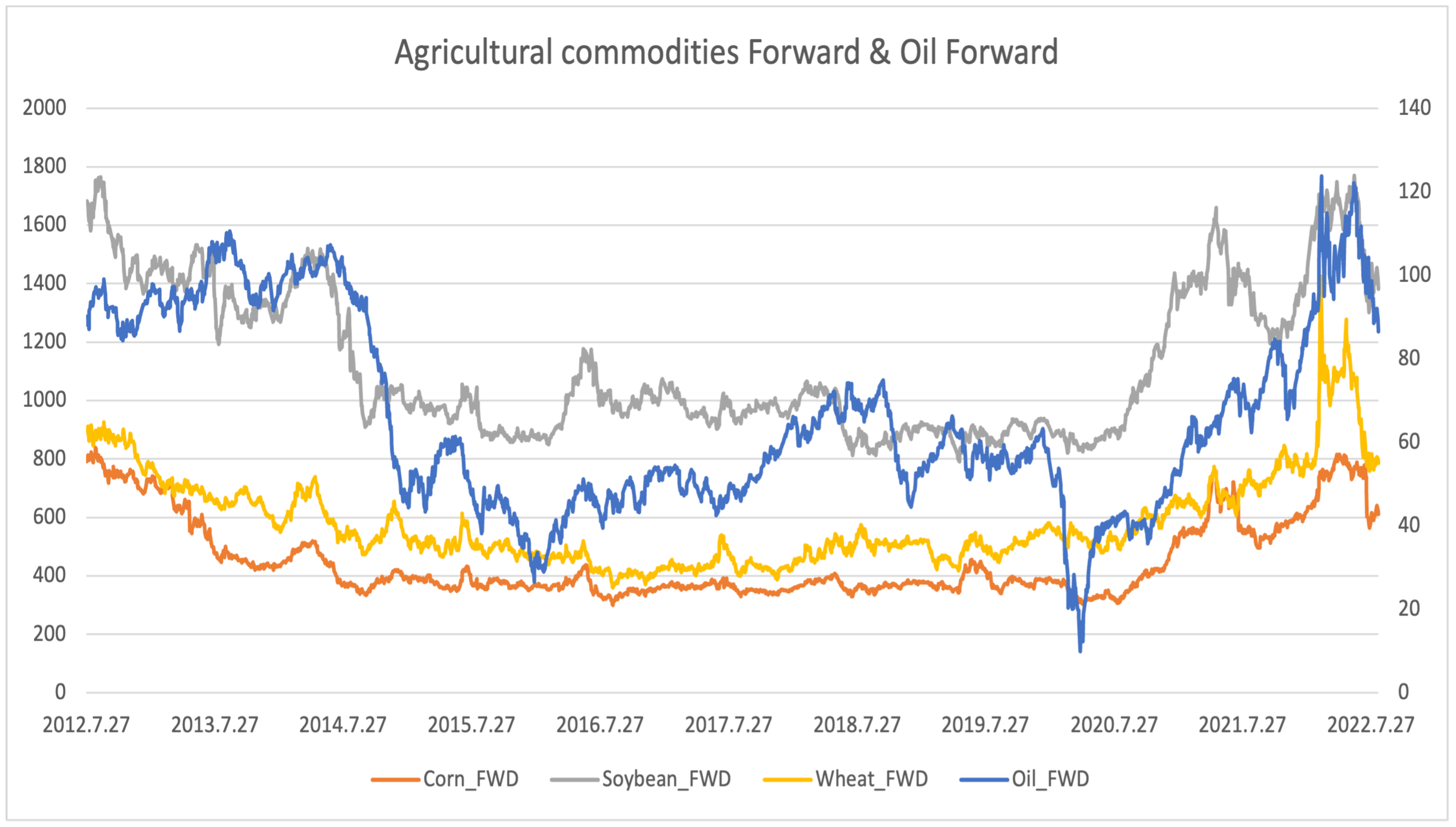
• The relationship between the crude oil market and agricultural commodities is tightly interdependent. Agricultural crops, which can be used to produce biodiesel as a substitute for crude oil, also affect crude oil demand.
• The relationship between the crude oil market and stock indices, like the S&P 500, is remarkable. Stock indices serve as economic indicators, and fluctuations in stock prices directly affect the crude oil market due to the changing demand associated with economic cycles.
• There is a notable connection between the crude oil market and currency exchange rates, notably concerning the U.S. Dollar index (DXY). The U.S. Dollar, as the global reserve currency and primary medium of exchange for international oil transactions, plays a pivotal role in influencing both crude oil prices and currency exchange rates.
• There exists an evident relationship between crude oil prices and EPU. Changes in EPU may also influence crude oil prices through the impact on investor sentiment and risk perceptions.
• The relationship between crude oil prices and GPR is noticeable. Geopolitical tensions in major oil-producing regions can directly impact crude oil prices by disrupting supply chains, limiting production capacity or creating uncertainty about future supplies.

In terms of methodology, we utilized machine learning algorithms and the Shapley additive explanation (SHAP) framework to examine the significant features of the relationship between oil and the various above-mentioned factors. As mentioned earlier, machine learning methodologies perform well regarding their predictive power, and SHAP is a recently developed XAI model that helps interpret and explain the predictions of machine learning models. By applying SHAP to interpret the machine learning model’s forecasting results, we obtained more-accurate and -interpretable insights into the forecasting factors that drive the prediction of oil forward prices and volatility. Recently, many studies have utilized various combined machine learning algorithms and SHAP (Jabeur et al. [24], Sarp et al. [25], Homafar et al. [26], Li [27], Yang et al. [28], Fatahi et al. [29], Farzipour et al. [30], Stef et al. [31], Mao et al. [32], Yang et al. [33]).

In this study, our workflow involved predicting oil forward prices and oil volatility using a range of machine learning algorithms and employing SHAP (to do this, we used the Pycaret (3.0.2) and SHAP packages in Python.). To enhance the accuracy and reliability of our predictions, we applied the SHAP framework to only machine learning models with excellent predictive performance. By doing this, we can strengthen the robustness of both our prediction results and the SHAP analysis outcomes. This helped us validate the effectiveness of our machine learning algorithms in predicting oil forward prices and volatility while providing insights into the key drivers of these predictions.

The contributions of this study are twofold. First, although many recent studies have focused on oil prediction using machine learning models, we employed the SHAP model, which solves the black-box problem of machine learning, to analyze the predictions. Second, we compared oil forward price and volatility forecasts simultaneously. Previous studies usually only predicted one of the oil’s prices, forward or volatility. However, this study sheds light on the differences between oil forward prices and volatility by analyzing their predictive performance altogether. Third, through the comparative analysis of crude oil forward prices and various determinants of volatility, this study identifies the primary factors influencing the prediction outcomes. Distinct from conventional approaches, our methodology not only achieves superior prediction accuracy leveraging machine learning models, but also employs explainable artificial intelligence (XAI) techniques to quantify their respective contributions to predictive efficacy. This research, thus, makes a substantive contribution to the extant literature by presenting empirical findings that enhance our understanding of the predictive mechanisms.

The remainder of this paper is organized as follows. The following section briefly reviews previous studies on oil forecasting. Section 3 describes the oil and the other data set. In addition, the research design and methodologies are explained in Section 4. Section 5 presents the empirical results and discussion. Finally, Section 6 presents the summary and concluding remarks.

2. Literature Review

This section provides an overview of research investigating the relationship between crude oil and various market factors, as well as previous studies focused on forecasting crude oil prices.

2.1. Oil and Various Factors

Numerous prior investigations have established a robust relationship between the prices and volatilities of oil and agricultural commodities (Baffes [34]; Nazlioglu et al. [35]; Wang et al. [36]; Rezitis [37]; Paris [38]; Yip et al. [39]; Naeem et al. [40]; Sun et al. [41]; Tiwari et al. [42]). According to such studies, crude oil prices have shown a positive correlation with the commodity market in normal circumstances, unless there is a specific oil shock or economic event occurring. In particular, Naeem et al. [40] investigated the spillover effects of uncertainty between oil and various commodity markets. It focuses on the causal impact of global factors on these spillovers, particularly during the global financial crisis of 2008–2009. The authors discovered a significant bi-directional interaction between the oil and agriculture markets, with this interaction becoming notably more intense during periods of turmoil.

Previous studies have demonstrated the relevance between oil prices and various stock markets. Specifically, investigations have been conducted on the impact of oil shocks on the American and Chinese stock markets (Wei et al. [43]; Cong et al. [44]; Li and Wei [45]; Degiannakis et al. [46]; Sakaki [47]; Wei et al. [48]). Studies suggest that the causal effect between the oil market and the stock market significantly depends on whether the research is conducted using stock market indices, sector indices, or corporation data and on whether the stock market operates in a net oil-importing or net oil-exporting country, as well as whether it is over a long-term or short-term period. For instance, Degiannakis et al. [46] investigated whether the American stock market and oil prices show the same directional movement. They discussed how oil price volatility transmits to stock market volatility and how the performance of the stock market supports the prediction of oil prices and oil price volatility. Sakaki [47] confirmed that positive shocks to American oil production and economic activities result in higher stock returns and a positive influence when investigating the supply and demand of oil affecting the stock market. Similarly, there is a body of literature examining the influence of oil prices on European and Japanese stock markets (Arouri et al. [49]; Bagirov and Mateus [50]; Joo and Park [51]; Broadstock et al. [52]; Ding et al. [53]). These studies highlight the importance of understanding the relationship between oil prices and stock markets for effective portfolio management and the influence of external factors like geopolitical and financial crises on market performance. Katsampoxakis et al. [54] studied the interrelations between stock returns and crude oil prices for European oil-producing and -importing countries using a vector autoregression (VAR) model to estimate the stock market responses to changes in oil prices. The study showed that there is no interdependence in steady periods, but the causality from stock markets to oil prices increases in highly volatile periods.

In the realm of currencies, research has predominantly focused on investigating the correlation between gold prices, industrial production, and oil (Peersman and Van Robays [55]; Samanta and Zadeh [56]; Malliaris and Malliaris [57]; Arfaoui and Ben Rejeb [58]; Sun et al. [59]; Donkor et al. [60]). Results across these findings reveal intricate interdependencies and multifaceted relationships between oil prices, stock markets, gold prices, and USD exchange rates. These studies collectively highlight the complexity of global financial markets, demonstrating how various factors and economic variables interact with and influence each other across different periods and economic conditions. For example, Samanta and Zadeh [56] investigated the interdependence of economic variables such as gold prices, the dollar exchange rate, the dollar index, oil prices, and the American stock index over more than two decades. Using techniques like cointegration and Granger causality analysis, the study suggests that there are long-term co-movements among these variables, albeit with small spillover indices. Similarly, Sun et al. [59] examined the complex interplay between U.S. monetary policy, the U.S. Dollar index, and WTI crude oil prices. They investigated cross-correlations and their multifractal features over time, identifying significant impacts of U.S. monetary policy on the interconnectedness of these markets.

About EPU, several studies have explored its impact on the oil market and industry (Aloui et al. [61]; Gu et al. [62]; Ilyas et al. [63]; Qin et al. [64]). These studies demonstrated that both EPU and the oil market have varying effects, ranging from negative to positive, on market dynamics. These impacts are more pronounced in certain contexts, such as in oil-producing countries and during periods of high policy uncertainty. Additionally, GPR, another political index, has been the subject of studies measuring its predictive power and impact on oil prices and oil volatility (Gu et al. [62]; Liu et al. [65]; Huang et al. [66]; Qian et al. [67]). Findings have shown the significant influence of GPR on oil market volatility, rather than directly on returns, with its effect being particularly pronounced through volatility jumps post-financial crisis and during recessions. These studies indicate the utility of GPR, including serious geopolitical events, as critical for forecasting future oil market fluctuations, offering valuable insights for investors, policymakers, and risk-management strategies.

2.2. Econometric Methods

Numerous studies have focused on forecasting the price and volatility of crude oil by employing various economic models. Hou and Suardi [18] conducted a comparative analysis of two distinct types of GARCH models, namely parametric GARCH models and nonparametric GARCH models, in their efforts to predict the volatility of Brent and Western Texas Intermediate (WTI) crude oil. Wang and Wu [68] employed univariate GARCH models and multivariate GARCH models to make predictions regarding the price and volatility of WTI crude oil, along with gasoline, jet fuel, and heating oil. Their findings indicated that multivariate GARCH models outperformed their univariate counterparts in forecasting price, whereas univariate GARCH models proved superior in forecasting volatility.

Wen et al. [69] analyzed the presence of structural breaks in the volatility of WTI crude oil futures using sixteen heterogeneous autoregressive (HAR)-type volatility models. Their investigation revealed the existence of structural breaks and a leverage effect, with the HAR-RSV and HAR-CJ models exhibiting the best forecasting performance among the HAR-type models. Charles and Darné [70] examined the volatility of WTI and Brent crude oil, taking into account the presence of jumps. Their predictive modeling encompassed the GARCH, GJR-GARCH, EGARCH, GAS, and MSM models for raw returns of WTI and Brent crude oil. The results indicated that asymmetric models, such as GARCH, GJR-GARCH, and EGARCH, outperformed the GARCH-, GAS-type, and BMSM models.

Moving forward, Nademi and Nademi [71] utilized a semiparametric Markov switching model to predict the prices of WTI crude oil, Brent, and OPEC. Among the various models tested, including AR, MA, ARIMA, and EGARCH, the non-parametric model demonstrated superior predictive power. Lin et al. [72] applied uni-regime GARCH-type models with a Markov or Hidden Markov framework to the Daqing oil market, ultimately identifying the EGARCH model as a robust performer. Moreover, the Hidden Markov-EGARCH model emerged as a reliable predictor of crude oil price volatility.

Finally, Scarcioffolo and Etienne [73] analyzed price volatility patterns in WTI crude oil and Henry Hub natural gas, employing a Markov-switching GARCH (MS-GARCH) model and other GARCH-type models to capture regime switches in commodity volatility. Their findings favored the MS-GARCH model as the most-effective in capturing the series of volatility changes.

Table 1. The review summary for the previous studies using the econometric methodologies.

Study	Method	Advantages	Limitations	Data Requirements
Hou and Suardi [18]	GARCH	Volatility Clustering Forecasting Volatility Flexibility	Assumption of Normal Distribution Stationary Requirement Computational Intensity	Financial Time Series Data Return Series Stationary Time-Series
Wen et al. [69]	HAR	Captures Long Memory Simple Structure Ease of Interpretation	Assumption of Linearity Volatility Forecasting Sensitivity to Measurement Error	Financial Time Series Data Volatility Series Aggregated Time Horizons
Charles and Darné [70]  Nademi and Nademi [71]  Lin et al. [72]	EGARCH	Leverage Effect No Restriction on Parameters Robust to Large Shocks	Complexity Sensitivity to Outliers Forecasting Horizon	Return Series Data Stationary Time Series High-Frequency Data

presents a summary outlining the advantages, limitations, and data requirements of the econometric methodology in the studies mentioned earlier.

2.3. Machine Learning Methods

In addition to econometric models, various machine learning methodologies have also been employed in studies aimed at predicting oil prices. Xie et al. [74] utilized support vector machines (SVM) to forecast crude oil prices, relying on the spot price of WTI. Zhang et al. [75] employed a combined ensemble empirical mode decomposition (EEMD), Least-Squares support vector machine (LSSVM), and GARCH to provide forecasts for daily, weekly, and monthly WTI crude oil prices. The work of Yu et al. [21] demonstrated that SVM-based predictions for one-step-ahead monthly WTI crude oil spot prices and Brent crude oil spot prices outperformed traditional time series forecasts like ARIMA. Zhang and Hamori [76] proposed a new method to forecast downturns in the U.S. crude oil futures market. They compared machine learning techniques like random forests, Logistic Regression, support vector machines, and XGBoost, finding XGBoost most effective, with an 86% detection rate using a fixed-length moving window. Moreover, the application of long short-term memory (LSTM) and EEMD in daily WTI crude oil price prediction revealed that the combination of LSTM and EEMD yielded superior results compared to using a standalone LSTM model (Wu et al. [22]). Manowska and Bluszcz [77] also introduced an innovative model for forecasting crude oil consumption in Poland, utilizing LSTM networks. They assessed the model’s accuracy with various coefficients, highlighting the potential of LSTM in enhancing predictive analytics in the energy sector.

Furthermore, Zhang et al. [78] adopted variational modal decomposition (VMD) to segment time series data, employing sample entropy (SE) in conjunction with gated recurrent units (GRUs) for forecasting WTI crude oil prices spanning the period from 2010 to 2019. Their findings underscored that this deep learning framework exhibited enhanced accuracy and explanatory power in comparison to traditional methods for oil price prediction. Luo et al. [79] presented a groundbreaking approach using Convolutional Neural Networks (CNNs) for forecasting short-term crude oil futures prices. The authors, through meticulous comparison with benchmark models, demonstrated the superior accuracy of CNNs in handling the complex, nonlinear characteristics of oil price movements.

In summation, many econometric models and machine learning approaches have been applied to the prediction of oil prices and volatility. Notably, recent research has shown that machine learning models often surpass traditional models in terms of predictive performance (Yu et al. [21]; Kim et al. [80]; Shobana and Umamaheswari [81]; Xu et al. [82]). Consequently, our study also exploits machine learning algorithms to forecast oil futures and gauge oil volatility.

Table 2. The review summary for the previous studies using the machine learning algorithms.

Study	Method	Advantages	Limitations	Data Requirements
Xie et al. [74]	SVM	High-Dimensional Spaces Memory Efficiency Versatility	Kernel Models Scalability Output Interpretability	Numerical Data
Wu et al. [22], Kim et al. [80]	LSTM	Long-Term Dependencies Flexibility Handling Sequential Data	Complexity Training Time Tuning	Sequential Data
Zhang et al. [78]	VMD	Mode Decomposition Adaptation Noise Robustness	Parameter Selection Computational Complexity Application Specificity	Time Series Data
Luo et al. [79]	CNNs	Excellent for Image Data Feature Learning Versatility	Computational Intensity Overfitting Interpretability	Transformed into Embeddings
Zhang and Hamori [76]	XGBoost	High Performance Efficiency Feature Importance	Parameter Tuning Overfitting High-Dimensional Sparse Data	Numerical, Categorical Data

provides a summary outlining the advantages, limitations, and data requirements of the machine learning algorithms in the studies mentioned in this subsection.

3. Data and Research Design

3.1. Data Description

In our research, we extensively employed a diverse array of financial data classes, encompassing commodities, foreign exchange, stock indices, volatility, U.S. economic policy uncertainty (US EPU), and the geopolitical risk index (GPR) to investigate their impact on oil forward and volatility. Additionally, within each of these classes, we integrated multiple datasets to facilitate a comprehensive analysis.

To begin, we first focused on forward price and volatility measures for major agricultural commodities, specifically oil, corn, wheat, and soybean. Figure 1 presents each collected forward index. The indices for agricultural commodities utilized in this study were derived from the Chicago Board Options Exchange (CBOE) and the Chicago Board of Trade (CBOT). Subsequently, we turned our attention to stock market indices from three distinct countries and regions: the United States, China, Japan, and the European Union, illustrated in Figure 2. To further diversify our dataset and enhance the robustness of our research, we incorporated foreign exchange data from both the United States and the European Union. The Dollar index and Euro index were used in our research, also presented in Figure 3. Finally, we examined the contributions of economic risk posed by political uncertainty and geopolitical tensions using the U.S. economic policy uncertainty (US EPU) and the geopolitical index (GPR). These economic and politic indices are also exhibited in Figure 4, followed by the previous graph of the indices (Figure 1, Figure 2 and Figure 3) we mentioned. All the data utilized in our study were collected over the period from 27 July 2012 to 16 August 2022, with meticulous attention to addressing any gaps in the data through careful removal. The primary sources for these datasets were the Refinitiv Datastream of Reuters and Investing.com (accessed on 1 January 2023).

Table 3. Descriptive statistics for daily financial datasets in research.

Sectors	Asset	Mean	Max.	Min.	Std. Dev.	Skewness	Kurtosis
Forward	Oil	66.12	123.7	−37.63	22.81	0.39	−0.74
	Corn	451.64	838.75	301.5	133.69	1.30	0.43
	Soybean	1128.74	1769	791	254.58	0.71	−0.82
	Wheat	583.20	1425.25	361	156.40	1.50	2.69
Volatility index	Oil	37.38	325.15	14.5	20.10	4.99	42.35
Stock index	S&P 500	2646.95	4793.54	1353.33	878.54	0.76	−0.37
	Eurostoxx50	3330.66	4401.49	2263.36	415.72	0.10	−0.14
	Nikkei225	20,095.27	30,670.1	8534.12	5115.39	−0.04	−0.43
	SSEC	2975.47	5166.35	1950.01	559.66	0.08	0.40
Currency	DXY	92.62	108.54	78.85	6.90	−0.62	−0.60
	Euro index	97.18	113.19	84.4	7.49	0.47	−0.78
Risk factors	US EPU	121.84	861.1	3.32	97.68	2.68	10.05
	GPR	109.54	542.66	14.36	52.03	2.45	11.66

presents the summary statistics for oil forward prices/volatility and the forecasting factors. Among agricultural commodities, soybean forward prices exhibited the largest mean and standard deviation, while wheat and corn demonstrated a higher asymmetric distribution than soybean and oil. Notably, wheat displayed the highest skewness and kurtosis. Turning to stock indices, the Nikkei displayed the highest mean and standard deviation. The S&P 500 exhibited slight skewness compared to the other stock indices. As for U.S. EPU and GPR, both indices demonstrated high skewness and kurtosis.

3.2. Research Design

In this research, we leveraged a variety of machine learning methodologies to project oil forward prices and assess oil volatility, taking into account a range of agricultural, financial, economic, and political factors. Specifically, we utilized forward price index data from three agricultural commodities, four distinct stock indices, two foreign exchange indices, the EPU index, and the GPR index to formulate predictions for both oil forward prices and oil volatility. To gauge the influence of the factors on the forecasting of oil forward prices and volatility, we employed the SHAP framework to evaluate their individual contributions. In this analytical framework, we used oil forward prices and oil volatility as benchmarks, allowing us to systematically compare the relative impacts of the various factors on the prediction accuracy of both oil forward prices and oil volatility.

Furthermore, we employed multiple machine learning methodologies to forecast both of them. Through forecasting performance evaluation among the machine learning methods, we selected several machine learning methodologies in terms of forecasting performance. The selected methodologies then underwent a hyperparameter optimization process to enhance their performance. Subsequently, we utilized the optimized machine learning methodologies to predict oil forward prices and volatility, respectively. Finally, we applied the SHAP framework to the prediction results, allowing us to evaluate the contribution of these communities in the forecasting process. Figure 5 displays the research design of this study.

This research process offers several advantages. First, it enabled us to select an outstanding prediction methodology from a pool of diverse machine learning methods. As the dominant machine learning methodologies differ based on the specific prediction target, it is crucial to carefully consider and choose the most-suitable methodology among various candidates. Second, by comparing the results of the SHAP framework for the selected machine learning methodologies, we enhanced the robustness of our findings. This comparative analysis provides additional insights into the contribution of the diverse factors, strengthening the overall validity of our research.

In this study, we mainly used the “Pycaret” python framework to forecast the oil price and volatility based on the research design explained in the previous section. Pycaret is an open-source Python framework for streamlining the machine learning process. It simplifies tasks such as data preparation, model training, hyperparameter tuning, model selection, and interpretation, according to the workflow in Figure 5. As the first process, we compared the various machine learning models in terms of forecasting performance, and

Table 4. The error measures for oil forward prediction. Notes: MAE = mean absolute error; MSE = mean-squared error; RMSE = root-mean-squared error.

Model	MAE	MSE	RMSE	R2
Random Forest	2.1813	13.7509	3.6809	0.9731
Light Gradient Boosting Machine	2.5674	15.385	3.8857	0.9699
Extreme Gradient Boosting	2.5484	15.6656	3.9277	0.9693
K Neighbors	2.8626	25.6515	5.0456	0.9496
Decision Tree	2.6412	26.0652	5.0633	0.9489
Gradient Boosting	3.793	28.4029	5.3058	0.9444
AdaBoost	6.4469	62.8457	7.9245	0.8763
Bayesian Ridge	8.4772	113.112	10.6054	0.7785
Linear Regression	8.4906	113.114	10.6055	0.7784

and

Table 5. The error measures for oil volatility prediction.

Model	MAE	MSE	RMSE	R2
Random Forest	2.4417	28.1812	4.9049	0.9426
Extreme Gradient Boosting	2.7017	29.3377	5.055	0.9382
Gradient Boosting	3.9056	40.1237	6.1372	0.9079
Light Gradient Boosting Machine	2.8973	44.591	6.0797	0.9117
Decision Tree	3.0093	46.4475	6.4154	0.899
K Neighbors	3.3234	48.0869	6.5249	0.8972
AdaBoost	8.3166	112.596	10.5284	0.7118
Least Angle	8.3092	212.7261	14.2385	0.5115
Bayesian Ridge	8.288	212.7279	14.2352	0.5119

display the forecasting performance of various methods. According to the forecasting results, we selected three machine learning algorithms, XGBoost, LightGBM, and random forest, that perform well in common with oil forward price prediction results and oil volatility prediction results. The following subsections briefly review the three machine learning methods.

Initially, we assessed various machine learning models for their forecasting performance. Table 4 and Table 5 present the results of this comparison. Based on these findings, we identified three machine learning algorithms—XGBoost, LightGBM, and random forest—that consistently performed well in both oil price and volatility predictions. In the following subsections, we provide brief overviews of these three machine learning methods.

4. Machine Learning and SHAP

4.1. Machine Learning Models

In this subsection, we briefly review the top three machine learning algorithms mentioned above.

4.1.1. Extreme Gradient Boosting (XGBoost)

The gradient boosting model is an ensemble machine learning algorithm that combines multiple weak learners to create strong ones. A notable advancement in this field is Extreme Gradient Boosting (XGBoost), introduced by Chen and Guestrin [83]. XGBoost overcomes the limitations of traditional Gradient Boosting Machines (GBMs) by addressing computational constraints, handling regularization, enabling parallel training, and effectively managing missing data. Additionally, XGBoost incorporates a second-order Taylor expansion in its loss function, in contrast to the GBM’s first-order Taylor expansion. A fundamental concept in the XGBoost algorithm is the interconnection between the current training set and previous learning outcomes, assigning weights to each sample in every iteration. Several studies provide evidence that XGBoost is a highly accurate and flexible predictor in various applications (Feng et al. [84]; Nasiri et al. [85]; Alsahaf et al. [86]). Compared to conventional machine learning approaches, XGBoost offers a broader range of hyperparameters, allowing for better tuning and superior performance. Notably, in previous studies on oil price forecasting, the XGBoost model has demonstrated superior performance compared to conventional econometric methodologies (Guliyev and Mustafayev [87]; Tissaoui et al. [88]; Khalfaoui et al. [89]).

4.1.2. LightGBM

The Light Gradient Boosting Machine (LightGBM), proposed by Ke et al. [90], is an ensemble machine learning model that improves upon the GBM. The GBM yields unsatisfactory results when dealing with datasets containing numerous features and large data sizes, mainly due to its exhaustive scanning of all instances and features. XGBoost mitigates this issue by employing a histogram-based algorithm that reduces the computation time while maintaining accuracy. In contrast, LightGBM achieves computational efficiency through two novel algorithms: Gradient-based One-Side Sampling (GOSS) and exclusive feature bundling (EFB).

In the case of GOSS, each instance has gradients that influence the training error based on their values. GOSS retains instances with high gradients while applying random sampling to those with small gradients, effectively reducing the number of instances and expediting computation. Data with high dimensions are often sparse, and EFB addresses this by transforming bundles of features into single features. EFB converts bundles created by greedy bundling algorithms, which are formed based on variables with conflicting counts, into a unified variable.

When comparing XGBoost and LightGBM, it becomes evident that LightGBM significantly accelerates processing while maintaining similar accuracy to XGBoost (Al Daoud [91]).

4.1.3. Random Forest

Random forest, introduced by Breiman [92], is an ensemble machine learning model based on decision trees. A decision tree is a machine learning algorithm that uses rules to classify and regress feature data. Random forest is a specialized application of decision trees using a technique called bagging. Bagging involves sampling random features with replacements to create independent training datasets. In random forest, each tree can be prone to overfitting, and the variables chosen may introduce bias into the distribution. However, by randomly selecting predictor variables through bagging, an optimized model is created by averaging the results from multiple independent training datasets. Random input also helps reduce computational load during tree construction.

There are two main reasons for using bagging in random forest. First, it randomizes the selection of variables, which can improve accuracy. Second, it makes use of Out-Of-Bag (OOB) data to reduce generalization errors. OOB data include variables other than the randomly chosen predictor variables. Random forest also calculates feature importance; if a feature is not used in the final tree model, it is considered less important. Rodriguez-Galiano et al. [93] argued that random forest exhibits higher accuracy and model stability than other machine learning algorithms and artificial neural networks in certain situations.

4.2. SHAP Framework

The Shapley value of game theory has been extensively utilized to reasonably measure each player’s contribution and distribute the total benefit (Shapley [94]). Game theory can be divided into cooperative and noncooperative games, and the Shapley value is contained in cooperative games, which shows that players cooperate with each other and assemble coalitions to maximize total profit (Bloch and Friedrich [95]; Dong et al. [96]; Rozemberczki and Sarkar [97]).

The Shapley value has four useful properties: efficiency, symmetry, dummy, and additivity (Li [27]). Efficiency demands that the total feature contributions sum up symmetrically, which refers to the requirement that two features that contribute equally to the prediction have the same Shapley values. The dummy property indicates that a feature with a marginal contribution of zero to all possible models has a null Shapley value. Additivity demonstrates the solution’s fairness and uniqueness if all four properties are satisfied Shapley [94].

The Shapley value examines the weighted sum of players’ marginal contributions in a cooperative game. When p players participate in a cooperative game, let S be a subset containing $\left|S\right|$ players (1), where $|·|$ is the number of elements in the subset S. Suppose that ${\varphi }_i$ is a contribution function of the ith player, which represents the value of coalition S and the total expected sum of profits obtained by the cooperation of the members of S. Except for the ith player, the set of variables is denoted by P. For example, ${\varphi }_i$ is defined as

$${\varphi }_i=\sum _{S\subseteq \{x_1,...,x_p\}\setminus x_i}\frac{\left|S\right|!\left(\right|P|-|S|-1)!}{\left|P\right|!}[f(S\cup x_i)-f\left(S\right)],$$

(1)

where $f\left(S\right)$ is the outcome of the game when a player in subset S participates.

The Shapley value was also adopted to evaluate the global significance of the features in interpretable machine learning recently. In XAI, features are considered players, and the prediction is the total benefit (Aas et al. [98]). Lundberg and Lee [99] introduced the Shapley additive explanation (SHAP), which is a unified framework for explaining predictions. SHAP decomposes the black-box model $f\left(x\right)$ into a simpler additive model (2).

$$g\left(z^{\prime }\right)={\varphi }_0+\sum _{i=1}^d{\varphi }_i{z}_i^{\prime }$$

(2)

where $z^{\prime }\in {\{0,1\}}^d$ and d is the number of simplified features. Here, ${\varphi }_i$ denotes the Shapley value obtained from (1). ${\varphi }_0$ is constant when all inputs are missing.

5. Empirical Results and Discussion

5.1. Empirical Results

In this section, we present the results of the oil forward price and volatility predictions using three selected machine learning models. Additionally, we conducted an analysis of the forecasting outcomes using the SHAP framework.

We first enhanced the performance of the three chosen machine learning models through hyperparameter tuning. Subsequently, we utilized these tuned models to predict both oil forward prices and oil volatility. The forecasting outcomes are presented in

Table 6. The prediction results of the tuned models.

	Oil Forward Price				Oil Volatility
Model	MAE	MSE	RMSE	R2	MAE	MSE	RMSE	R2
Random Forest	1.1445	3.3493	1.8301	0.9933	1.6547	7.0638	2.6578	0.9194
LightGBM	0.8344	1.9783	1.4065	0.9961	1.0628	4.4600	2.1119	0.9491
XGBoost	0.9878	2.6332	1.6227	0.9948	1.0819	3.6257	1.9041	0.9587

, offering a comprehensive overview of the results achieved. Furthermore, Figure 6 graphically depicts the forecasted oil forward prices and volatility alongside their corresponding actual values based on the three tuned machine learning algorithms. According to the empirical findings presented in both the table and the figure, we show the compelling performance of the top three models in terms of the oil forward price and oil volatility prediction. Moreover, it is noteworthy that the differences in the prediction errors among these models were not significant.

The soybean forward prices emerged as the most-impactful factor affecting oil forward prices, with their influence further magnified by the elevated soybean forward price values. This substantial impact can be attributed to the inherent connection between soybean and crude oil, wherein soybean serves as the primary raw material for the production of soybean biodiesel. These significant findings will be expounded upon in the subsequent section of our discussion. Furthermore, the SHAP analysis conducted across the three machine learning models revealed a positive correlation between soybean forward prices and oil forward prices. Specifically, an increase in the price of soybean forwards corresponds to a rise in oil forward prices, while a decrease in the price of soybean forwards corresponds to a decline in oil forward prices.

The second-most-influential factor affecting oil forward prices is the SSEC, a representative stock index in China. Our SHAP analysis revealed two notable findings. Firstly, the SSEC demonstrated a negative correlation with oil forward prices, indicating that the price of SSEC negatively impacts the prediction of oil forward prices. At the point of a zero SHAP value, the relationship exhibits a mixed aspect with both negative and positive plots, gradually transitioning into a positive correlation as the SSEC values decrease. Secondly, the impact of the SSEC is more substantial than that of the S&P 500. Notably, the influence of the SSEC is more than twice as significant as the impact of the S&P 500. Additionally, the S&P 500 tends to exhibit a positive correlation with oil forward prices, in contrast to the negative correlation observed with the SSEC. Further elucidation of these findings will be provided in the subsequent section of our analysis.

Research has long explored the connection between the Chinese stock market and the oil market. Li et al. [100] found a one-way causality from sector-specific stock prices to oil prices during December 2005 to June 2007, indicating that fluctuations in Chinese sectoral stock prices can predict oil price shifts. This underscores China’s significant influence on global oil markets. Factors such as China’s economic influence, oil consumption, and speculative stock market activities contribute to this relationship. Wen et al. [101] further confirmed the impact of China’s stock market on oil prices, showing that changes in sectors like agriculture, mining, and manufacturing can forecast oil price changes. This suggests that Chinese market activities and investor sentiments can affect global oil prices, highlighting China’s role as a major oil consumer and importer.

A notable outcome derived from the SHAP analysis pertains to the influence of the DXY. Despite the incorporation of various financial datasets, the impact of the DXY ranked as the second-highest, irrespective of the consideration of agricultural commodities and oil volatility. The SHAP analysis of the DXY yielded a distinctive result among the indices, revealing an unusual pattern, where higher values of the DXY led to zero impact on the SHAP value. However, beyond the interval around the zero impact, the influence exhibited a dynamic pattern in the positive section, fluctuating as the DXY values decreased, increased, and decreased again, while still maintaining a positive impact. Further exploration and discussion of this intriguing phenomenon will be undertaken in the subsequent section of our analysis.

When forecasting oil volatility, the primary influential factor is the behavior of oil forwards, which surpasses all other features in predictive power. Additionally, it is notable that low oil forward prices contribute significantly to the occurrence of high oil volatility, as illustrated in Figure 7b,d,f and Figure 8b,d,f. This observation aligns with the well-documented leverage effect, wherein oil volatility tends to increase when oil forward values decrease (Kristoufek [102]). Furthermore, it is noteworthy that multiple studies have identified the leverage effect as a pivotal element in predicting oil volatility (Chan and Grant [103]; Yang et al. [104]; Liang et al. [105]). This body of research underscores the significance of the leverage effect in understanding and forecasting fluctuations in oil market volatility.

Consistent with the outcomes observed in oil forward forecasting, the DXY exhibited a noteworthy impact on the prediction of oil volatility. In contrast to its influence on oil forward prices, the SHAP analysis of the DXY revealed a positive correlation with oil volatility. Notably, the DXY occupied a substantial position in both the forecasting of oil forward prices and volatility, underscoring its relevance as a key determinant in the predictive models for both aspects of the oil market.

Our analysis indicates GPR has a minimal contribution to predicting oil futures and volatility. This finding appears contrary to the widely recognized notion that international disputes exert a significant impact on the crude oil market. However, existing research suggests that GPR tends to have a short-term effect on the crude oil market (Brandt and Gao [106]; Li et al. [107]; Mei et al. [108]). Given the utilization of long-term data in our study, we inferred that the influence of GPR on our results was minimal.

5.2. Discussion

In this section, we mainly discuss the relationship between soybean and crude oil. The dynamic relationship between crude oil and soybean prices can be explained through various mechanisms. Specifically, crude oil plays a pivotal role in influencing transportation costs, which, in turn, have a notable impact on the production costs associated with soybeans. Furthermore, it is noteworthy that an escalation in soybean prices has the potential to decrease the demand for soybean-based biodiesel, an energy source that relies predominantly on crude oil. The amount of soybean oil used for biodiesel production approximates half of the monthly consumption of soybean oil. Therefore, it can be predicted that the price of soybeans, which produce soybean oil, has a close price correlation with oil FWDs (Aaron M. Ates and Maria Bukowski, Oil Crops Outlook: August 2023, OCS-23h, U.S. Department of Agriculture, Economic Research Service, 15 August 2023. web https://www.ers.usda.gov/publications/pub-details/?pubid=107310, accessed on 1 January 2024). Accordingly, many studies have investigated the intricate connection between soybeans and crude oil, explaining this relationship primarily within the context of biodiesel production (Hassouneh et al. [109], Nazlioglu et al. [35], Gozgor et al. [110], Yip et al. [39], Tiwari et al. [111]).

Furthermore, an important factor that strengthens the connection between soybeans and crude oil is the climate risk. That is, rapid climate change plays a pivotal role in elucidating the price fluctuations observed in both crude oil and soybeans. Climate change directly affects crop productivity by causing extreme weather events, rising sea levels, etc. Despite advances in agricultural technology that have increased crop yields, the persistent threat of ongoing climate shifts may reduce crop productivity (Olesen and Bindi [112], Chen et al. [113], Liang et al. [114], Sarkar et al. [115]). In particular, climate change significantly harms soybean production, with rising summer temperatures causing significant disruption. According to previous studies (Mall et al. [116], Kucharik and Serbin [117]), climate-change-induced increases in summer temperatures could potentially result in a significant reduction in soybean production, estimated to be in the range of 10% to 20%. Consequently, reduced soybean yields may place upward pressure on soybean prices. Moreover, climate risk also affects the oil industry. As a strategic response to climate risk, limitations on oil consumption can indeed influence oil prices and their volatility. This phenomenon has been considered in several recent studies that examined the connection between climate policy and fluctuations for oil prices and volatility (Liang et al. [118], He and Zhang [119], Ren et al. [120], Zhou et al. [121]).

Highlighting the significance of the SSEC in the context of oil forwards, it is particularly noteworthy that the feature value of the SSEC exhibited a pronounced impact compared to the influence of the S&P 500. Specifically, both the S&P 500 and SSEC demonstrated substantial relevance, a relationship that has been previously explored in existing studies investigating the correlation between the oil market and the U.S. stock market (Sakaki [47], Wei et al. [43]). Notably, Wei et al. [43] found that the Chinese stock market, represented by the SSEC, displayed a more-pronounced negative influence than the S&P 500 in response to short-term oil price fluctuations. This phenomenon was attributed to the greater maturity of the U.S. stock market, where institutional investment holds a majority share. In contrast, the Chinese stock market is characterized by a high presence of retail investors, rendering it more susceptible to short-term oil price increases driven by speculation.

Moreover, Li and Wei [45] asserted that the financial crisis triggered a heightened dependency between the oil market and the Chinese stock market due to the risk spillover effect. Given the accelerated dependence on imported crude oil in the wake of China’s economic prosperity, crude oil holds crucial significance for both China’s real economy and the stock market. Additionally, investigations by Arfaoui and Ben Rejeb [58] and Wei et al. [48] delved into the substantial impact of oil futures prices and Chinese oil gross imports on the oil price.

In the context of oil volatility, the S&P 500 emerged as a more-impactful factor in forecasting volatility, demonstrating a positive correlation. This finding aligns with the research conducted by Sakaki [47], which investigated the influence of oil volatility on the S&P 500 market.

Our noteworthy finding from the SHAP analysis underscores the significant contribution of the DXY to both oil forwards and volatility. This observation aligns with the assertions made by Sun et al. [59], who, in the context of industry production, highlighted the pivotal role of crude oil as a crucial energy resource. The study emphasized that an increase in oil prices impacts production costs, investments, and consumers, ultimately leading to an acceleration of the inflation rate. This, in turn, results in lower interest rates and a subsequent decrease in the Dollar index.

Similarly, Arfaoui and Ben Rejeb [58] emphasized the impact of the U.S. Dollar, linking it to oil prices and gold prices within the framework of global interdependence and the financialization process. These prior studies provide support for the SHAP analysis conducted in the forecasting of oil forwards. In the realm of oil volatility, Ji and Fan [122] conducted research on oil price volatility and its variance spillover post-financial crisis (2008). The study indicated that the U.S. Dollar index exhibited a diminished impact on the agricultural commodity market, but maintained an intimate relationship within the oil market. This further corroborates the findings of the SHAP analysis in the context of oil volatility forecasting.

The implications of our study extend beyond the expectations, as the contribution of the DXY was found to be notably higher. Various factors, including industrial production, inflation, changes in interest rate policies, and the correlation with gold prices, appear to fortify the connection between the DXY and the crude oil market. Consequently, future research endeavors should focus on a comprehensive examination of the interplay between these factors and the DXY to enhance our understanding of the dynamics influencing the crude oil market.

In summary, the relationships between soybean, SSEC, DXY, and crude oil are intricate, involving various mechanisms. For soybean, climate risk emerges as a pivotal factor, influencing both soybean production and the oil industry. In the case of the SSEC, susceptibility to short-term oil shocks and substantial price fluctuations contributes to the observation that the market is comparatively less mature than the U.S. stock market. Additionally, the increasing reliance of China’s overall industrial production on crude oil appears to impact both the country’s real economy and stock market. The DXY, demonstrating an outstanding contribution compared to other financial datasets, exhibits a robust connection to industrial production, illustrating a chain of influences with crude oil prices. Furthermore, the consistent impact of gold prices, unlike other commodity markets since the financial crisis, reinforces the correlation between the DXY and the crude oil market. These insights underscore the necessity for a comprehensive understanding of the dynamic interplay between soybean, the SSEC, the DXY, and crude oil in the examination of energy and agricultural markets.

6. Concluding Remarks

Owing to the essential role of crude oil in the industrial economy, accurately forecasting its prices is imperative. Consequently, numerous studies have been conducted to identify important factors in predicting crude oil prices, making crude oil price forecasting one of the most-significant and -challenging research areas. Hence, our study was centered on assessing the impact of diverse factors, encompassing agriculture, finance, economy, and geopolitics, on both the forward prices and volatility within the oil markets. We opted to use the various machine learning models because of their superior predictive power compared with conventional econometric methodologies. Additionally, we utilized the SHAP framework to analyze the importance of individual features.

In summary, our research reveals several pivotal factors influencing both oil forward prices and volatility. Foremost, soybean forward prices exert the most-significant impact on oil forward prices, with higher soybean values intensifying this influence owing to their critical role as the primary raw material for soybean biodiesel production. Additionally, the SSEC index ranks second in predicting oil market forwards, surpassing the impact of the S&P 500. This heightened influence of the SSEC is attributed to the less-mature nature of the market and its relevance to the high oil dependence on Chinese industrial production.

Second, when forecasting oil volatility, the behavior of oil forwards emerges as the primary influencing factor, surpassing all other features in predictive power. Notably, low oil forward prices contribute significantly to high oil volatility, aligning with the well-documented leverage effect.

Third, the impact of the DXY on both oil forwards and oil volatility demonstrates a substantial contribution. Previous studies support the intricate relationship between the DXY and the oil market, involving consequential processes related to inflation, gold prices, and a solid dependency on the crude oil market post-financial crisis.

In conclusion, these findings underscore the critical importance of understanding the roles of agricultural commodities, such as soybean, and financial indices, including the DXY, S&P 500, and SSEC, especially in the context of the leverage effect, when forecasting fluctuations in oil forwards and volatility. Consequently, these results offer valuable insights into the most-influential factors for predicting oil forward and oil volatility, providing a foundation for informed investment decisions and robust risk-management strategies.

Remarkably, because the SHAP framework can be applied to any machine learning algorithm, the analysis results may depend on the methodology. To prevent this, our approach to predicting oil forward prices and oil volatility required the utilization of three distinct machine learning methodologies. These three models were selected based on their consistently superior predictive performance and ultimately demonstrated remarkable efficacy in the oil forward price and volatility prediction. Furthermore, we conducted a comprehensive assessment of individual feature contributions using SHAP analysis. Notably, the evaluation of feature contributions yielded consistent results across all three models, affirming the robustness and reliability of our SHAP analysis results.

Based on these findings, we propose an empirical energy policy focused on predicting oil prices and establishing corresponding risk-management strategies. Stakeholders, encompassing energy companies, investors, and governments, are encouraged to observe key factors influencing oil price fluctuations, including agricultural products and stock indices. By leveraging this understanding, stakeholders can anticipate changes in oil prices and formulate effective risk-management strategies. Furthermore, we propose the development of more-sophisticated energy prediction models, integrating factors such as agricultural products and stock indices, as a crucial aspect of energy policy.

Finally, we note the limitations of our paper and further research on it. First, in this study, we demonstrated the significant role of soybean as a predictive feature for oil forward prices. Given its higher rate of conversion into biofuel, it encourages us to explore the potential effectiveness of palm, rapeseed, and sunflower as alternative indicators for forecasting oil forward prices and volatility. Accordingly, we propose further research to investigate the relationship between oil forwards and volatility among these alternative crops. Second, we highlighted climate risk as a significant factor affecting crops, the oil industry, and their interplay. Further research is required to explore the impact of climate risk indicators like temperature, precipitation, and climate risk uncertainty on energy and crop markets. Such studies are expected to offer valuable insights for addressing global challenges and informing policy decisions.

References

1. Guo, J.; Zhao, Z.; Sun, J.; Sun, S. Multi-perspective crude oil price forecasting with a new decomposition-ensemble framework. Resour. Policy 2022, 77, 102737. [Google Scholar] [CrossRef]
2. Safari, A.; Davallou, M. Oil price forecasting using a hybrid model. Energy 2018, 148, 49–58. [Google Scholar] [CrossRef]
3. Baumeister, C.; Peersman, G. Time-varying effects of oil supply shocks on the US economy. Am. Econ. J. Macroecon. 2013, 5, 1–28. [Google Scholar] [CrossRef]
4. Hamilton, J.D. Oil and the macroeconomy since World War II. J. Political Econ. 1983, 91, 228–248. [Google Scholar] [CrossRef]
5. Hamilton, J.D. This is what happened to the oil price-macroeconomy relationship. J. Monet. Econ. 1996, 38, 215–220. [Google Scholar] [CrossRef]
6. Jones, C.M.; Kaul, G. Oil and the stock markets. J. Financ. 1996, 51, 463–491. [Google Scholar] [CrossRef]
7. Kilian, L. Not all oil price shocks are alike: Disentangling demand and supply shocks in the crude oil market. Am. Econ. Rev. 2009, 99, 1053–1069. [Google Scholar] [CrossRef]
8. Kilian, L.; Park, C. The impact of oil price shocks on the US stock market. Int. Econ. Rev. 2009, 50, 1267–1287. [Google Scholar] [CrossRef]
9. Pönkä, H. Real oil prices and the international sign predictability of stock returns. Financ. Res. Lett. 2016, 17, 79–87. [Google Scholar] [CrossRef]
10. Rapach, D.E.; Strauss, J.K.; Zhou, G. International stock return predictability: What is the role of the United States? J. Financ. 2013, 68, 1633–1662. [Google Scholar] [CrossRef]
11. Chai, J.; Xing, L.M.; Zhou, X.Y.; Zhang, Z.G.; Li, J.X. Forecasting the WTI crude oil price by a hybrid-refined method. Energy Econ. 2018, 71, 114–127. [Google Scholar] [CrossRef]
12. Wang, Y.; Wu, C.; Yang, L. Forecasting crude oil market volatility: A Markov switching multifractal volatility approach. Int. J. Forecast. 2016, 32, 1–9. [Google Scholar] [CrossRef]
13. Gholamian, M.R.; Ghomi, S.F.; Ghazanfari, M. A hybrid systematic design for multiobjective market problems: A case study in crude oil markets. Eng. Appl. Artif. Intell. 2005, 18, 495–509. [Google Scholar] [CrossRef]
14. Chen, S.S.; Hsu, K.W. Reverse globalization: Does high oil price volatility discourage international trade? Energy Econ. 2012, 34, 1634–1643. [Google Scholar] [CrossRef]
15. Chen, Y.; Zhang, C.; He, K.; Zheng, A. Multi-step-ahead crude oil price forecasting using a hybrid grey wave model. Phys. A Stat. Mech. Its Appl. 2018, 501, 98–110. [Google Scholar] [CrossRef]
16. Zhao, Y.; Zhang, W.; Gong, X.; Wang, C. A novel method for online real-time forecasting of crude oil price. Appl. Energy 2021, 303, 117588. [Google Scholar] [CrossRef]
17. Yu, L.; Zhao, Y.; Tang, L. Ensemble forecasting for complex time series using sparse representation and neural networks. J. Forecast. 2017, 36, 122–138. [Google Scholar] [CrossRef]
18. Hou, A.; Suardi, S. A nonparametric GARCH model of crude oil price return volatility. Energy Econ. 2012, 34, 618–626. [Google Scholar] [CrossRef]
19. Mirmirani, S.; Li, H.C. A comparison of VAR and neural networks with genetic algorithm in forecasting price of oil. In Applications of Artificial Intelligence in Finance and Economics; Emerald Group Publishing Limited: Bingley, UK, 2004. [Google Scholar]
20. Jammazi, R.; Aloui, C. Crude oil price forecasting: Experimental evidence from wavelet decomposition and neural network modeling. Energy Econ. 2012, 34, 828–841. [Google Scholar] [CrossRef]
21. Yu, L.; Zhang, X.; Wang, S. Assessing potentiality of support vector machine method in crude oil price forecasting. EURASIA J. Math. Sci. Technol. Educ. 2017, 13, 7893–7904. [Google Scholar] [CrossRef]
22. Wu, Y.X.; Wu, Q.B.; Zhu, J.Q. Improved EEMD-based crude oil price forecasting using LSTM networks. Phys. A Stat. Mech. Its Appl. 2019, 516, 114–124. [Google Scholar] [CrossRef]
23. Belkin, M.; Hsu, D.; Ma, S.; Mandal, S. Reconciling modern machine-learning practice and the classical bias–variance trade-off. Proc. Natl. Acad. Sci. USA 2019, 116, 15849–15854. [Google Scholar] [CrossRef] [PubMed]
24. Jabeur, S.B.; Khalfaoui, R.; Arfi, W.B. The effect of green energy, global environmental indexes, and stock markets in predicting oil price crashes: Evidence from explainable machine learning. J. Environ. Manag. 2021, 298, 113511. [Google Scholar] [CrossRef] [PubMed]
25. Sarp, S.; Kuzlu, M.; Cali, U.; Elma, O.; Guler, O. An interpretable solar photovoltaic power generation forecasting approach using an explainable artificial intelligence tool. In Proceedings of the 2021 IEEE Power & Energy Society Innovative Smart Grid Technologies Conference (ISGT), Washington, DC, USA, 16–18 February 2021; pp. 1–5. [Google Scholar]
26. Homafar, A.; Nasiri, H.; Chelgani, S.C. Modeling coking coal indexes by SHAP-XGBoost: Explainable artificial intelligence method. Fuel Commun. 2022, 13, 100078. [Google Scholar] [CrossRef]
27. Li, Z. Extracting spatial effects from machine learning model using local interpretation method: An example of SHAP and XGBoost. Comput. Environ. Urban Syst. 2022, 96, 101845. [Google Scholar] [CrossRef]
28. Yang, G.; Yuan, E.; Wu, W. Predicting the long-term CO2 concentration in classrooms based on the BO–EMD–LSTM model. Build. Environ. 2022, 224, 109568. [Google Scholar] [CrossRef]
29. Fatahi, R.; Nasiri, H.; Dadfar, E.; Chehreh Chelgani, S. Modeling of energy consumption factors for an industrial cement vertical roller mill by SHAP-XGBoost: A “conscious lab” approach. Sci. Rep. 2022, 12, 7543. [Google Scholar] [CrossRef]
30. Farzipour, A.; Elmi, R.; Nasiri, H. Detection of Monkeypox cases based on symptoms using XGBoost and Shapley additive explanations methods. Diagnostics 2023, 13, 2391. [Google Scholar] [CrossRef]
31. Stef, N.; Başağaoğlu, H.; Chakraborty, D.; Jabeur, S.B. Does institutional quality affect CO2 emissions? Evidence from explainable artificial intelligence models. Energy Econ. 2023, 11, 106822. [Google Scholar] [CrossRef]
32. Mao, C.; Xu, W.; Huang, Y.; Zhang, X.; Zheng, N.; Zhang, X. Investigation of Passengers’ Perceived Transfer Distance in Urban Rail Transit Stations Using XGBoost and SHAP. Sustainability 2023, 15, 7744. [Google Scholar] [CrossRef]
33. Yang, C.; Abedin, M.Z.; Zhang, H.; Weng, F.; Hajek, P. An interpretable system for predicting the impact of COVID-19 government interventions on stock market sectors. Ann. Oper. Res. 2023, 1–28. [Google Scholar] [CrossRef]
34. Baffes, J. Oil spills on other commodities. Resour. Policy 2007, 32, 126–134. [Google Scholar] [CrossRef]
35. Nazlioglu, S.; Erdem, C.; Soytas, U. Volatility spillover between oil and agricultural commodity markets. Energy Econ. 2013, 36, 658–665. [Google Scholar] [CrossRef]
36. Wang, Y.; Wu, C.; Yang, L. Oil price shocks and agricultural commodity prices. Energy Econ. 2014, 44, 22–35. [Google Scholar] [CrossRef]
37. Rezitis, A.N. The relationship between agricultural commodity prices, crude oil prices and US dollar exchange rates: A panel VAR approach and causality analysis. Int. Rev. Appl. Econ. 2015, 29, 403–434. [Google Scholar] [CrossRef]
38. Paris, A. On the link between oil and agricultural commodity prices: Do biofuels matter? Int. Econ. 2018, 155, 48–60. [Google Scholar] [CrossRef]
39. Yip, P.S.; Brooks, R.; Do, H.X.; Nguyen, D.K. Dynamic volatility spillover effects between oil and agricultural products. Int. Rev. Financ. Anal. 2020, 69, 101465. [Google Scholar] [CrossRef]
40. Naeem, M.A.; Farid, S.; Nor, S.M.; Shahzad, S.J.H. Spillover and drivers of uncertainty among oil and commodity markets. Mathematics 2021, 9, 441. [Google Scholar] [CrossRef]
41. Sun, Y.; Mirza, N.; Qadeer, A.; Hsueh, H.P. Connectedness between oil and agricultural commodity prices during tranquil and volatile period. Is crude oil a victim indeed? Resour. Policy 2021, 72, 102131. [Google Scholar] [CrossRef]
42. Tiwari, A.K.; Abakah, E.J.A.; Adewuyi, A.O.; Lee, C.C. Quantile risk spillovers between energy and agricultural commodity markets: Evidence from pre and during COVID-19 outbreak. Energy Econ. 2022, 113, 106235. [Google Scholar] [CrossRef]
43. Wei, Y.; Yu, B.; Guo, X.; Zhang, C. The impact of oil price shocks on the US and Chinese stock markets: A quantitative structural analysis. Energy Rep. 2023, 10, 15–28. [Google Scholar] [CrossRef]
44. Cong, R.G.; Wei, Y.M.; Jiao, J.L.; Fan, Y. Relationships between oil price shocks and stock market: An empirical analysis from China. Energy Policy 2008, 36, 3544–3553. [Google Scholar] [CrossRef]
45. Li, X.; Wei, Y. The dependence and risk spillover between crude oil market and China stock market: New evidence from a variational mode decomposition-based copula method. Energy Econ. 2018, 74, 565–581. [Google Scholar] [CrossRef]
46. Degiannakis, S.; Filis, G.; Arora, V. Oil prices and stock markets: A review of the theory and empirical evidence. Energy J. 2018, 39, 85–130. [Google Scholar] [CrossRef]
47. Sakaki, H. Oil price shocks and the equity market: Evidence for the S&P 500 sectoral indices. Res. Int. Bus. Financ. 2019, 49, 137–155. [Google Scholar]
48. Wei, Y.; Qin, S.; Li, X.; Zhu, S.; Wei, G. Oil price fluctuation, stock market and macroeconomic fundamentals: Evidence from China before and after the financial crisis. Financ. Res. Lett. 2019, 30, 23–29. [Google Scholar] [CrossRef]
49. Arouri, M.E.H.; Jouini, J.; Nguyen, D.K. On the impacts of oil price fluctuations on European equity markets: Volatility spillover and hedging effectiveness. Energy Econ. 2012, 34, 611–617. [Google Scholar] [CrossRef]
50. Bagirov, M.; Mateus, C. Oil prices, stock markets and firm performance: Evidence from Europe. Int. Rev. Econ. Financ. 2019, 61, 270–288. [Google Scholar] [CrossRef]
51. Joo, Y.C.; Park, S.Y. Oil prices and stock markets: Does the effect of uncertainty change over time? Energy Econ. 2017, 61, 42–51. [Google Scholar] [CrossRef]
52. Broadstock, D.C.; Wang, R.; Zhang, D. Direct and indirect oil shocks and their impacts upon energy related stocks. Econ. Syst. 2014, 38, 451–467. [Google Scholar] [CrossRef]
53. Ding, H.; Kim, H.G.; Park, S.Y. Crude oil and stock markets: Causal relationships in tails? Energy Econ. 2016, 59, 58–69. [Google Scholar] [CrossRef]
54. Katsampoxakis, I.; Christopoulos, A.; Kalantonis, P.; Nastas, V. Crude oil price shocks and European stock markets during the COVID-19 period. Energies 2022, 15, 4090. [Google Scholar] [CrossRef]
55. Peersman, G.; Van Robays, I. Oil and the Euro area economy. Econ. Policy 2009, 24, 603–651. [Google Scholar] [CrossRef]
56. Samanta, S.K.; Zadeh, A.H. Co-movements of Oil, Gold, the US Dollar, and Stocks. Mod. Econ. 2012, 3, 111–117. [Google Scholar] [CrossRef]
57. Malliaris, A.G.; Malliaris, M. Are oil, gold and the euro inter-related? Time series and neural network analysis. Rev. Quant. Financ. Account. 2013, 40, 1–14. [Google Scholar] [CrossRef]
58. Arfaoui, M.; Ben Rejeb, A. Oil, gold, US dollar and stock market interdependencies: A global analytical insight. Eur. J. Manag. Bus. Econ. 2017, 26, 278–293. [Google Scholar] [CrossRef]
59. Sun, X.; Lu, X.; Yue, G.; Li, J. Cross-correlations between the US monetary policy, US dollar index and crude oil market. Phys. A Stat. Mech. Its Appl. 2017, 467, 326–344. [Google Scholar] [CrossRef]
60. Donkor, R.A.; Mensah, L.; Sarpong-Kumankoma, E. Oil price volatility and US dollar exchange rate volatility of some oil-dependent economies. J. Int. Trade Econ. Dev. 2022, 31, 581–597. [Google Scholar] [CrossRef]
61. Aloui, R.; Gupta, R.; Miller, S.M. Uncertainty and crude oil returns. Energy Econ. 2016, 55, 92–100. [Google Scholar] [CrossRef]
62. Gu, X.; Zhu, Z.; Yu, M. The macro effects of GPR and EPU indexes over the global oil market—Are the two types of uncertainty shock alike? Energy Econ. 2021, 100, 105394. [Google Scholar] [CrossRef]
63. Ilyas, M.; Khan, A.; Nadeem, M.; Suleman, M.T. Economic policy uncertainty, oil price shocks and corporate investment: Evidence from the oil industry. Energy Econ. 2021, 97, 105193. [Google Scholar] [CrossRef]
64. Qin, M.; Su, C.W.; Hao, L.N.; Tao, R. The stability of US economic policy: Does it really matter for oil price? Energy 2020, 198, 117315. [Google Scholar] [CrossRef]
65. Liu, J.; Ma, F.; Tang, Y.; Zhang, Y. Geopolitical risk and oil volatility: A new insight. Energy Econ. 2019, 84, 104548. [Google Scholar] [CrossRef]
66. Huang, J.; Ding, Q.; Zhang, H.; Guo, Y.; Suleman, M.T. Nonlinear dynamic correlation between geopolitical risk and oil prices: A study based on high-frequency data. Res. Int. Bus. Financ. 2021, 56, 101370. [Google Scholar] [CrossRef]
67. Qian, L.; Zeng, Q.; Li, T. Geopolitical risk and oil price volatility: Evidence from Markov-switching model. Int. Rev. Econ. Financ. 2022, 81, 29–38. [Google Scholar] [CrossRef]
68. Wang, Y.; Wu, C. Forecasting energy market volatility using GARCH models: Can multivariate models beat univariate models? Energy Econ. 2012, 34, 2167–2181. [Google Scholar] [CrossRef]
69. Wen, F.; Gong, X.; Cai, S. Forecasting the volatility of crude oil futures using HAR-type models with structural breaks. Energy Econ. 2016, 59, 400–413. [Google Scholar] [CrossRef]
70. Charles, A.; Darné, O. Forecasting crude-oil market volatility: Further evidence with jumps. Energy Econ. 2017, 67, 508–519. [Google Scholar] [CrossRef]
71. Nademi, A.; Nademi, Y. Forecasting crude oil prices by a semiparametric Markov switching model: OPEC, WTI, and Brent cases. Energy Econ. 2018, 74, 757–766. [Google Scholar] [CrossRef]
72. Lin, Y.; Xiao, Y.; Li, F. Forecasting crude oil price volatility via a HM-EGARCH model. Energy Econ. 2020, 87, 104693. [Google Scholar] [CrossRef]
73. Scarcioffolo, A.R.; Etienne, X.L. Regime-switching energy price volatility: The role of economic policy uncertainty. Int. Rev. Econ. Financ. 2021, 76, 336–356. [Google Scholar] [CrossRef]
74. Xie, W.; Yu, L.; Xu, S.; Wang, S. A new method for crude oil price forecasting based on support vector machines. In Proceedings of the Computational Science–ICCS 2006: 6th International Conference, Reading, UK, 28–31 May 2006; pp. 444–451. [Google Scholar]
75. Zhang, J.L.; Zhang, Y.J.; Zhang, L. A novel hybrid method for crude oil price forecasting. Energy Econ. 2015, 49, 649–659. [Google Scholar] [CrossRef]
76. Zhang, Y.; Hamori, S. Forecasting crude oil market crashes using machine learning technologies. Energies 2020, 13, 2440. [Google Scholar] [CrossRef]
77. Manowska, A.; Bluszcz, A. Forecasting crude oil consumption in Poland based on LSTM recurrent neural network. Energies 2022, 15, 4885. [Google Scholar] [CrossRef]
78. Zhang, S.; Luo, J.; Wang, S.; Liu, F. Oil price forecasting: A hybrid GRU neural network based on decomposition–reconstruction methods. Expert Syst. Appl. 2023, 218, 119617. [Google Scholar] [CrossRef]
79. Luo, Z.; Cai, X.; Tanaka, K.; Takiguchi, T.; Kinkyo, T.; Hamori, S. Can we forecast daily oil futures prices? Experimental evidence from convolutional neural networks. J. Risk Financ. Manag. 2019, 12, 9. [Google Scholar] [CrossRef]
80. Kim, W.J.; Jung, G.; Choi, S.Y. Forecasting Cds term structure based on nelson–siegel model and machine learning. Complexity 2020, 2020, 2518283. [Google Scholar] [CrossRef]
81. Shobana, G.; Umamaheswari, K. Forecasting by machine learning techniques and econometrics: A review. In Proceedings of the 2021 6th International Conference on Inventive Computation Technologies (ICICT), Coimbatore, India, 20–22 January 2021; pp. 1010–1016. [Google Scholar]
82. Xu, Z.; Mohsin, M.; Ullah, K.; Ma, X. Using econometric and machine learning models to forecast crude oil prices: Insights from economic history. Resour. Policy 2023, 83, 103614. [Google Scholar] [CrossRef]
83. Chen, T.; Guestrin, C. Xgboost: A scalable tree boosting system. In Proceedings of the 22nd Acm Sigkdd International Conference on Knowledge Discovery and Data Mining, San Francisco, CA, USA, 13–17 August 2016; pp. 785–794. [Google Scholar]
84. Feng, Y.; Duan, Q.; Chen, X.; Yakkali, S.S.; Wang, J. Space cooling energy usage prediction based on utility data for residential buildings using machine learning methods. Appl. Energy 2021, 291, 116814. [Google Scholar] [CrossRef]
85. Nasiri, H.; Homafar, A.; Chelgani, S.C. Prediction of uniaxial compressive strength and modulus of elasticity for Travertine samples using an explainable artificial intelligence. Results Geophys. Sci. 2021, 8, 100034. [Google Scholar] [CrossRef]
86. Alsahaf, A.; Petkov, N.; Shenoy, V.; Azzopardi, G. A framework for feature selection through boosting. Expert Syst. Appl. 2022, 187, 115895. [Google Scholar] [CrossRef]
87. Guliyev, H.; Mustafayev, E. Predicting the changes in the WTI crude oil price dynamics using machine learning models. Resour. Policy 2022, 77, 102664. [Google Scholar] [CrossRef]
88. Tissaoui, K.; Zaghdoudi, T.; Hakimi, A.; Nsaibi, M. Do Gas Price and Uncertainty Indices Forecast Crude Oil Prices? Fresh Evidence Through XGBoost Modeling. Comput. Econ. 2022, 62, 663–687. [Google Scholar] [CrossRef] [PubMed]
89. Khalfaoui, R.; Ben Jabeur, S.; Hammoudeh, S.; Ben Arfi, W. The role of political risk, uncertainty, and crude oil in predicting stock markets: Evidence from the UAE economy. Ann. Oper. Res. 2022, 1–31. [Google Scholar]
90. Ke, G.; Meng, Q.; Finley, T.; Wang, T.; Chen, W.; Ma, W.; Ye, Q.; Liu, T.Y. Lightgbm: A highly efficient gradient boosting decision tree. In Proceedings of the Advances in Neural Information Processing Systems 30 (NIPS 2017), Long Beach, CA, USA, 4–9 December 2017; Volume 30. [Google Scholar]
91. Al Daoud, E. Comparison between XGBoost, LightGBM and CatBoost using a home credit dataset. Int. J. Comput. Inf. Eng. 2019, 13, 6–10. [Google Scholar]
92. Breiman, L. Random forests. Mach. Learn. 2001, 45, 5–32. [Google Scholar] [CrossRef]
93. Rodriguez-Galiano, V.; Sanchez-Castillo, M.; Chica-Olmo, M.; Chica-Rivas, M. Machine learning predictive models for mineral prospectivity: An evaluation of neural networks, random forest, regression trees and support vector machines. Ore Geol. Rev. 2015, 71, 804–818. [Google Scholar] [CrossRef]
94. Shapley, L.S. Stochastic games. Proc. Natl. Acad. Sci. USA 1953, 39, 1095–1100. [Google Scholar] [CrossRef]
95. Bloch, L.; Friedrich, C.M. Data analysis with Shapley values for automatic subject selection in Alzheimer’s disease data sets using interpretable machine learning. Alzheimer’s Res. Ther. 2021, 13, 1–30. [Google Scholar] [CrossRef]
96. Dong, H.; Sun, J.; Sun, X. A multi-objective multi-label feature selection algorithm based on shapley value. Entropy 2021, 23, 1094. [Google Scholar] [CrossRef]
97. Rozemberczki, B.; Sarkar, R. The shapley value of classifiers in ensemble games. In Proceedings of the 30th ACM International Conference on Information & Knowledge Management, Virtual Event, 1–5 November 2021; pp. 1558–1567. [Google Scholar]
98. Aas, K.; Jullum, M.; Løland, A. Explaining individual predictions when features are dependent: More accurate approximations to Shapley values. Artif. Intell. 2021, 298, 103502. [Google Scholar] [CrossRef]
99. Lundberg, S.M.; Lee, S.I. A unified approach to interpreting model predictions. In Proceedings of the Advances in Neural Information Processing Systems 30 (NIPS 2017), Long Beach, CA, USA, 4–9 December 2017; Volume 30. [Google Scholar]
100. Li, S.F.; Zhu, H.M.; Yu, K. Oil prices and stock market in China: A sector analysis using panel cointegration with multiple breaks. Energy Econ. 2012, 34, 1951–1958. [Google Scholar] [CrossRef]
101. Wen, F.; Xiao, J.; Xia, X.; Chen, B.; Xiao, Z.; Li, J. Oil prices and chinese stock market: Nonlinear causality and volatility persistence. Emerg. Mark. Financ. Trade 2019, 55, 1247–1263. [Google Scholar] [CrossRef]
102. Kristoufek, L. Leverage effect in energy futures. Energy Econ. 2014, 45, 1–9. [Google Scholar] [CrossRef]
103. Chan, J.C.; Grant, A.L. Modeling energy price dynamics: GARCH versus stochastic volatility. Energy Econ. 2016, 54, 182–189. [Google Scholar] [CrossRef]
104. Yang, C.; Gong, X.; Zhang, H. Volatility forecasting of crude oil futures: The role of investor sentiment and leverage effect. Resour. Policy 2019, 61, 548–563. [Google Scholar] [CrossRef]
105. Liang, C.; Liao, Y.; Ma, F.; Zhu, B. United States Oil Fund volatility prediction: The roles of leverage effect and jumps. Empir. Econ. 2022, 62, 2239–2262. [Google Scholar] [CrossRef]
106. Brandt, M.W.; Gao, L. Macro fundamentals or geopolitical events? A textual analysis of news events for crude oil. J. Empir. Financ. 2019, 51, 64–94. [Google Scholar] [CrossRef]
107. Li, B.; Chang, C.P.; Chu, Y.; Sui, B. Oil prices and geopolitical risks: What implications are offered via multi-domain investigations? Energy Environ. 2020, 31, 492–516. [Google Scholar] [CrossRef]
108. Mei, D.; Ma, F.; Liao, Y.; Wang, L. Geopolitical risk uncertainty and oil future volatility: Evidence from MIDAS models. Energy Econ. 2020, 86, 104624. [Google Scholar] [CrossRef]
109. Hassouneh, I.; Serra, T.; Goodwin, B.K.; Gil, J.M. Non-parametric and parametric modeling of biodiesel, sunflower oil, and crude oil price relationships. Energy Econ. 2012, 34, 1507–1513. [Google Scholar] [CrossRef]
110. Gozgor, G.; Lau, C.K.M.; Bilgin, M.H. Commodity markets volatility transmission: Roles of risk perceptions and uncertainty in financial markets. J. Int. Financ. Mark. Inst. Money 2016, 44, 35–45. [Google Scholar] [CrossRef]
111. Tiwari, A.K.; Boachie, M.K.; Suleman, M.T.; Gupta, R. Structure dependence between oil and agricultural commodities returns: The role of geopolitical risks. Energy 2021, 219, 119584. [Google Scholar] [CrossRef]
112. Olesen, J.E.; Bindi, M. Consequences of climate change for European agricultural productivity, land use and policy. Eur. J. Agron. 2002, 16, 239–262. [Google Scholar] [CrossRef]
113. Chen, S.; Chen, X.; Xu, J. Impacts of climate change on agriculture: Evidence from China. J. Environ. Econ. Manag. 2016, 76, 105–124. [Google Scholar] [CrossRef]
114. Liang, X.Z.; Wu, Y.; Chambers, R.G.; Schmoldt, D.L.; Gao, W.; Liu, C.; Liu, Y.A.; Sun, C.; Kennedy, J.A. Determining climate effects on US total agricultural productivity. Proc. Natl. Acad. Sci. USA 2017, 114, E2285–E2292. [Google Scholar] [CrossRef]
115. Sarkar, M.S.K.; Begum, R.A.; Pereira, J.J. Impacts of climate change on oil palm production in Malaysia. Environ. Sci. Pollut. Res. 2020, 27, 9760–9770. [Google Scholar] [CrossRef]
116. Mall, R.; Lal, M.; Bhatia, V.; Rathore, L.; Singh, R. Mitigating climate change impact on soybean productivity in India: A simulation study. Agric. For. Meteorol. 2004, 121, 113–125. [Google Scholar] [CrossRef]
117. Kucharik, C.J.; Serbin, S.P. Impacts of recent climate change on Wisconsin corn and soybean yield trends. Environ. Res. Lett. 2008, 3, 034003. [Google Scholar] [CrossRef]
118. Liang, C.; Umar, M.; Ma, F.; Huynh, T.L. Climate policy uncertainty and world renewable energy index volatility forecasting. Technol. Forecast. Soc. Chang. 2022, 182, 121810. [Google Scholar] [CrossRef]
119. He, M.; Zhang, Y. Climate policy uncertainty and the stock return predictability of the oil industry. J. Int. Financ. Mark. Inst. Money 2022, 81, 101675. [Google Scholar] [CrossRef]
120. Ren, X.; Li, J.; He, F.; Lucey, B. Impact of climate policy uncertainty on traditional energy and green markets: Evidence from time-varying granger tests. Renew. Sustain. Energy Rev. 2023, 173, 113058. [Google Scholar] [CrossRef]
121. Zhou, D.; Siddik, A.B.; Guo, L.; Li, H. Dynamic relationship among climate policy uncertainty, oil price and renewable energy consumption—Findings from TVP-SV-VAR approach. Renew. Energy 2023, 204, 722–732. [Google Scholar] [CrossRef]
122. Ji, Q.; Fan, Y. How does oil price volatility affect non-energy commodity markets? Appl. Energy 2012, 89, 273–280. [Google Scholar] [CrossRef]
Figure 1. The figure displays forward prices for oil and three agricultural commodities from 27 July 2012, to 27 July 2022. Oil prices are shown on the right y-axis, while agricultural commodity prices are on the left.
Energies 17 01001 g001
Figure 2. The figure illustrates stock indices data for America, China, the EU, and Japan. The y-axis is split, with the Nikkei225 index on the right and the other three indices on the left.
Energies 17 01001 g002
Figure 3. The figure depicts the performance of the dollar and euro indices.
Energies 17 01001 g003
Figure 4. The figure shows the U.S. EPU and GPR indices and their actual values.
Energies 17 01001 g004
Figure 5. The flowchart of the research design.
Energies 17 01001 g005
Figure 6. The predicted oil forward prices and volatility with actual values.
Energies 17 01001 g006
Figure 7. SHAP feature importance and summary of the forecasting results for oil forwards by the selected machine learning models.
Energies 17 01001 g007
Figure 8. SHAP feature importance and summary of the forecasting results for oil volatility by the selected machine learning models.
Energies 17 01001 g008