Static-Voltage-Stability Analysis of Renewable Energy-Integrated Distribution Power System Based on Impedance Model Index

Abstract

Static-voltage stability has become one of the most significant risks faced by large-scale renewable energy integration. However, traditional methods for static-voltage-stability analysis are often overly complex. This paper constructs an equivalent impedance model for renewable energy-integrated distribution power systems, proposing a static-voltage analysis method for renewable energy-integrated distribution power systems based on an impedance model index. This method has been verified to be applicable not only to a renewable energy single-infeed system but also to a multi-infeed system. Furthermore, an analysis is conducted on the influence of the integration capacity, location of renewable energy, and the topology of networks on the impedance model index, indicating that a higher impedance model index corresponds to greater static-voltage-stability margins in the system. Hence, during the planning of renewable energy integration, the plan with the highest impedance model index should be selected. Finally, the accuracy of the analysis method and conclusions in this paper was validated based on the IEEE 14-node system.

1. Introduction

To reduce the proportion of fossil fuel consumption, the swift development of renewable energy sources, such as wind and solar power, along with high-capacity energy storage technologies, has become a future trend. The large-scale integration of renewable energy into distribution power systems leads to a higher proportion of power electronic devices, lower system inertia, and reduced disturbance resilience in power systems [1]. These characteristics pose new challenges for the stable operation of modern distribution power systems.

In addressing power system stability issues, the joint authoritative working groups of IEEE and CIGRE proposed a definition and classification of traditional power system stability in 2004 [2], which gained widespread recognition in the field of power systems. However, with the integration of various renewable energy sources and a large number of power electronic devices, the stability of traditional power systems has been undergoing continuous changes. In response to this, the working group revised and extended the initial stability definition and classification in 2021 [3]. The updated version retained the concepts of angle stability, frequency stability, and voltage stability, while introducing concepts like resonant stability and inverter-driven stability [4]. Thus, whether in traditional or modern power systems, angle stability [5], frequency stability [6], and voltage stability [7] remain core stability concerns. Voltage stability in power systems can be categorized into large-disturbance voltage stability and small-disturbance voltage stability. Large-disturbance voltage stability refers to the voltage stability characteristics considering the dynamic response process of the power system under significant disturbances, often referred to as transient voltage stability. On the other hand, small-disturbance voltage stability refers to the voltage stability characteristics under minor disturbances, often known as quasi-steady-state voltage stability or static-voltage stability [8].

In recent decades, several major power outages caused by voltage instability have resulted in significant economic losses and widespread negative impacts. For instance, the “8·14” blackout in the United States and Canada in 2003 was triggered by an unexpected grid current reversal, leading to severe load increases in the recipient cities and subsequent voltage instability [9]. Another example is the “9·28” blackout in Australia in 2016, partially caused by the failure of wind turbine units to withstand consecutive low-voltage events, leading to voltage collapse and affecting around 1.7 million customers [10]. Many of these major blackouts were primarily caused by overloaded transmission lines or insufficient reactive power reserves, resulting in protective devices’ misoperation and uncontrollable cascading effects that exacerbated voltage instability, ultimately leading to large-scale power outages. Therefore, as the interconnection of renewable energy continue to grow, there is a need for further research and explore voltage stability in distribution power systems.

This paper establishes an equivalent network model for renewable energy-integrated distribution power systems, considering the equivalent characteristics of power injection from renewable energy. With that, three contributions are made:

(1)

We apply the traditional impedance model index of single-infeed power systems to a general power system, making it more applicable for analyzing static-voltage stability with the large-scale integration of renewable energy.

(2)

The method of calculating the impedance model index is proposed, addressing the time-consuming nature of traditional methods in dealing with complex power systems.

(3)

Based on the proposed method, the selection of network topologies and connection nodes is presented using the impedance model index in different scenarios. This presents new inspiration for the grid connection of renewable energy considering stability limitations.

Finally, the correctness and effectiveness of the conclusions are verified with the continuation power flow method, which is considered the most accurate method for static-voltage-stability analysis.

2. Introduction to Tradition Static-Voltage-Stability Analysis Methods

The essence of static-voltage-stability analysis is to determine whether there is a balance point between the static load model and network algebraic equations as a criterion for voltage collapse [11]. Commonly used methods include the (1) Singular Value Decomposition method [12], (2) Sensitivity Analysis method [13], (3) Continuation Power Flow method [14], (4) Voltage Collapse Point method [15], and (5) Bifurcation Theory method [16], etc.

2.1. Singular Value Decomposition Method

This method decomposes the Jacobian matrix into eigenvalues and eigenvectors, with the smallest eigenvalue representing the degree of singularity of the Jacobian matrix at the current operating point. This singularity indicates the distance between the operating point and the voltage instability point, known as the voltage stability margin, allowing for voltage stability analysis [17]. An improved Singular Value Decomposition method called Modal Analysis is proposed in [18], which uses the left and right eigenvectors (modal vectors) obtained from the Jacobian matrix eigen-decomposition to determine the reactive power-voltage sensitivity at nodes, identifying regions of voltage relative instability.

2.2. Sensitivity Analysis Method

Based on the power flow equations, sensitivity matrices are derived to analyze static-voltage stability. Sensitivity coefficients are constructed to represent the relationships between control variables and state variables, where higher values indicate greater system instability. As the power system approaches the critical state of static-voltage stability, the corresponding sensitivity tends to infinity, serving as an indicator of voltage proximity to collapse. In [19], voltage-reactive power sensitivity is considered, integrating it with the static-voltage-stability margin to locate voltage weak areas. Addressing the issue of poor linearity near the critical state in complex large-scale power grids, ref. [20] derives an analytical sensitivity relationship between the static-voltage-stability margin and the control quantities using Davison equivalent parameter identification, avoiding the need to compute the eigenvectors of the Jacobian matrix near the critical state.

2.3. Continuation Power Flow Method

By iteratively updating and calculating the power flow equations, this method resolves the power flow convergence problem when the power system is close to the critical state, thereby assessing the voltage stability margin. In [21], an extended power flow equation is employed to predict the cosine value changes of angle differences, adaptively adjusting the corresponding step size to quickly and effectively obtain the voltage stability margin. To enhance the engineering applicability of the Continuation Power Flow method for practical large-scale power grids, ref. [22] combines Sensitivity Analysis, the Minimum Singular Value method, and Fault-type Continuation Power Flow method through a three-stage progressive approach.

2.4. Voltage Collapse Point Method

By using the augmented Jacobian matrix to extend the original power flow equations, the voltage limit points of the system are directly computed, avoiding ill-conditioning issues near the limit points [23]. In [24], the Continuation Power Flow method is first applied to approximate the voltage limit points, then switches to the Voltage Collapse Point method, enabling fast and accurate calculation of voltage stability limit points at the expense of computation time, solving the problem of initial value selection.

2.5. Bifurcation Theory Method

This method analyzes the sudden qualitative changes in voltage-stability-related phenomena when certain parameters within the system undergo continuous slow changes and approach critical points. Bifurcation phenomena can be classified as saddle-node bifurcation, Hopf bifurcation, singularity-induced bifurcation, and limit-induced bifurcation, among others [25]. Saddle-node bifurcation falls within the scope of static-voltage stability in power systems [26].

As shown in

Table 1. Summary of advantages, disadvantages, and applicability of traditional static-voltage-stability analysis methods.

Method	Advantages	Disadvantages	Applicability
Singular Value Decomposition Method	Rapid assessment of voltage stability margin	Computation dependent on eigenvalue decomposition of the Jacobian matrix	Suitable for fast evaluation of voltage stability in large-scale power systems
Sensitivity Analysis Method	Identification of regions of voltage relative instability	Requires solving and maintaining the sensitivity matrix	Used to analyze the impact of control variables on system stability
Continuation Power Flow Method	Iterative calculation of power flow distribution at critical states	High computational complexity in iterative calculations	Applied to compute voltage stability margin near critical states
Voltage Collapse Point Method	Direct computation of system voltage limit points	Increased complexity in augmented Jacobian matrix calculation	Used to determine voltage limit points and stability margins
Bifurcation Theory Method	Analysis of sudden qualitative changes near critical points	Sensitivity to system parameter variations	Utilized to predict stability changes near critical states

, each of the traditional static-voltage-stability analysis methods has its unique strengths and limitations. The Singular Value Decomposition (SVD) method is suitable for rapid evaluation of voltage stability in large-scale power systems but relies on eigenvalue decomposition of the Jacobian matrix. The Sensitivity Analysis method identifies regions of voltage relative instability but requires resolving the sensitivity matrix computation and maintenance. The Continuation Power Flow method iteratively solves power flow distribution at critical states but has high computational complexity in iterative calculations. The Voltage Collapse Point method directly calculates system voltage limit points but involves complex augmented Jacobian matrix computations. The Bifurcation Theory method analyzes sudden qualitative changes near critical points but is sensitive to variations in system parameters. Therefore, in practical applications, the appropriate method for static-voltage-stability analysis of power systems can be chosen based on specific situations and requirements.

3. Static-Voltage-Stability Analysis Method Based on Impedance Model Index

In order to address the computational complexities posed by conventional analytical approaches, this paper introduces a static-voltage-stability analysis method based on the impedance model index. This method is applicable to renewable energy connected distribution power systems and generalized network topologies.

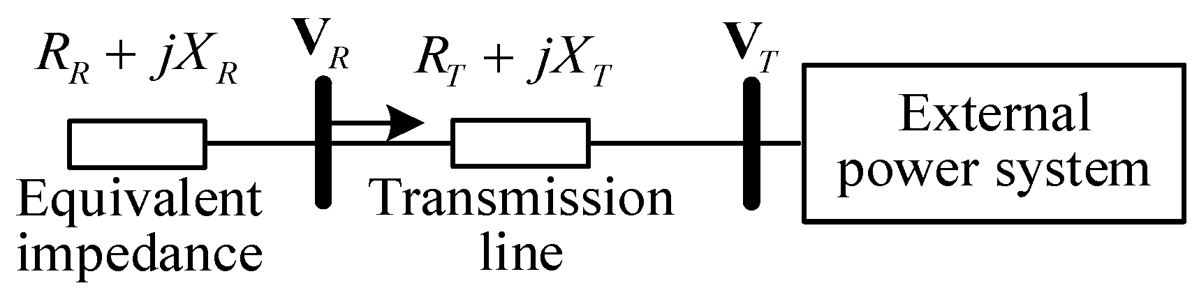
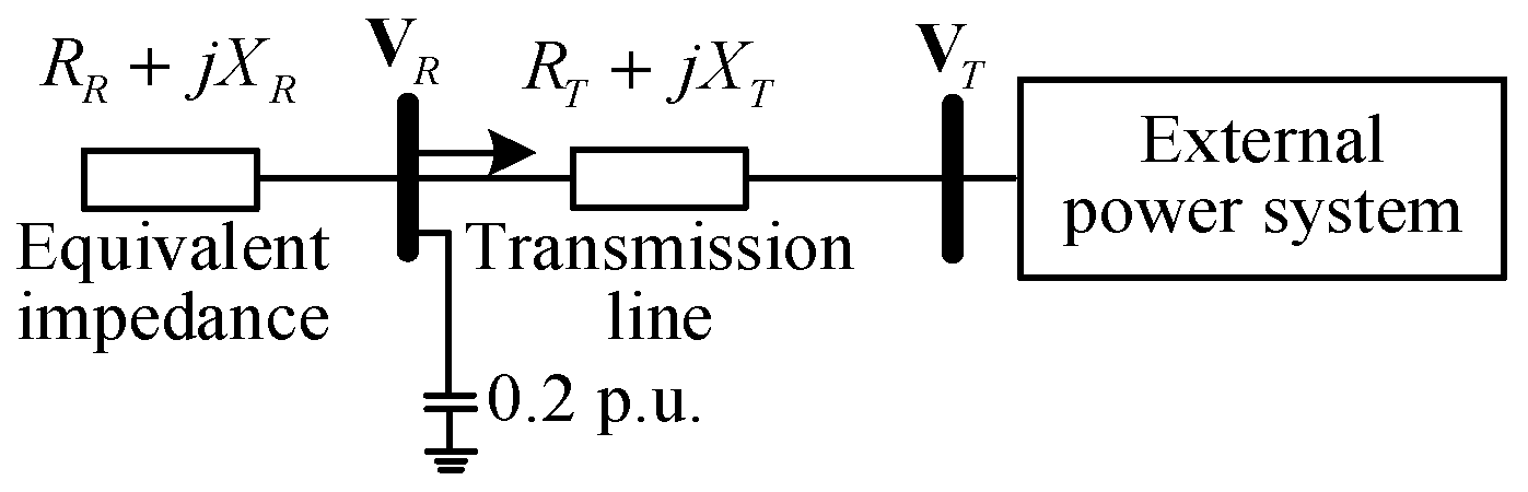
3.1. Review of Impedance Model Index

As depicted in Figure 1, it illustrates a distribution power system with single grid-connected renewable energy, referred to as a renewable energy single-infeed distribution power system, where $Z_T=R_T+j{X}_T$ represents the impedance of the transmission line, $P_R+j{Q}_R$ represents the output power of the grid-connected renewable energy, and $V_R$ represents the voltage vector at the renewable energy integration node, characterized by its amplitude $V_R$ and phase angle ${\theta }_R$. $V_T$ represents the voltage vector of the external system, with an amplitude $V_T$ and a phase angle of 0.

From Figure 1, it can be observed that there exists the following relationship between the voltage and power at the renewable energy-integration node:

$$V_T=V_R-(R_T+j{X}_T)\frac{P_R+j{Q}_R}{V_R}$$

(1)

Based on Equation (1), the following derivations can be obtained:

$$\left\{\begin{array}{l}{P}_R-\frac{V_R^2{R}_T}{R_T^2+X_T^2}=\frac{V_R{V}_T(X_T\sin {\theta }_R-R_T\cos {\theta }_R)}{R_T^2+X_T^2}\\ Q_R-\frac{V_R^2{X}_T}{R_T^2+X_T^2}=\frac{-V_R{V}_T(R_T\sin {\theta }_R+X_T\cos {\theta }_R)}{R_T^2+X_T^2}\end{array}\right.$$

(2)

By summing the squares on both sides of the above equations we yield

$${\left(P_R-\frac{V_R^2{R}_T}{R_T^2+X_T^2}\right)}^2+{\left(Q_R-\frac{V_R^2{X}_T}{R_T^2+X_T^2}\right)}^2=\frac{V_R^2{V}_T^2}{R_T^2+X_T^2}$$

(3)

Solving the Equation (3) with $V_R^2$ as a variable, it can be obtained that

$$V_R=\sqrt{P_R{R}_T+Q_R{X}_T+\frac{V_T^2}{2}\pm \sqrt{{\left(P_R{R}_T+Q_R{X}_T+\frac{V_T^2}{2}\right)}^2-Z_T^2\left(P_R^2+Q_R^2\right)}}$$

(4)

Based on the voltage and power at the renewable energy-integration node, the renewable energy can be equivalently represented at the node with an impedance:

$$Z_R=R_R+j{X}_R=\frac{V_R^2}{-P_R+j{Q}_R}$$

(5)

Equation (5) leads to the equivalent system of Figure 1, as illustrated in Figure 2.

Based on Figure 2, the impedance model index for the renewable energy single-infeed distribution power system can be formulated as

$$K_R=\frac{\left|Z_R\right|}{\left|Z_T\right|}=\frac{V_R^2}{\left|Z_T\right|\sqrt{P_R^2+Q_R^2}}$$

(6)

where | | represents the amplitude of a vector. According to Equation (6) when $K_R>1$, the system attains static-voltage stability; when $K_R=1$, the system achieves critical static-voltage stability; and when $K_R<1$, the system undergoes static-voltage instability [8].

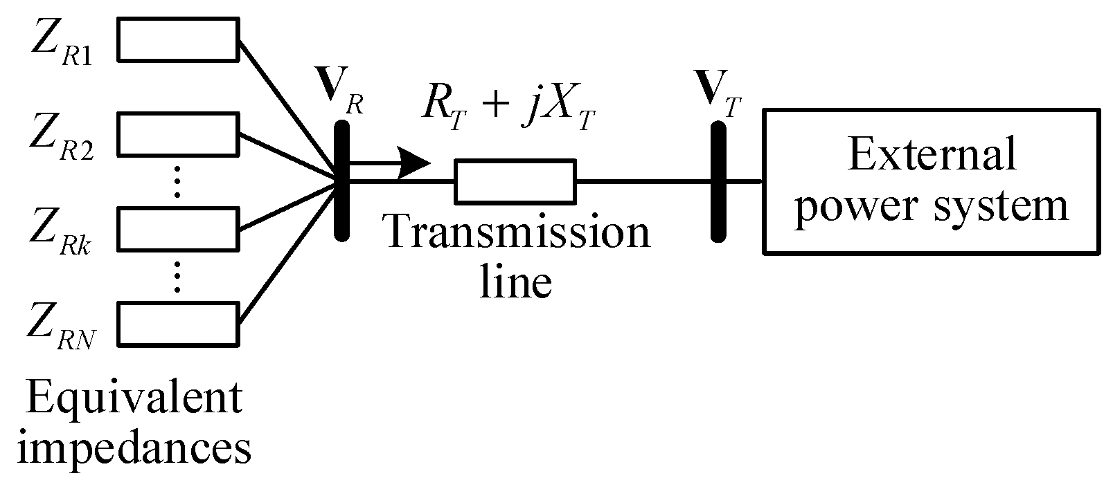
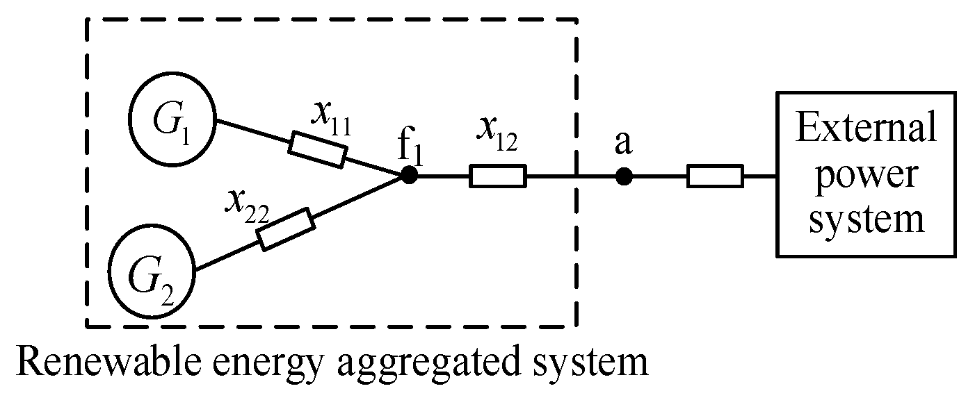
3.2. Simple Application of Impedance Model Index for Renewable Energy Aggregated Distribution Power Systems

As illustrated in Figure 3, it depicts an aggregated distribution power system comprising N renewable energy sources. In this configuration, N renewable energy sources are connected in parallel to a common node, where the equivalent impedance of the k^th renewable energy source is denoted as $Z_{Rk}$, k = 1, 2, 3,… N.

From Figure 3, the total equivalent impedance of the N renewable energy sources is

$$\left|Z_{Rs}\right|=\left|Z_{R1}//\cdots Z_{Rk}//\cdots //Z_{RN}\right|,$$

(7)

where // denotes a parallel connection between impedances.

Consequently, when considering N renewable energy sources as a collective entity for calculating the impedance model index of the system, its value is

$$K_{R1}=\frac{\left|Z_{Rs}\right|}{\left|Z_T\right|}$$

(8)

Equation (8) illustrates that when a single renewable energy source experiences static-voltage instability, multiple renewable energy sources aggregated systems will inevitably face static-voltage instability, but the reverse is not true. Consequently, static-voltage instability in renewable energy aggregated system invariably initiates at the main bus of the aggregated renewable energy sources. Therefore, the impedance model index for a renewable energy aggregated system should be computed based on the main bus of the aggregated renewable energy sources.

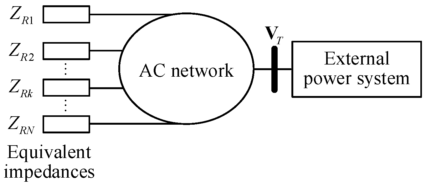
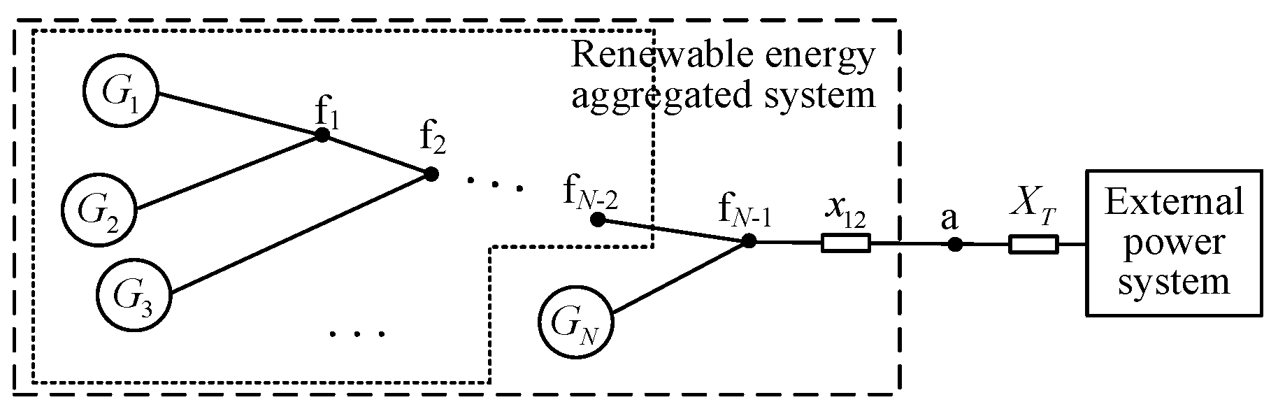
3.3. Proposed Static-Voltage-Stability Analysis Method Based on Impedance Model Index

Figure 4 represents a multi-infeed system with N renewable energy sources, where N renewable energy sources are connected to various nodes of the AC grid. The admittance matrix of the AC grid is $Y_N$; the equivalent impedance of N renewable energy sources is $Z_{eq}=\left[\begin{array}{cccccc}{Z}_{R1}& & & & & \\ & \ddots & & & & \\ & & Z_{Rk-1}& & & \\ & & & Z_{Rk}& & \\ & & & & \ddots & \\ & & & & & Z_{RN}\end{array}\right]$.

From $Y_N$ and $Z_{eq}$, the equation of the power system in Figure 4 is obtained as

$$Z_{eq}-{Y_N}^{-1}=0$$

(9)

By multiplying a matrix P and P⁻¹ to both sides of the Equation (9), respectively, it produces

$$P{Z}_{eq}{P}^{-1}-P{Y_N}^{-1}{P}^{-1}=Z_{eq}-\left[\begin{array}{ccc}{\rho }_1& & \\ & \ddots & \\ & & {\rho }_N\end{array}\right]=0$$

(10)

where ${\rho }_k$, k = 1,2,…,N is the k^th eigenvalue of the matrix ${Y_N}^{-1}$; P is the eigenvector matrix.

Therefore, the static-voltage stability can be determined using the N decoupled single-infeed distribution power system, where each system is composed of two series impedances, $Z_{Rk}$ and ${\rho }_k$.

We denote the maximum value of ${\rho }_k$ as ${\rho }_{\max }$; the static-voltage stability holds when

$$K_{Rk}=\frac{\left|Z_{Rk}\right|}{\left|{\rho }_{\max }\right|}>1$$

(11)

Comparing the proposed method to existing approaches for static-voltage stability analysis, this study offers the convenience of its application to large-scale renewable energy-connected power systems. Results can be obtained promptly, and the maximum dimension involved in calculations does not exceed the node number. Consequently, it addresses the time-consuming nature of traditional methods in dealing with complex power systems; details are listed in

Table 2. Compared results between the proposed method and the others.

Methods	The Method Proposed in This Paper
Continuation Power Flow Method in [24]	By calculating the impedance model index, static-voltage stability can be determined in a single computation, with the maximum dimension in calculations being equivalent to the node number. In contrast, the Continuation Power Flow Method requires multiple calculations of the voltage at each node, leading to time inefficiencies, particularly for large-scale power systems.
Impedance model index method in [8]	The impedance model index introduced in this paper facilitates the selection of network topology based on the impedance matrix of the network. Conversely, the impedance model index proposed in [8] necessitates the calculation of results for all nodes to make decisions about network selection, resulting in a time-consuming process.

.

3.4. Impact of Parameter Errors on Calculated Results of Static-Voltage Stability

From Equation (11), it can be known that parameter errors affect the results through two aspects: the first is Z_Rk, and the other is ρ_max. We denote the error as Δµ, the impact of which is calculated to be

$$\begin{array}{l}\Delta K_{Rk}=\frac{\left|Z_{Rk}\right|+\Delta \mu }{\left|{\rho }_{\max }\right|}-\frac{\left|Z_{Rk}\right|}{\left|{\rho }_{\max }\right|}=\frac{\Delta \mu }{\left|{\rho }_{\max }\right|}\\ \Delta K_{Rk}=\frac{\left|Z_{Rk}\right|}{\left|{\rho }_{\max }\right|+\Delta \mu }-\frac{\left|Z_{Rk}\right|}{\left|{\rho }_{\max }\right|}=-\frac{\left|Z_{Rk}\right|}{{\left|{\rho }_{\max }\right|}^2}\Delta \mu \end{array}$$

(12)

It can be seen from (12) that the impact of errors in different parts on the results is different. If the error occurs in Z_Rk, the deviation direction of the results is the same as that of the error; however, if it occurs in ρ_max, the deviation direction of the results is opposite to that of the error.

4. Analysis of Factors Affecting Static-Voltage Stability

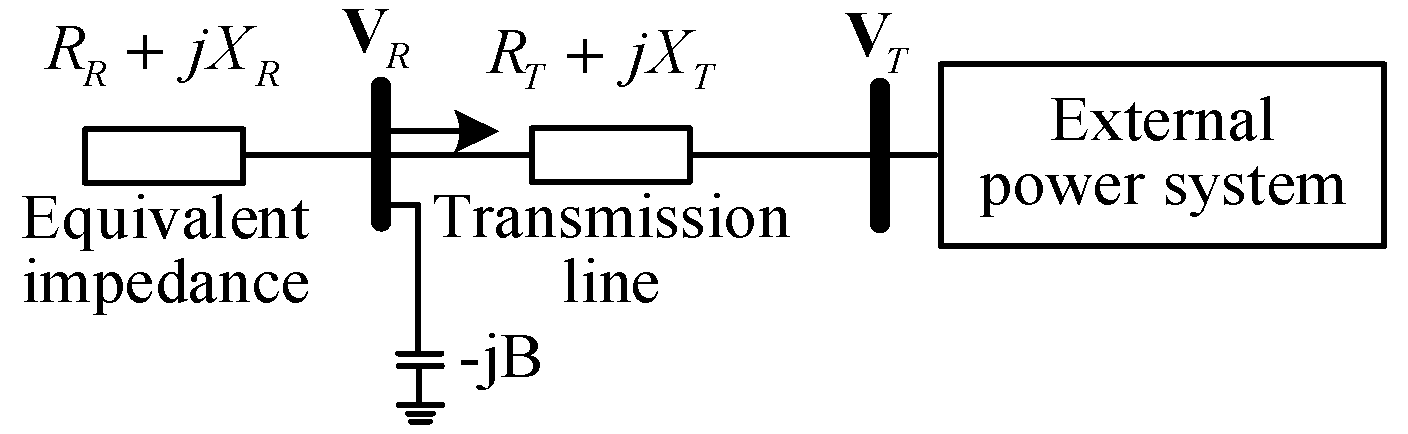
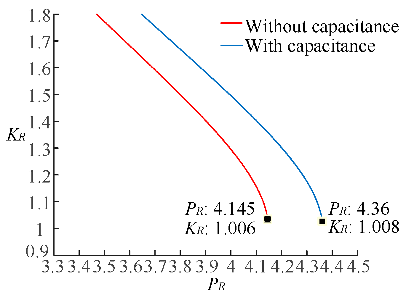
4.1. Impact of Reactive Power Compensation on Impedance Model Index

As illustrated in Figure 5, a shunt compensating capacitor is introduced at the renewable energy source integration node, with a capacitance value of B. The incorporation of the shunt capacitor alters the equivalent impedance of the transmission line from $Z_T$ to $Z_{Ts}$.

$$Z_{Ts}=\frac{1}{\frac{1}{R_T+j{X}_T}+\frac{1}{-jB}}=\frac{1}{\frac{1}{Z_T}+j\frac{1}{B}}$$

(13)

The parallel connection reduces the equivalent impedance of the transmission line, i.e., $\left|Z_{Ts}\right|<\left|Z_T\right|$. Consequently, the impedance model index at the renewable energy source integration node will increase, which is

$$K_R=\frac{\left|Z_R\right|}{\left|Z_{Ts}\right|}>\frac{\left|Z_R\right|}{\left|Z_T\right|}$$

(14)

From Equation (14), it is evident that increasing the reactive power compensation enhances the impedance model index at the renewable energy source integration node, thereby enhancing the static-voltage stability of the system.

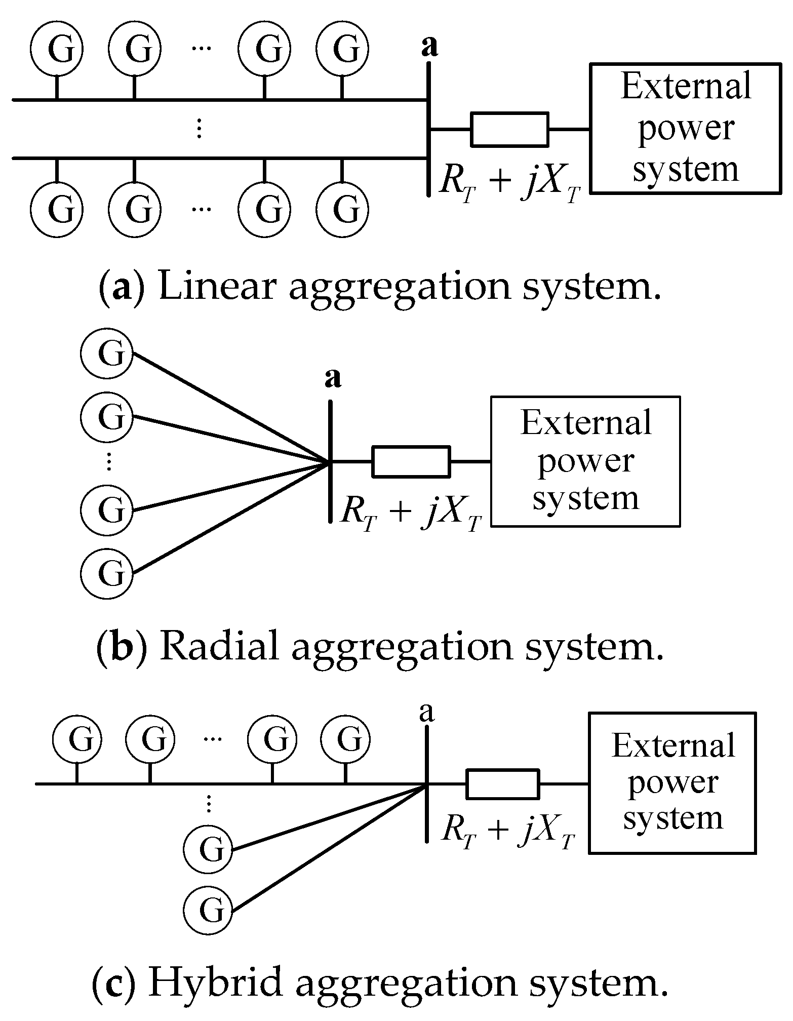
4.2. Influence of Renewable Energy Aggregation Topology on Static-Voltage Stability

Figure 6 presents various typical topologies of renewable energy aggregated distribution power systems, including linear, radial, and hybrid configurations. These three network topologies can be collectively represented using the generalized network structure shown in Figure 7.

In Figure 7, the impedance matrix of the generalized network topology can be expressed as

$$Z_N=X\otimes E_1,$$

(15)

where $\otimes$ represents the Kronecker product; $E_1=\left[\begin{array}{cc}k& -1\\ 1& k\end{array}\right]$; k is the ratio of unit resistance to unit reactance; and $X$ denotes the reactance matrix of the renewable energy aggregated system, which can be expressed as

$$X=\left[\begin{array}{cccc}{x}_{11}+X_T& x_{12}+X_T& \cdots & x_{1N}+X_T\\ x_{21}+X_T& x_{22}+X_T& \cdots & x_{2N}+X_T\\ ⋮& ⋮& \ddots & ⋮\\ x_{N1}+X_T& x_{N2}+X_T& \cdots & x_{NN}+X_T\end{array}\right],$$

(16)

where $x_{ij}$ represents the mutual reactance between the i^th and j^th renewable energy; $X_T$ signifies the equivalent reactance of the outgoing transmission lines of the renewable energy aggregated system.

$Y_N={Z_N}^{-1}$ is the admittance matrix of the system; evidently, the eigenvalues of $Y_N$ and $Z_N$ are reciprocals of each other. The larger the minimum eigenvalue of matrix $Y_N$, the greater the static-voltage-stability margin of the system. In other words, the smaller the maximum eigenvalue of $Z_N$ or $X$, the better the static-voltage stability of the system. Assuming the maximum eigenvalue of the matrix $X$ is ${\rho }_{\max }$, then

$${\rho }_{\max }=\max \left(P^{-1}XP\right),$$

(17)

where $P^{-1}$ and $P$ represent the left and right eigenvector matrices of matrix $X$. To ensure the best static-voltage stability of the system, the choice of aggregation system topology should favor the network topology with the smallest numerical value of ${\rho }_{\max }$. Next, we will delve into the analysis of the network topology with the smallest numerical value of ${\rho }_{\max }$ under identical line parameters.

As depicted in Figure 8, the system incorporates two renewable energy devices connected to node a through the AC network.

$$\begin{array}{l}{Z}_N=X\otimes E_1\\ X=\left[\begin{array}{cc}{x}_{11}+x_{12}+X_T& x_{12}+X_T\\ x_{12}+X_T& x_{22}+x_{12}+X_T\end{array}\right]\end{array}$$

(18)

From Equation (18), it is evident that when ${\rho }_{\max }$ takes its minimum value, there exists $x_{12}=0$, at which point node f1 and node a coincide. Therefore, when two renewable energy sources are directly connected in parallel to the aggregation bus node a, the system exhibits the best static-voltage stability.

Based on Equation (18), considering the general case of N renewable energy sources, as shown in Figure 9. Using induction, assume that (N − 1) renewable energy sources have already aggregated through (N − 2) internal nodes to node f_N−2, at which point the network topology formed by these (N − 1) renewable energy sources exhibits the best static-voltage stability, as depicted using the dashed box in Figure 9. To ensure the best static-voltage stability of the system in this scenario, the maximum eigenvalue of the network topology formed by node f_N−2 and the last renewable energy source should be minimized. Consequently, node f_N−1 coincides with node a. Therefore, when all renewable energy sources in the aggregation system are connected in parallel to the aggregation bus, the static-voltage stability of the renewable energy aggregated system is optimal. In other words, the radial aggregation system, as shown in Figure 6b, is the network topology with the best static-voltage stability.

5. Case Study Analysis

5.1. Impact of Reactive Power Compensation on Static-Voltage Stability

Figure 10 illustrates a single-infeed renewable energy system with a transmission line impedance of Z_T = 0.012 + j0.132 and a shunt capacitor at the integration point with a reactive compensation capacity of 0.2 p.u. The analysis is conducted by increasing the integration capacity of the renewable energy under two conditions: without capacitor compensation and with capacitor compensation. The voltage stability at the integration point is evaluated using the continuous power flow method, and the results are shown in Figure 11.

Figure 11 displays the P-V curve [27] at the integration point for the cases with and without capacitor compensation. The analysis reveals that the integration capacity of the renewable energy source is approximately 4.15 p.u. without capacitor compensation, beyond which the system experiences static-voltage instability. With capacitor compensation, the integration capacity of the renewable energy source is approximately 4.36 p.u., and exceeding this value also leads to static-voltage instability. These results demonstrate that increasing reactive compensation enhances the integration capacity of the renewable energy source. In this scenario, the impedance model index at the integration point for different integration capacities is calculated and shown in Figure 12.

Figure 12 illustrates the variation of the impedance model index at the integration point with increasing integration capacity. When the integration capacity of renewable energy reaches its limit, the system exhibits critical static-voltage instability. At this point, the impedance model index is approximately 1.006 without capacitor compensation and approximately 1.008 with capacitor compensation. From Figure 11 and Figure 12, it can be observed that as the renewable energy-integration capacity gradually increases and approaches the static-voltage-stability limit, the impedance model index decreases continuously and converges towards 1. The presence of reactive compensation in the renewable energy-integration system results in a higher impedance model index compared to the case without compensation. This conclusion is consistent with the analysis results from the P-V curve, which confirms that the impedance model index accurately reflects the static-voltage stability of the system.

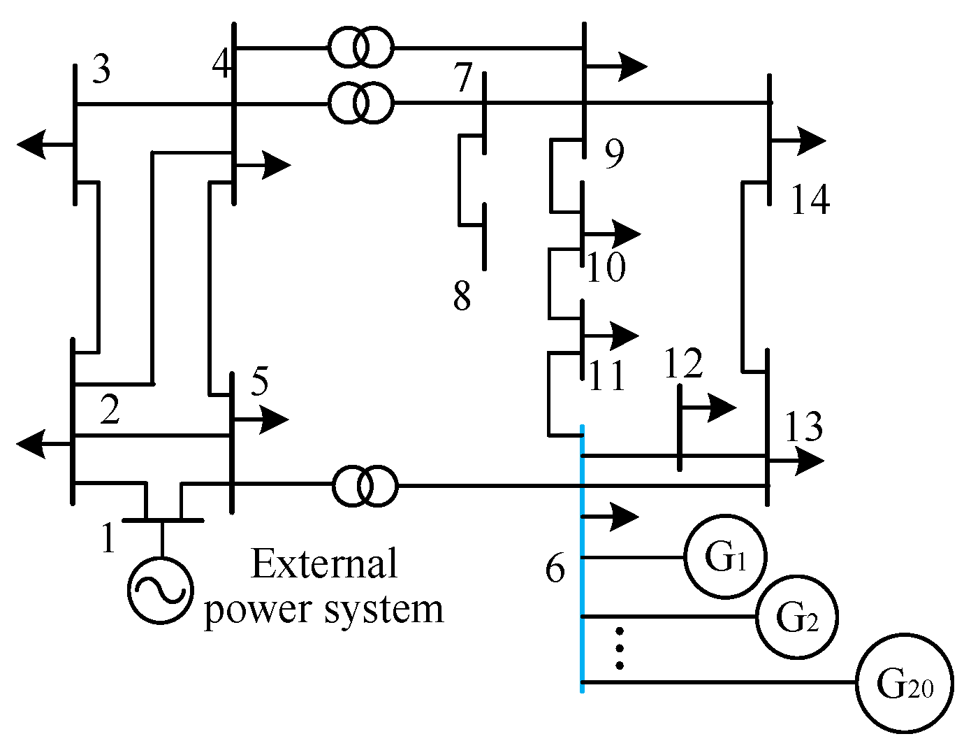
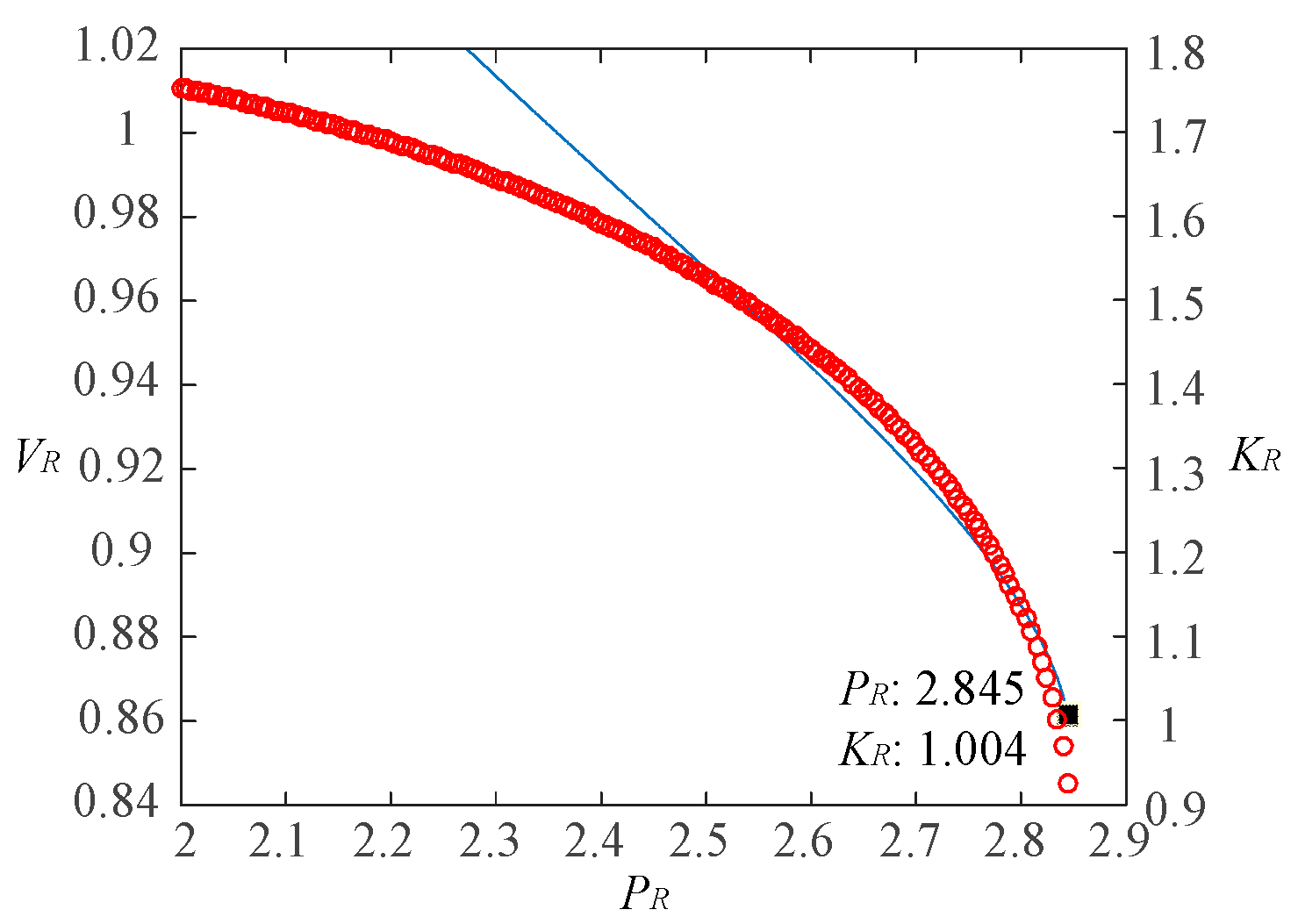
5.2. Calculation of Impedance Model Index for Renewable Energy Aggregated Distribution Power Systems

Figure 13 represents a renewable energy aggregated system with 20 renewable energy sources. The system parameters are based on the IEEE 14-bus system, with modifications as follows: the network loads are changed from constant power loads to constant impedance loads, the generators except for node 1 are removed, and 20 renewable energy units are paralleled at node 6. The impedance between each renewable energy unit and the aggregation bus is 0.0002 + j0.03 p.u., while other parameters remain the same as in the original IEEE 14-bus system.

Figure 14 illustrates the P-V curve and impedance model index variation at node 6 (aggregation bus) as the total capacity of the renewable energy units increases. The results are obtained by first calculating the equivalent impedance of the renewable energy units and then using the continuous power flow method to calculate the voltage amplitude at node 6 for increasing power capacities.

The analysis indicates that as the total capacity of the renewable energy units increases; the impedance model index decreases and approaches 1, suggesting that the static-voltage stability of the system gradually deteriorates. When the total integration capacity of the renewable energy units reaches 2.85 p.u., the impedance model index is approximately 1.004, indicating that the system is at the critical static-voltage-instability state. Beyond this value, the system experiences static-voltage instability. The analysis results from the P-V curve align with the above analysis, confirming the accuracy of the impedance model index calculation and the reliability of the analysis results.

To further verify that the differences in the integration capacities of individual renewable energy units do not affect the analysis results, the 20 renewable energy units are divided into three groups: 6, 6, and 7 units per group. Each group has different capacities, as shown in the first column of

Table 3. Calculation results of the impedance model index for the renewable energy aggregated system.

Capacities of Each Group of Renewable Energy Sources	Aggregation Bus Maximum Grid-Connected Capacity	$\mathbf{Impedance}\mathbf{Model}\mathbf{Index}{\mathit{K}}_{\mathit{R}}$
0.115, 0.145, 0.165	2.842	1.008
0.165, 0.130, 0.135	2.841	1.010
0.135, 0.150, 0.140	2.838	1.012

. The total integration capacity at the aggregation bus (node 6) is calculated for each group, as shown in the second column of Table 3. It is observed that the differences in renewable energy unit capacities have little impact on the total integration capacity at the aggregation bus, which remains at approximately 2.8 p.u. When the renewable energy-integration capacity reaches its limit, the system experiences static-voltage instability, and the impedance model index at the aggregation bus is approximately 1, regardless of the different capacities of the renewable energy units within the aggregation system.

From Table 3, it is evident that regardless of the differences in renewable energy unit capacities, the total integration capacity at the aggregation node remains nearly unchanged at approximately 2.8 p.u. At the critical state when the renewable energy-integration capacity reaches its limit, the impedance model index is approximately 1 at the aggregation node. Thus, the impedance model index calculation method proposed in this study effectively reflects the static-voltage-stability margin of the system. The impedance model index is not influenced by the different capacities of renewable energy units within the aggregation system but is only related to the total integration capacity at the aggregation node.

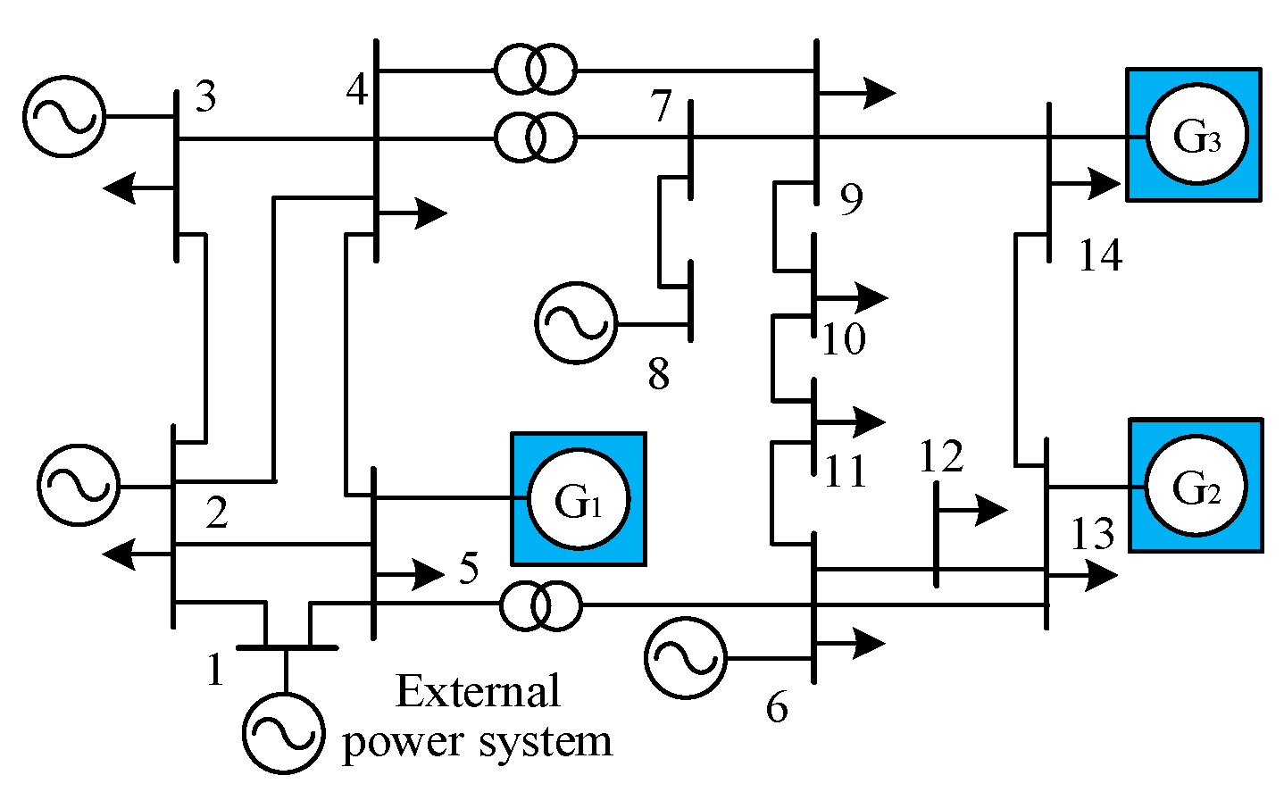
5.3. Calculation of Impedance Model Index for Renewable Energy Multi-Infeed Distribution Power Systems

Figure 15 depicts a multi-infeed distribution power system with three renewable energy units, G1, G2, and G3, connected to nodes 5, 13, and 14, respectively, in the IEEE 14-bus system. In this section, three case studies are performed to analyze the impact of each renewable energy unit’s maximum integration capacity on the system’s static-voltage stability, while ensuring the system remains stable.

Case 1: The integration capacities of renewable energy units G2 and G3 are fixed at 1 p.u., and the impact of renewable energy unit G1’s integration capacity on the system’s static-voltage stability is analyzed.

Figure 16 shows the P-V curve and the impedance model index variation at node 5 as the integration capacity of renewable energy unit G1 increases. The calculation starts by determining the equivalent impedances of renewable energy units G2 and G3, which are then used as self-admittances at nodes 13 and 14, respectively. Next, the equivalent impedance of the transmission line between node 5 and node 1 is computed. Finally, the impedance model index at node 5 is calculated for different integration capacities of renewable energy unit G1, as shown using the blue curve in Figure 16. Furthermore, the voltage amplitude at node 5 is calculated using the continuous power flow method as the power capacity of renewable energy unit G1 increases from 8 p.u. to 8.4 p.u., shown with the red curve in Figure 16.

From Figure 16, it is evident that as the integration capacity of the renewable energy unit G1 increases, the impedance model index decreases and approaches 1, indicating a gradual decline in the system’s static-voltage stability. When the total integration capacity of the renewable energy unit G1 at node 5 reaches 8.37 p.u., the impedance model index is approximately 1.038, signifying that the system is at a critical static-voltage instability state. Beyond this value, the system experiences static-voltage instability. The analysis results from the P-V curve are consistent with the above analysis, demonstrating the accuracy of the impedance model index calculation and the reliability of the analysis results.

Case 2: The integration capacities of renewable energy units G1 and G3 are fixed at 1 p.u., and the impact of renewable energy unit G2’s integration capacity on the system’s static-voltage stability is analyzed.

Figure 17 displays the P-V curve and the impedance model index variation at node 13 as the integration capacity of renewable energy unit G2 increases. The calculation process is similar to Case 1, with the equivalent impedances of renewable energy units G1 and G3 used as self-admittances at nodes 5 and 14, respectively. The equivalent impedance of the transmission line between node 13 and node 1 is computed, and then the impedance model index at node 13 is calculated for different integration capacities of renewable energy unit G2, as shown with the blue curve in Figure 17. The voltage amplitude at node 13 is determined using the continuous power flow method as the power capacity of renewable energy unit G2 increases from 2.2 p.u. to 2.45 p.u., shown using the red curve in Figure 17.

From Figure 17, it is observed that as the integration capacity of renewable energy unit G2 increases, the impedance model index decreases and approaches 1, indicating a decline in the system’s static-voltage stability. When the total integration capacity of renewable energy unit G2 at node 13 reaches 2.45 p.u., the impedance model index is approximately 1.064, signifying that the system is at the critical static-voltage-instability state. Beyond this value, the system experiences static-voltage instability. The analysis results from the P-V curve align with the above analysis, demonstrating the accuracy of the impedance model index calculation and the reliability of the analysis results.

Case 3: The integration capacities of renewable energy units G1 and G2 are fixed at 1 p.u., and the impact of renewable energy unit G3’s integration capacity on the system’s static-voltage stability is analyzed.

Figure 18 shows the P-V curve and the impedance model index variation at node 14 as the integration capacity of renewable energy unit G3 increases. The calculation procedure is similar to Case 1 and Case 2. The equivalent impedances of renewable energy units G1 and G2 are used as self-admittances at nodes 5 and 13, respectively, and the equivalent impedance of the transmission line between node 14 and node 1 is computed. Then, the impedance model index at node 14 is calculated for different integration capacities of renewable energy unit G3, as shown with the blue curve in Figure 18. The voltage amplitude at node 14 is determined using the continuous power flow method as the power capacity of renewable energy unit G3 increases from 2.0 p.u. to 2.3 p.u., shown using the red curve in Figure 18.

From Figure 18, it is evident that as the integration capacity of the renewable energy unit G3 increases, the impedance model index decreases and approaches 1, indicating a decline in the system’s static-voltage stability. When the total integration capacity of the renewable energy unit G3 at node 14 reaches 2.26 p.u., the impedance model index is approximately 1.01, signifying that the system is at the critical static-voltage-instability state. Beyond this value, the system experiences static-voltage instability. The analysis results from the P-V curve are consistent with the above analysis, demonstrating the accuracy of the impedance model index calculation and the reliability of the analysis results.

Based on the above calculation results, it is evident that the impedance model index is also applicable to the renewable energy multi-infeed system. For different integration nodes in the system, the maximum integration capacity of renewable energy units varies, and each node’s integration capacity limit can be evaluated using the corresponding limit power at which the impedance model index equals 1. If the integration capacities of renewable energy units are the same, selecting the node with the highest impedance model index as the integration node will result in the best static-voltage stability for the system.

5.4. Impact of Network Topology on Impedance Model Index

Figure 19 illustrates a multi-infeed distribution power system with four renewable energy units, G1, G2, G3, and G4, connected to nodes 11, 12, 13, and 14, respectively, in the IEEE 14-bus system. Each renewable energy unit outputs power at 0.5 p.u. Additionally, an AC branch with an impedance of 0.05 + j0.12 is added between node 1 and node 11, as shown using the green line in the figure. The impedance model index calculation results for nodes 11, 12, 13, and 14 are presented in

Table 4. Impedance model index as affected by adding AC branch.

	${\mathit{K}}_{\mathit{R}1}$	${\mathit{K}}_{\mathit{R}2}$	${\mathit{K}}_{\mathit{R}3}$	${\mathit{K}}_{\mathit{R}4}$
Before Adding AC Branches	1.5412	1.3155	1.4870	1.2717
After Adding AC Branches	5.0474	1.6547	2.1329	1.6498
Improvement Margin of the Index (%)	227.50	25.78	43.44	29.73

.

Table 4 demonstrates that adding the AC branch increases the impedance model index at each integration node, indicating that adding AC lines can enhance the system’s static-voltage stability. The impedance model index at node 11 experiences a significant increase, suggesting that node 11 can accommodate more renewable energy units after the AC line is connected.

Similarly, a DC line is added between node 1 and node 14 in the system, with constant power control, transmitting power at 0.3 p.u. Node 14 serves as the infeed end of the DC line, and node 1 serves as the outfeed end, as shown with the blue line in Figure 20. The impedance model index calculation results for nodes 11, 12, 13, and 14 are shown in

Table 5. Impedance model index as affected by adding DC branch.

	${\mathit{K}}_{\mathit{R}1}$	${\mathit{K}}_{\mathit{R}2}$	${\mathit{K}}_{\mathit{R}3}$	${\mathit{K}}_{\mathit{R}4}$
Before DC Line Connection	1.5412	1.3155	1.4870	1.2717
After DC Line Connection	1.5462	1.3351	1.5062	1.3297
Improvement Margin of the Index (%)	0.32	1.49	1.29	4.56

.

Table 5 shows that after adding the DC transmission line, the impedance model index at each integration node increases, indicating that adding DC transmission lines can improve the system’s static-voltage stability. The impedance model index at node 14 experiences the most significant increase, suggesting that node 14 can accommodate more renewable energy units after the DC transmission line is connected.

Based on the analysis results of these two case studies, it is evident that increasing AC or DC transmission lines can alter the original topology of the transmission network, thereby enhancing the static-voltage stability of the renewable energy-integration system.

6. Conclusions

In this study, an equivalent impedance model for renewable energy-integrated distribution power systems was established. Based on the saddle-node bifurcation theory of static-voltage stability, an impedance model index applicable to generalized renewable energy-integrated distribution power systems was proposed, and the criterion for static-voltage stability of the system based on the impedance model index was derived. Using the proposed analysis method, the impact of the number, location, and network topology of renewable energy integration on the system’s static-voltage stability was analyzed, providing valuable insights for selecting suitable locations for renewable energy integration and planning renewable energy-integration capacities. The specific conclusions are as follows:

• The impedance model index proposed in this study is not only applicable to renewable energy single-infeed distribution power systems but also suitable for renewable energy multi-infeed distribution power systems. It effectively reflects the static-voltage-stability margin of the renewable energy-integration nodes.
• The network topology of renewable energy aggregated systems can affect the static-voltage stability of the distribution power system. This study demonstrated that the radiation-type network topology for renewable energy offers the best static-voltage stability of the distribution power system.
• The addition of AC and DC lines can increase the impedance model index, thereby improving the system’s static-voltage stability. When planning the integration of renewable energy, selecting the node with the highest impedance model index can enhance the stability of the distribution power system.
• This study offers valuable insights into the static-voltage stability of renewable energy-integrated distribution power systems, and considering the fast development of EVs, this proposed method also has huge application scope in the future in similar scenarios, enhancing decision-making in renewable energy planning and operation. Future studies will consider the intermittency of active power generation.

References

1. Tielens, P.; Van Hertem, D. The relevance of inertia in power systems. New Sustain. Energy Rev. 2016, 55, 999–1009. [Google Scholar] [CrossRef]
2. Kundur, P.; Paserba, J.; Ajjarapu, V.; Andersson, G.; Bose, A.; Canizares, C.; Hatziargyriou, N.; Hill, D.; Stankovic, A.; Taylor, C.; et al. Definition and classification of power system stability. IEEE Trans. Power Syst. 2004, 19, 1387–1401. [Google Scholar]
3. Hatziargyriou, N.; Milanovic, J.; Rahmann, C.; Ajjarapu, V.; Canizares, C.; Erlich, I.; Hill, D.; Hiskens, I.; Kamwa, I.; Pal, B.; et al. Definition and classification of power system stability–Revisited & extended. IEEE Trans. Power Syst. 2021, 36, 3271–3281. [Google Scholar]
4. Xie, X.; He, J.; Mao, H.; Li, H. New Issues and Classification of Power System Stability with High Shares of News and Power Electronics. Proc. CSEE 2021, 41, 461–473. [Google Scholar]
5. Ge, P.; Xiao, F.; Tu, C.; Guo, Q.; Gao, J.; Song, Y. Comprehensive transient stability enhancement control of a VSG considering power angle stability and fault current limitation. CSEE J. Power Energy Syst. 2022, 1–10. [Google Scholar] [CrossRef]
6. Laiva Roca, D.A.; Mercado, P.; Suvire, G. System Frequency Response Model Considering the Influence of Power System Stabilizers. IEEE Lat. Am. Trans. 2022, 20, 912–920. [Google Scholar] [CrossRef]
7. Ranjan, S.; Das, D.C.; Latif, A.; Sinha, N.; Hussain, S.M.S.; Ustun, T.S. Maiden Voltage Control Analysis of Hybrid Power System with Dynamic Voltage Restorer. IEEE Access 2021, 9, 60531–60542. [Google Scholar] [CrossRef]
8. Song, Y.; Hill, D.J.; Liu, T. Static Voltage Stability Analysis of Distribution Systems Based on Network-Load Admittance Ratio. IEEE Trans. Power Syst. 2019, 34, 2270–2280. [Google Scholar] [CrossRef]
9. US-Canada Power Outage Task Force. Final Report on the August 14th 2003 Blackout in the United States and Canada. Available online: http://www.ferc.gov/ (accessed on 1 October 2023).
10. Australian Energy Market Operator. Black System South Australia 28 September 2016–Third Preliminary Report; Australian Energy Market Operator Limited: Melbourne, Australia, 2016. [Google Scholar]
11. Xue, Y.; Xu, T.; Liu, B.; Li, Y. Quantitative assessments for transient voltage security. IEEE Trans. Power Syst. 2000, 15, 1077–1083. [Google Scholar] [CrossRef]
12. Ellithy, K.; Shaheen, M.; Al-Athba, M.; Al-Subaie, A.; Al-Mohannadi, S.; Al-Okkah, S.; Abu-Eidah, S. Voltage stability evaluation of real power transmission system using singular value decomposition technique. In Proceedings of the IEEE 2nd International Power and Energy Conference, Johor Bahru, Malaysia, 1–3 December 2008; pp. 1691–1695. [Google Scholar] [CrossRef]
13. Alzaareer, K.; Saad, M.; Mehrjerdi, H.; Salem, Q.; Harasis, S.; Aldaoudeyeh, A.-M.I.; Al-Masri, H.M.K. Sensitivity Analysis for Voltage Stability Considering Voltage Dependent Characteristics of Loads and DGs. IEEE Access 2021, 9, 156437–156450. [Google Scholar] [CrossRef]
14. Nirbhavane, P.S.; Corson, L.; Rizvi, S.M.H.; Srivastava, A.K. TPCPF: Three-Phase Continuation Power Flow Tool for Voltage Stability Assessment of Distribution Networks with Distributed Energy Resources. IEEE Trans. Ind. Appl. 2021, 57, 5425–5436. [Google Scholar] [CrossRef]
15. Flueck, A.J.; Gonella, R.; Dondeti, J.R. A new power sensitivity method of ranking branch outage contingencies for voltage collapse. IEEE Trans. Power Syst. 2002, 17, 265–270. [Google Scholar] [CrossRef]
16. Pierrou, G.; Wang, X. Analytical Study of the Impacts of Stochastic Load Fluctuation on the Dynamic Voltage Stability Margin Using Bifurcation Theory. IEEE Trans. Circuits Syst. I Regul. Pap. 2020, 67, 1286–1295. [Google Scholar] [CrossRef]
17. Lim, J.M.; DeMarco, C.L. SVD-Based Voltage Stability Assessment from Phasor Measurement Unit Data. IEEE Trans. Power Syst. 2016, 31, 2557–2565. [Google Scholar] [CrossRef]
18. Gao, B.; Morison, G.K.; Kundur, P. Voltage stability evaluation using modal analysis. IEEE Trans. Power Syst. 1992, 7, 1529–1542. [Google Scholar] [CrossRef]
19. Pan, X.; Li, L.; Huang, H.; Yan, J.; Yang, L. Method for evaluating voltage weak area of AC power system at DC receiving end considering sensitivity and static voltage stability margin. Electr. Power Autom. Equip. 2019, 39, 1–8. [Google Scholar]
20. Cui, X.; Yun, Z.; Liu, D.; Yang, H.; Li, Z.; Gao, D.; Jin, X. A New Method of Sensitivity Analysis for Static Voltage Stability Online Prevention and Control of Large Power Grids. Power Syst. Technol. 2020, 44, 246–254. [Google Scholar]
21. Zhou, J.; He, Y.; He, H.; Li, C.; Li, P. Calculation Method for Continuation Power Flow Based on Line Voltage Stability Index. Proc. CSU EPSA 2018, 30, 140–144. [Google Scholar]
22. Chen, G.; Zhou, Y.; Zhao, J.; Huang, G.; Bao, Y.; Lin, Q. A Three-Stage Progressive Voltage Stability Contingency Screening and Ranking Method for Large Power Grids. South. Power Syst. Technol. 2018, 12, 70–75. [Google Scholar]
23. Chen, C.; Jiang, T.; Wan, K.; Feng, Z. Improved point of collapse method for direct calculation of static voltage stability margin. Electr. Power Autom. Equip. 2020, 40, 150–155. [Google Scholar]
24. Tang, X.; Gao, L. Analysis on Static Voltage Stability Considering Restriction of Branch Power. Power Syst. Technol. 2011, 35, 99–102. [Google Scholar]
25. Kwatny, H.G. Static bifurcati on in electric power networks: Loss of steady-state stability and voltage collapse. IEEE Trans CAS 1986, 33, 981–991. [Google Scholar] [CrossRef]
26. Chiang, H.D.; Ju Meau, R.J. A more efficient formulation for computation of the maximum loading in electric power system. IEEE Trans Power Syst. 1995, 10, 635–646. [Google Scholar] [CrossRef]
27. Kamaruzzaman, Z.A.; Mohamed, A. Impact of grid-connected photovoltaic generator using P-V curve and improved voltage stability index. In Proceedings of the IEEE International Conference on Power and Energy (PECon), Kuching, Malaysia, 1–3 December 2014; pp. 196–200. [Google Scholar]
Figure 1. Schematic diagram of a renewable energy single-infeed distribution power system.
Energies 17 01028 g001
Figure 2. Schematic diagram of the equivalent structure of a renewable energy single-infeed distribution power system.
Energies 17 01028 g002
Figure 3. A renewable energy aggregated distribution power system.
Energies 17 01028 g003
Figure 4. Multi-infeed distribution power system with N renewable energy sources.
Energies 17 01028 g004
Figure 5. Schematic diagram of a renewable energy-integrated system with reactive power compensation.
Energies 17 01028 g005
Figure 6. Typical network topology of a renewable energy aggregated distribution power systems. “a” is the connection point of renewable energy clusters to the external power system.
Energies 17 01028 g006
Figure 7. Generalized network topology of renewable energy aggregated distribution power systems. “a” is the connection point of renewable energy clusters to the external power system.
Energies 17 01028 g007
Figure 8. Structure of distribution power system with two renewable energy sources. “a” is the connection point of renewable energy clusters to the external power system. Point f1 marks the intersection of the internal networks of the two renewable energy sources. x11, x22, respectively, represent the reactance between renewable energy sources G1, G2, and a node f1. x12 represents the reactance between points a and f1.
Energies 17 01028 g008
Figure 9. Structure of distribution power system with N renewable energy sources. Gk, represents the kth renewable energy, k = 1, 2, …, N, fj, j = 1, 2, …, N − 1, represents the jth intersection point of the internal networks.
Energies 17 01028 g009
Figure 10. Schematic diagram of a single-infeed renewable energy system with reactive power compensation.
Energies 17 01028 g010
Figure 11. P-V curve of the grid-connected node in a single-infeed renewable energy system.
Energies 17 01028 g011
Figure 12. Variation curve of the impedance model index in a single-infeed renewable energy system.
Energies 17 01028 g012
Figure 13. Schematic diagram of a distribution power system with 20 renewable energy sources. Blue line: collection node of 20 renewable energy units.
Energies 17 01028 g013
Figure 14. P-V curve and impedance model index variation curve at node 6. Red line: P-V curve. Blue line: impedance model index curve.
Energies 17 01028 g014
Figure 15. Schematic diagram of a multi-infeed distribution power system. G1, G2, and G3, represent three renewable energy units, respectively.
Energies 17 01028 g015
Figure 16. P-V curve and impedance model index variation curve at node 5. Red line: P-V curve. Blue line: impedance model index curve.
Energies 17 01028 g016
Figure 17. P-V curve and impedance model index variation curve at node 13. Red line: P-V curve. Blue line: impedance model index curve.
Energies 17 01028 g017
Figure 18. P-V curve and impedance model index variation curve at node 14. Red line: P-V curve. Blue line: impedance model index curve.
Energies 17 01028 g018
Figure 19. A renewable energy multi-infeed distribution power system with an additional AC branch. Green line: added AC branch. G1, G2, G3, and G4 represent four renewable energy units, respectively.
Energies 17 01028 g019
Figure 20. A renewable energy multi-infeed distribution power system with an additional DC branch. Green line: added DC branch. G1, G2, G3, and G4 represent four renewable energy units, respectively.
Energies 17 01028 g020