A Bi-Level Optimal Scheduling Strategy for Microgrids for Temperature-Controlled Capacity and Time-Shifted Capacity, Considering Customer Satisfaction

Abstract

Since microgrids can effectively integrate renewable energy, energy storage devices, and controllable loads, this advantage promotes the rapid development and application of microgrid technology. However, with the high proportion of renewable energy access, only considering how energy is optimally distributed in microgrids can no longer meet the actual demand. How to aggregate user-side controllable loads to form regulation resources has become a research hotspot, and the users, as a passive party in the load scheduling process, should also be an important consideration in their perception of the use of electricity. First, a control model for temperature-controlled loads and a time-shift model for time-shiftable loads are developed. Then, the comprehensive electricity satisfaction model of users is established, and the two-layer optimal scheduling model of microgrids considering users’ satisfaction is proposed, with users as the upper layer and microgrids as the lower layer, and the two-layer model is transformed into a single-layer model according to the KKT condition for solving. Finally, the effect of the weighting factor for satisfaction on the economy is discussed through the analysis of examples, which verifies the effectiveness of the two-layer model.

1. Introduction

Microgrids are an important part of smart grid development, which have received more and more attention due to their environmental friendliness and flexible operation modes. Many scholars have studied the energy distribution of microgrids; reference [1] proposes a two-tier robust capacity planning model for PV-Wind-Storage-Diesel, considering wind uncertainty and standby demand scenarios. Reference [2] proposes an optimization method for hybrid energy storage capacity allocation based on the role of energy storage devices in peak shaving and smoothing distributed generation. References [3,4,5,6] establish a model for the optimal allocation of the microgrid power supply from the perspective of reducing investment costs and improving power supply revenue. The above studies mainly focus on how energy can be optimally allocated to make the microgrid have the highest total benefits, but none of them consider the impact of load-side resources on the optimal economic operation of microgrids.

With the continuous development of information technology, the intelligence level of load control has also gradually improved. More refined operational information on loads can now be obtained through advanced computer technology [7]. In fact, there are a large number of dispatchable resources in the power system. Currently, there is more research on dispatchable loads. Reference [8] utilized the flexible dispatch characteristics of electric heating to consume the new energy output prediction deviation. Reference [9] established a temperature-controlled load aggregation model and evaluated the temperature-controlled load cluster responsiveness and distribution characteristics. Reference [10] established peak shaving and valley filling as the goal of the electric heat pump aggregation control model. Reference [11] utilized the electric heating cluster control strategy to achieve the goal of reducing coal consumption and consuming renewable energy. Although the above study realizes the aggregation of temperature-controlled loads, it does not consider the different response ability of temperature-controlled loads of users with different economic conditions and housing structures. Meanwhile, there are a large number of time-shiftable loads on the load side that are friendly and cooperative with the grid, in addition to temperature-controlled loads. Reference [12] proposes an energy optimization method that includes distributed power sources, energy storage, and time-shiftable loads. Reference [13] proposes a portfolio model that combines flexible loads, distributed power sources, and demand response to improve system returns. Reference [14] developed a power capacity optimization model, taking into account controllable loads. While the above study has investigated the characteristics of temperature-controlled and time-shiftable loads to meet the challenges of participating in renewable energy consumption, the process occurs due to the shifting of the load profile, which in turn affects the electricity consumption habits of the consumers. The above study did not consider the satisfaction bias caused by changing the electricity usage habits of the users. Therefore, there is a need to consider the customer’s satisfaction with electricity usage as a factor. The integrated consideration of microgrid benefits and user satisfaction reflects the emphasis on the dual needs of economic efficiency and user experience in the power system.

To synthesize the above problems, this paper first forms a direct load control (DLC) scheduling model with load aggregators (LA) for distributed single electric heating in different buildings. The thermal parameters of different types of dwellings are clustered, the user population is divided, and the corresponding comfort boundaries are individually designed for different populations. Then, the total temperature-controlled capacity of the electric heating is calculated by the alternate control strategy. Considering the case of electric heating, three kinds of commonly used time-shifted loads for residents are added and their electricity consumption characteristics are analyzed to establish a time-shifted capacity model. Deviation of the dispatched load profile from the original load profile is used as a measure of satisfaction. Finally, a bi-level optimization model for a microgrid with comprehensive satisfaction as the upper model and microgrid benefit function as the lower model is established; the impacts of temperature-controlled capacity and time-shifted capacity on new energy consumption, as well as the economics of scheduling results in different scenarios, are discussed through the analysis of arithmetic examples.

The innovations of this paper include (1) a temperature-controlled capacity model based on alternating control, as well as a time-shifted capacity model based on time margins; (2) a satisfaction model for each of the two types of residential dispatchable load users, resulting in a greater focus on the user experience while ensuring economic efficiency; and (3) a two-layer optimization model based on the KKT condition, with satisfaction as the upper layer and microgrid benefits as the lower layer.

The temperature-controlled capacity model and time-shifted capacity model are presented in Section 2, respectively; the microgrid system including distributed power sources, energy storage devices, and loads is introduced in Section 3; a two-tier optimal scheduling model for microgrids is presented in Section 4; simulation analyses are performed in Section 5 to quantify the economics of the microgrid system; and finally, this paper is summarized.

2. Temperature-Controlled Capacity and Time-Shifted Capacity Modeling

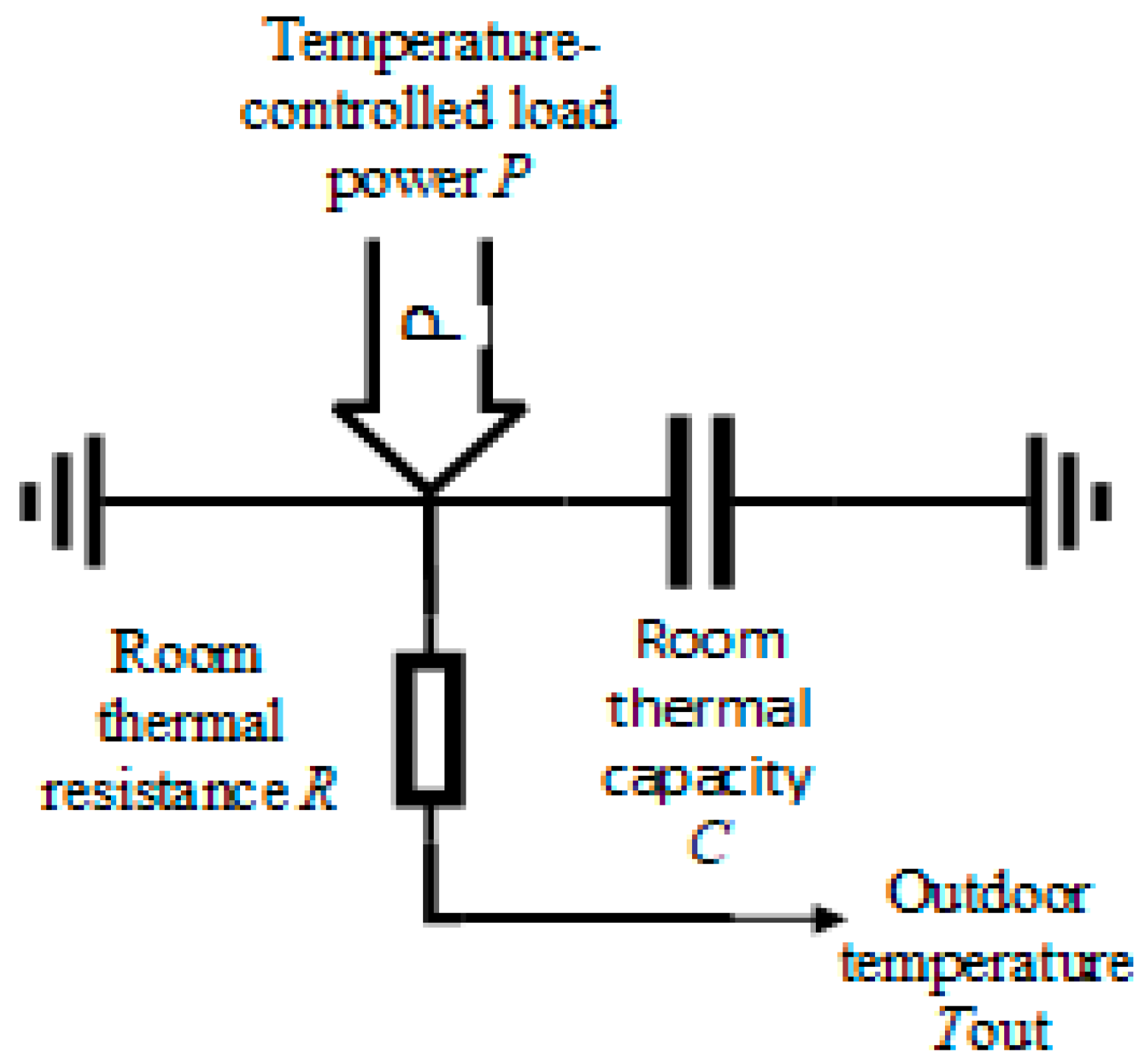
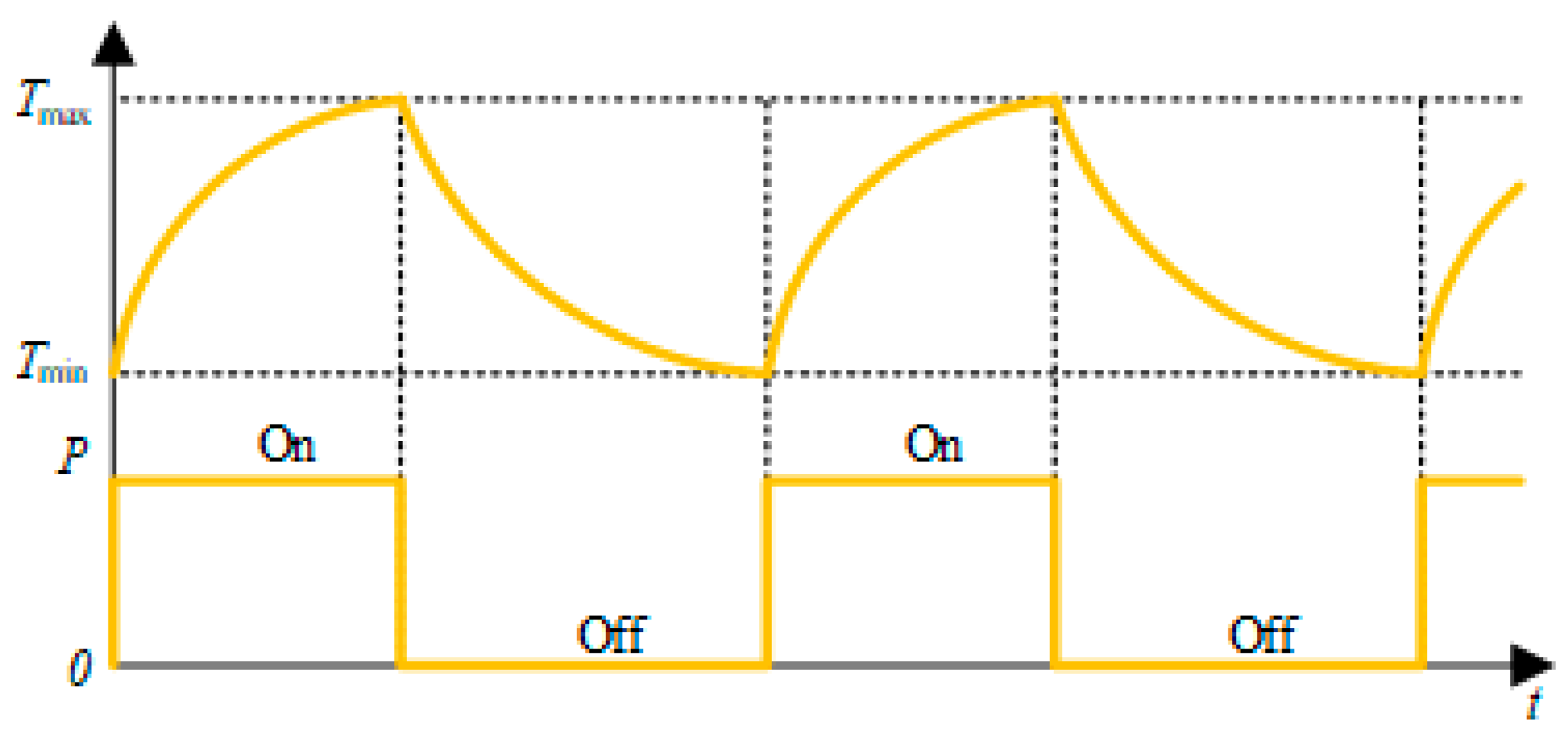
2.1. Temperature-Controlled Load ETP Model

The ETP model for direct heating was built to reflect the relationship between the temperature in the room and the wall, air, outdoor temperature, and other factors. The temperature-controlled load model studied in this paper is shown in Figure 1. In northern Chinese cities, especially in winter, temperature-controlled loads have a huge adjustable capacity due to their flexible scheduling and fast response. The scheduling and control of temperature-controlled loads benefit from the hardware advantages of the smart grid. Advanced Metering Infrastructure (AMI), with the full-speed development of communication information technology, has gradually become an indispensable and important part of the electric power field, which has a complete set of measurements. Collecting and analyzing the data processing system [15,16,17], the LA can obtain the start-and-stop status of the temperature-controlled loads and room temperatures as well as controlling the temperature-controlled loads of the users through the intelligent technology.

For temperature-controlled loads, the temperature in the room is related to the heat-producing power, heat-dissipating power, and heat-storage characteristics of the house, and the heat-producing power and the heat-dissipating power of the room of the temperature-controlled loads are represented by the following models:

$$Q_{\mathrm{D},t}={\eta }_{\mathrm{d}}\cdot p$$

(1)

$$Q_{\mathrm{S},t}={\displaystyle \sum _{i=1}^{n}K\cdot F}\left(T_{\mathrm{in},t}-T_{\mathrm{out},t}\right)$$

(2)

where η_d and p denote temperature-controlled load efficiency and power; n is the number of enclosure structures; K is the heat dissipation coefficient of the enclosure structures; F is the heat dissipation area of the structure; T_in,t and T_out,t are the temperatures inside the room and outside the room, at the time t.

For ease of presentation, the room equivalent thermal resistance R is introduced, and Equation (2) can be simplified to the following equation:

$$Q_{\mathrm{S},t}=\left(T_{\mathrm{in},t}-T_{\mathrm{out},t}\right)/R$$

(3)

According to the laws of thermodynamics, the heat-storage capacity Q_C,t of the room at time t can be expressed by Equation (4).

$$Q_{\mathrm{C},t}={\displaystyle \sum _1^{L}cm}\cdot B$$

(4)

where c is the value of the specific heat capacity of each type of material substance in the dwelling; m is the mass of each type of material substance in the dwelling; L is the number of categories of heat storage; B is the rate of change of temperature with the value of ΔT/Δt.

Since the occupants are more concerned about the indoor temperature change than the complexity of the thermal process of the building, the equivalent thermal parameter (heat capacity) is further introduced here to characterize the thermal storage properties of the indoor gases and solid materials, and the corresponding equations of the thermal parameter are shown in Equation (5).

$$Q_{\mathrm{C},t}=C\cdot B^{\ast }$$

(5)

where C is the equivalent heat capacity of the room; B* is the differential rate of change of temperature in the room with a value of dT/dt.

According to the law of conservation of energy, the amount of heat produced by the temperature-controlled load should be equal to the sum of the heat dissipated and stored in the indoor room, and the dynamic thermodynamic model of each room is finally obtained as shown in Equation (6):

$$C\frac{\mathrm{d}T}{\mathrm{d}t}={\eta }_{\mathrm{d}}\cdot p-\frac{T_{\mathrm{in},t}-T_{\mathrm{out},t}}{R}$$

(6)

To simplify the above model for ease of calculation, assuming that the air and wall temperatures in the room are the same during the same time period, the temperature in the room when the temperature-controlled load stops supplying heat and when it starts supplying heat is represented by the following model:

$$T_{\mathrm{in},t+1}=T_{\mathrm{out},t+1}-(T_{\mathrm{out},t+1}-T_{\mathrm{in},t})e^{-\Delta t/RC}$$

(7)

$$T_{\mathrm{in},t+1}=T_{\mathrm{out},t+1}+{\eta }_{\mathrm{d}}\cdot pR-\left(T_{\mathrm{out},t+1}+{\eta }_{\mathrm{d}}\cdot pR-T_{\mathrm{in},t}\right)e^{-\Delta t/RC}$$

(8)

Figure 2 shows the process of the dynamic change of temperature with temperature-controlled load start and stop. Without control, the temperature-controlled load starts and stops periodically within a certain temperature range. After the temperature-controlled load is turned on, it converts electrical energy into thermal energy, and the room temperature increases; conversely, the room temperature decreases, and when the room temperature drops to the lower temperature boundary, the temperature-controlled load starts again and begins the warming process, and so on and so forth. Considering that the human body’s comfort temperature is a zone, therefore, the room temperature can be maintained in the human body’s comfort temperature band. LA can control the temperature control load start and stop through direct control to make the room temperature stay within a certain limit.

Different occupants have variability in the perception of the ambient temperature; for the purpose of fitting the actual situation considerations, for a temperature interval that varies within a small range, the comfort of the occupants will not change significantly, so the occupants’ demand for indoor temperature has a certain limit. Based on this demand characteristic, the room temperature can be varied within this interval. This paper measures the subjective satisfaction of human body with hot and cold environments by the Predicted Mean Vote (PMV) of thermal sensation, so as to calculate the optimal thermal comfort of the occupants. The PMV is a comprehensive index that includes the parameters of indoor temperature, humidity, human body’s heat in clothing, and the activity state [18]. The PMV is mainly divided into seven categories to reflect the thermal sensation of the occupants. When the PMV value is 0, then the human body is most satisfied with the feeling of the ambient temperature [19,20,21].

$$\begin{array}{l}\mathrm{PMV}=(0{.303\mathrm{e}}^{-0.036M}+0.028\left)\right\{M-\sigma -3.05\times {10}^{-3}\cdot [5733-6.99(M-\sigma )-P_a]\hspace{0.33em}-\\ \hspace{0.33em}\hspace{0.33em}\hspace{0.33em}\hspace{0.33em}\hspace{0.33em}\hspace{0.33em}\hspace{0.33em}0.42[(M-\sigma )-58.15]-1.7\times {10}^{-5}\cdot M(5867-P_a)-0.0014\cdot M(34-T_{\mathrm{in}})-\\ \hspace{0.33em}\hspace{0.33em}\hspace{0.33em}\hspace{0.33em}\hspace{0.33em}\hspace{0.33em}\hspace{0.33em}3.96\times {10}^{-8}{f}_{\mathrm{clo}}[{(T_{\mathrm{clo}}+273)}^4-{(T_{\mathrm{r}}+273)}^4]-f_{\mathrm{clo}}{h}_{\mathrm{c}}(T_{\mathrm{clo}}-T_{\mathrm{in}})\}\end{array}$$

(9)

where M represents the energy metabolism rate of the human organism; σ is the activity rate of the human organism; P_a is the partial pressure of water vapor in the air; T_in is the room temperature (air temperature); f_clo is the heat of the human body in clothing; T_clo is the surface temperature of clothing; T_r is the average radiant temperature; h_c is the thermal conductivity. Based on existing studies, the formula for PMV can be simplified as follows [22]:

$$\mathrm{PMV}=a{T}_{\mathrm{in}}+b{P}_v-c$$

(10)

where T_in represents room temperature; P_v is the relative humidity of the room; a, b, and c represent already modeled parameters, respectively, related to the user’s own characteristics.

Due to the differences in age, health, and economic level of users, the switching status of temperature control equipment is affected by the comfort temperature range of different users. In this study, users were categorized into two groups based on their age: the young and the elderly. The two groups were then categorized into general and high-income groups based on their economic level. By means of a questionnaire survey of the occupants, statistical data such as the thermal resistance (TR) of the users’ clothing and activity intensity were collected, and finally the optimal comfort levels for different groups of people were calculated, as shown in

Table 1. PMV model parameters for different populations.

Type	TR	a	b	c	Optimal Temperature
The young	0.5	0.272	0.248	7.245	24
	1.0	0.242	0.614	5.587	24
The elderly	1.0	0.149	−0.107	2.640	26
	1.5	0.148	−0.137	2.524	24

. The detailed temperature design scheme is shown in Appendix A.

People with different incomes are affected by time-sharing tariffs and have different temperature requirements. For the economically well-off people, influenced by their work and social environment, they are generally active outdoors in the evening, while the working class, influenced by the nature of their work, live a regular life and are generally at home from 7 p.m. to 7 a.m.; for the elderly, they choose to go out during the daytime when the temperature is high outdoors, while they generally choose to stay indoors in the evening due to the cold outdoor temperature in the winter.

Utilizing the temperature-regulated load ETP model and the comfort temperature range, the temperature-controlled load on time ${\tau }_{\mathrm{on}}^t$, off time ${\tau }_{\mathrm{off}}^t$, and total control time ${\tau }_{\mathrm{c}}^t$ can be derived:

$${\tau }_{\mathrm{on}}^t=-Z\ln \frac{T_{\mathrm{out},t}+\eta pR-T_{\max ,t}}{T_{\mathrm{out},t}+\eta pR-T_{\min ,t}}$$

(11)

$${\tau }_{\mathrm{off}}^t=Z\ln \frac{T_{\mathrm{out},t}-T_{\max ,t}}{T_{\mathrm{out},t}-T_{\min ,t}}$$

(12)

$${\tau }_{\mathrm{c}}^t={\tau }_{\mathrm{off}}^t+{\tau }_{\mathrm{on}}^t$$

(13)

where Z = RC; ε = e^−1/RC; T_out,t is the outdoor temperature at time t; the maximum and minimum bounds of temperature comfort are T_max, T_min; η, p, R and C are the efficiency of electric heating, the power of electric heating, the thermal resistance of the room, and the thermal capacity of the room.

2.2. Temperature-Controlled Capacity

In this paper, the differences between the buildings were considered to make the temperature-controlled capacity prediction as close as possible to the actual results. Based on the classification of residential structures, the buildings were divided into three categories: superior buildings (SB), medium buildings (MB), and ordinary buildings (OB). Different buildings have different housing areas, so they have different thermal parameters and temperature-controlled load installed power.

The following is an example of a medium building to illustrate the rotational control process of temperature-controlled loads, and the control process of other types of buildings is similar and will not be repeated. The LA of the medium building counts the total number of temperature-controlled loads and aggregates them together to form a temperature-controlled loads group. The contract between the LA and the occupants stipulates that the temperature in the room will be controlled within the range of [T_min, T_max], and when the indoor temperature exceeds T_max, the LA controls the temperature-controlled loads to shut down; when the indoor temperature falls below T_min, the LA controls the temperature-controlled loads to start up. Assuming that the control time step of the temperature-controlled load is 10 min, the start-up time is 6 min, and the shutdown time is 4 min, we can obtain the state distribution table of the temperature-controlled load in one control cycle, as shown in

Table 2. Temperature-controlled load status table.

Time/min	Temperature-Controlled Load
	1	2	3	4	5	6	7	8	9	10
1	1	1	1	1	1	1	0	0	0	0
2	0	1	1	1	1	1	1	0	0	0
3	0	0	1	1	1	1	1	1	0	0
4	0	0	0	1	1	1	1	1	1	0
5	0	0	0	0	1	1	1	1	1	1
6	1	0	0	0	0	1	1	1	1	1
7	1	1	0	0	0	0	1	1	1	1
8	1	1	1	0	0	0	0	1	1	1
9	1	1	1	1	0	0	0	0	1	1
10	1	1	1	1	1	0	0	0	0	1
11	1	1	1	1	1	1	0	0	0	0
12	0	1	1	1	1	1	1	0	0	0
13	0	0	1	1	1	1	1	1	0	0
14	0	0	0	1	1	1	1	1	1	0
15	0	0	0	0	1	1	1	1	1	1
16	1	0	0	0	0	1	1	1	1	1
17	1	1	0	0	0	0	1	1	1	1
18	1	1	1	0	0	0	0	1	1	1
19	1	1	1	1	0	0	0	0	1	1
20	1	1	1	1	1	1	0	0	0	0

(1 is on, 0 is off).

At any time, the proportion of temperature-controlled loads that are in the unopened state is τ_off/τ_c, so at moment t, the temperature-controlled capacity available to LA is shown in Equation (14) as follows:

$$P_{\mathrm{LA},t}={\displaystyle \sum _{i=1}^3\frac{{\tau }_{\mathrm{off}}^t}{{\tau }_{\mathrm{c}}^t}\cdot np}$$

(14)

where n represents the count of temperature-controlled loads; p denotes the temperature-controlled load power.

2.3. Time-Shiftable Capacity

The proportion of each type of load on a given day in a Chinese city is shown in Figure 3. It is not difficult to find that residential loads account for 30% of the peak loads, and 2/3 of this portion belongs to the time-shiftable loads that can be grid-friendly. Time-shiftable residential loads exist in the existing power system on a large scale and account for a large proportion of the load. Based on the consideration of temperature-controlled capacity, the transfer of this part of time-shiftable capacity can make the excess new energy, such as abandoned wind and light, fully consumed, simultaneously enhancing the operational economy of the system, which is a high-quality regulating resource in the optimal scheduling of microgrids.

In one city, for example, 80.4% of users are willing to change their electricity consumption habits during peak periods. In China, the residents have controllable loads of electricity equipment as shown in Figure 4, of which the loads with the largest share are water heaters, air conditioner, and dishwashers [23]. However, this study takes a northern Chinese city as an example, so the air conditioning load is not considered.

In this paper, water heaters, dishwashers and washing machines are selected as the time-shiftable loads and the power usage patterns of the three types of loads are shown in

Table 3. Parameters of time-shifted loads.

Type	Water Heater	Dishwasher	Washing Machine
Power value/kW	[2, 1.6, 1.2]	0.8	[0.5, 0.2]
Duration/h	[1, 1, 1]	1	[1, 1]

, which can be used in accordance with the operating demand of the power system by adjusting the opening time of the loads to transfer their own power hours. The total amount of this type of load remains unchanged for the entire operating cycle before and after the occurrence of the transfer, and so the power consumption period will not affect the user’s power consumption demand.

The intended purpose of load shifting is to turn on most of the loads in the low-tariff case and fewer loads in the high-tariff case during the optimization cycle. The time-shifted capacity can be described using the following model:

$$P_{\mathrm{tr},t}=P_{\mathrm{pre},t}+P_{\mathrm{in},t}-P_{\mathrm{out},t}$$

(15)

where P_tr,t is the time-shifted capacity of time t after load transfer; P_pre,t represents the power consumption at time t predicted before load transfer; P_in,t and P_out,t denote the load power that can be transferred into time t from other time and the load power that can be transferred out of time t to other time. P_in,t and P_out,t can be articulated by the following equation:

$$P_{\mathrm{in},t}={\displaystyle \sum _{\begin{array}{c}t\prime =1\\ t\prime \ne t\end{array}}^T{\displaystyle \sum _{k=1}^{K_1}{x}_{k,t\prime ,t}}}\cdot p_{1,k}+{\displaystyle \sum _{h=1}^H{\displaystyle \sum _{\begin{array}{c}t\prime =1\\ t\prime \ne t-h\end{array}}^T{\displaystyle \sum _{k=1}^{K_2}{x}_{k,t\prime ,(t-h)}}}}\cdot p_{(h+1),k}$$

(16)

$$P_{\mathrm{out},\mathrm{t} }={\displaystyle \sum _{\begin{array}{c}t″=1\\ t″\ne t\end{array}}^T{\displaystyle \sum _{k=1}^{K_1}{x}_{k,t,t″}}}\cdot p_{1,k}+{\displaystyle \sum _{h=1}^H{\displaystyle \sum _{\begin{array}{c}t″=1\\ t\prime \prime \ne t-h\end{array}}^T{\displaystyle \sum _{k=1}^{K_2}{x}_{k,(t-h),t″}}}}\cdot p_{(h+1),k}$$

(17)

where K₁ represents the number of categories of time-shiftable loads; K₂ represents the number of categories of time-shiftable loads for which the power usage period is greater than one scheduling cycle; H is the maximum runnable time for time-shiftable loads; T is the total system optimization time; x_k,t′,t denotes the number of time-shiftable loads of category k; p_1,k denotes the power demand of time-shiftable loads of category k in the first run-time period; p_1+h,k denotes the power demand of time-shiftable loads of category k in the h + 1 run-time period.

The aim of this paper is to allow the utilization of all types of energy in the microgrid by changing the time-shifted loads’ power consumption periods while the total amount of all categories of loads remains constant. The load profile after load shifting occurs fits the target load profile as closely as possible. The preceding issue can be depicted by the subsequent model:

$$\min {\displaystyle \sum _{t=1}^T{\left(P_{\mathrm{tr},t}-P_{\mathrm{obj},t}\right)}^2}$$

(18)

3. A Bi-Level Scheduling Model for Microgrids with Satisfaction Consideration

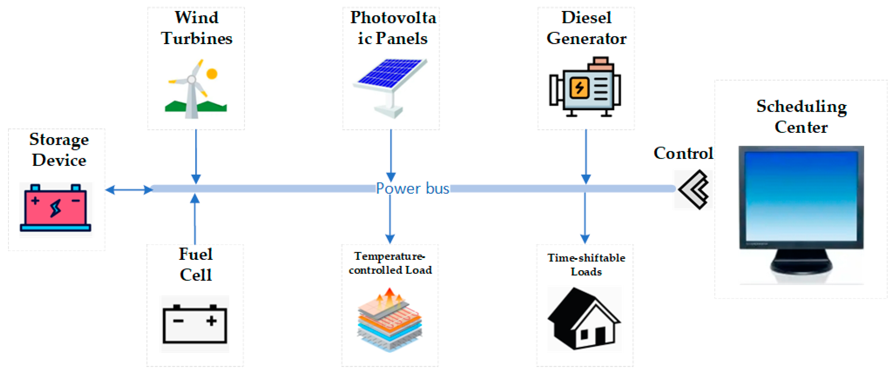
3.1. Overall Composition of the Microgrid

The detailed configuration of the microgrid investigated in this paper is illustrated in Figure 5, where the arrows indicate the direction of power flow.

This paper uses a microgrid system that includes generating units such as wind turbines (WTs), photovoltaic cells (PVs), diesel generators (DEs), and fuel cells (FCs), as well as temperature-controlled loads, time-shiftable loads, and energy storage devices (ESs).

3.2. Objective Function

3.2.1. Upper-Level Optimization Model

The consumption of renewable energy leads to changes in the way users use electricity, which in turn affects the users’ electricity consumption. Therefore, this paper selects a microgrid cycle’s (24 h) temperature-controlled loads and time-shiftable loads of integrated satisfaction as a measure of the residents’ preference for electricity, and as an indicator of higher satisfaction, indicating that households pay more attention to their own habits of electricity consumption and higher consumption capacity. The objective function can be expressed as the following equation:

$$\max f_1=\left[{\omega }_1\zeta +{\omega }_{2}s\right]$$

(19)

where ζ is the temperature-controlled load electricity consumption satisfaction; s is the time-shiftable load electricity satisfaction; ω₁ and ω₂ are the weight indices of electricity bill satisfaction and electricity satisfaction, respectively, and ω₁ + ω₂ = 1, which reflects the residents’ tendency to the load type [24].

Satisfaction with the cost of electricity is the size of the difference between the customer’s current cost of electricity and the original cost of electricity. The larger the difference, the lower the satisfaction; the smaller the difference, the greater the satisfaction. The formula for calculating the satisfaction of temperature-controlled load electricity consumption is outlined below:

$$\zeta =1-\frac{D-D_0}{D_0}$$

(20)

where D₀ denotes the expenditure cost of electric heating when peak and valley tariffs are not implemented; D denotes the expenditure cost of electric heating when peak and valley tariffs are implemented. The expressions for D₀ and D are outlined below:

$$\left\{\begin{array}{l}D={\displaystyle {\int }_{T_{\mathrm{p}}}{v}_{\mathrm{p}}{P}_{t}dt+{\displaystyle {\int }_{T_{\mathrm{s}}}{v}_{\mathrm{s}}{P}_{t}dt}+{\displaystyle {\int }_{T_{\mathrm{v}}}{v}_{\mathrm{v}}{P}_{t}dt}}\\ D_0={\displaystyle {\int }_T{v}_0{P}_{i0}}\end{array}\right.$$

(21)

Satisfaction with electricity use is the deviation value of the user’s existing electricity use habit from the original electricity use habit. The larger the deviation value, the lower the satisfaction with electricity consumption; the smaller the deviation value, the higher the satisfaction with electricity consumption. The time-shiftable load electricity satisfaction formula is outlined below:

$$s=1- \frac{{\displaystyle {\int }_T\left|P_{\mathrm{tr},t}-P_{\mathrm{pre},t}\right|\mathrm{d}t}}{{\displaystyle {\int }_T{P}_{\mathrm{tr},t}\mathrm{d}t}}$$

(22)

where the value of s is in the range of [0, 1], and the value of s is 1 when the satisfaction of electricity consumption is the maximum, which reflects the change in the time-shiftable load consumption curve as well as the increase or decrease in electricity consumption.

3.2.2. Lower-Level Optimization Model

In this paper, economic scheduling of microgrids is achieved by using the flexible resources on the load side, with the objective function of maximizing the gain from the operation of the entire microgrid.

$$\max f_2={\displaystyle \sum _{t=1}^T\left[R_{\mathrm{all},t}-C_{\mathrm{all},t}\right]}$$

(23)

where T is the total optimization period; C_all,t denotes the total cost of the operation of the whole microgrid system; R_all,t denotes the total benefit of the operation of the whole microgrid system.

3.2.3. Total Social Benefit Functions

User satisfaction is of increasing importance in power systems, especially for temperature-controlled loads and time-shiftable loads, where factors such as users’ usage habits, comfort requirements, and cost affordability have a direct impact on their satisfaction. If the scheduling strategy of temperature-controlled loads and time-shiftable loads can fully take into account the preferences and needs of users, it can not only enhance user satisfaction and participation, but also help microgrids to better balance supply and demand through demand-side management and improve the overall operational efficiency of the system.

Microgrid benefits mainly emphasize the efficient use of energy and the economy of system operation, covering cost minimization (power generation, operation, maintenance costs, etc.), energy consumption optimization (improving energy use efficiency), and environmental impact minimization (reducing carbon emissions). In microgrids, how to maximize cost-effectiveness while ensuring a stable and reliable power supply is a key issue in design and scheduling.

In the microgrid scheduling model, two weight coefficients are introduced to reflect the prioritization of microgrid benefits and user satisfaction. Focus on the benefits of the microgrid means scheduling more users of the controllable load, which creates greater differences between the current and original power habits of the user, which leads to a reduction in user satisfaction; focus on the user’s experience of electricity means that the user’s experience of electricity is at the core; as far as possible, the user’s original habits with electricity should not change, which will make the wind power and photovoltaic power generation eliminate the decrease, resulting in a reduction in the benefits of the microgrid. It not only considers the goal of realizing the efficient operation of microgrids from technical and economic perspectives, but also gives full consideration to user needs and experiences. The total social benefit function is shown in the following equation:

$$R_{\mathrm{to}}=\beta f_1+\gamma f_2$$

(24)

where β and γ denote the weighting coefficients of satisfaction and microgrid profit, respectively; β + γ = 1, when β > γ, which means that at that time, more attention is paid to the user’s experience of electricity consumption; while when β < γ, it means that at that time, more attention is paid to the microgrid’s profitability.

3.3. Constraints

3.3.1. Power Equilibrium Constraint

Equation (23) denotes that power generation and consumption are balanced at all times within the microgrid.

$${\displaystyle \sum _{i=1}^N{P}_{i,t}}+P_{\mathrm{ES},t}+P_{\mathrm{grid},t} =P_{\mathrm{LA},t}+P_{\mathrm{tr},t}-P_{\mathrm{PV},t}-P_{\mathrm{WT},t}$$

(25)

where P_WT,t, P_PV,t, P_LA,t, and P_tr,t are the power of WT, PV, temperature-controlled capacity, and time-shifted capacity at time t, respectively.

3.3.2. Upper and Lower Temperature Constraints

Room temperature is maintained in a range when the temperature-controlled load is switched on:

$$T_{\min }\le T_t\le T_{\max }$$

(26)

3.3.3. Transfer Time and Volume Constraints

The following constraints are placed on the time-shiftable loads, ensuring the stable and reliable operation of the system as well as the unchanged total load before and after the shift:

$$\left\{\begin{array}{ll}\forall t\prime <s_{k,t},\hfill & x_{k,t,t\prime }=0\hfill \\ \forall t\prime >\left(s_{k,t}+d_{k,t}\right),\hfill & x_{k,t,t\prime }=0\hfill \end{array}\right.$$

(27)

where s_k,t is the earliest time at which the shift occurs; d_k,t is the shift time margin for a time-shiftable load of category k.

$$\left\{\begin{array}{l}\forall t,t\prime ,k\hspace{1em}{x}_{k,t,t\prime }\ge 0\hfill \\ x_{k,t}={\displaystyle \sum _{t\prime =1}^T{x}_{k,t,t\prime }}\hfill \end{array}\right.$$

(28)

where x_k,t represents the count of time-shiftable loads of category k in time-of-use time period t before load shifting.

3.3.4. Renewable Energy Output Constraints

The renewable energy output constraints include mainly wind power output and photovoltaic output constraints:

$$\left\{\begin{array}{l}{P}_{\mathrm{WT},\min }\le P_{\mathrm{WT},t}\le P_{\mathrm{WT},\max }\\ P_{\mathrm{PV},\min }\le P_{\mathrm{PV},t}\le P_{\mathrm{PV},\max }\end{array}\right.$$

(29)

where P_WT,max, P_WT,min, P_PV,max, and P_PV,min are the upper and lower bounds of WT and PV output power, respectively.

3.3.5. Micro-Power Output Constraints

The constraints mainly include diesel engine output constraints and micro gas turbine output constraints:

$$P_{\mathrm{i},\min }\le P_{\mathrm{i},t}\le P_{\mathrm{i},\max }$$

(30)

where Pi,min and Pi,max are the maximum and minimum values of DE and FC output power, respectively.

3.3.6. Storage Battery Operating Constraints

The operating constraints of the SB encompass limitations on charging and discharging states as well as output power:

$$\left\{\begin{array}{l}{S}_{\mathrm{SOC},\min }\le S_{\mathrm{SOC},\mathrm{t}}\le S_{\mathrm{SOC},\max }\\ \frac{-0.2E_{\mathrm{ES}}}{\Delta t}\le P_{\mathrm{ES},t}\le \frac{0.2E_{\mathrm{ES}}}{\Delta t}\end{array}\right.$$

(31)

where S_SOC,min and S_SOC,min are the limits of the energy storage device’s state of charge, respectively; Δt is the scheduling time step; and E_ES is the energy storage device capacity.

3.4. Solving Methods

Solving bi-level optimization problems is generally achieved by using the Karush-Kuhn-Tucker (KKT) condition. The KKT condition is an important tool in the field of nonlinear programming for finding the necessary conditions for the optimal solution of an optimization problem. Both objective functions to be optimized in this paper are to obtain the maximum value, which is transformed into a minimum value problem by taking the negative sign in the solution process. For a two-layer model containing inequalities and equation constraints, the upper layer model is expressed as the following equation:

$$\begin{array}{l}\min f_1(x,p)\\ \mathrm{s}.\mathrm{t}. \hspace{1em}{G}_a(x,p)\le 0(a=1,2,\cdots ,c)\\ \hspace{0.33em}\hspace{0.33em}\hspace{0.33em}\hspace{0.33em}\hspace{0.33em}\hspace{0.33em}{H}_b(x,p)=0(b=1,2,\cdots ,d)\end{array}$$

(32)

where G_a(x,p) and H_b(x,p) correspond to the inequality and equation constraints in the upper model, respectively.

The lower-level model is expressed as the following equation:

$$\begin{array}{l}\min f_2(p)\\ \mathrm{s}.\mathrm{t}. \hspace{1em}{g}_i(p)\le 0(i=1,2,\cdots ,m)\\ \hspace{0.33em}\hspace{0.33em}\hspace{0.33em}\hspace{0.33em}\hspace{0.33em}\hspace{0.33em}{h}_j(p)=0(j=1,2,\cdots ,n)\\ x\in X,\hspace{1em}p\in P\end{array}$$

(33)

where g_i(p) and h_j(p) correspond to the inequality and equation constraints in the lower model, respectively.

Through the KKT condition, the lower-level objective function is transformed to the following equation:

$$\begin{array}{l}\frac{d{f}_2}{dp}+{\displaystyle \sum {\lambda }_i}\frac{d{g}_i}{dp}+{\displaystyle \sum {\mu }_j}\frac{d{h}_j}{dp}=0\\ (p)\le 0,\hspace{1em}{\lambda }_i\ge 0,\hspace{1em}{\lambda }_i{g}_i(p)=0\\ h_j(p)=0,\hspace{1em}{\mu }_j\ne 0\\ p\in P\end{array}$$

(34)

Combining Equations (30) and (32) allows the original two-layer optimization problem to be transformed into a single-layer optimization problem, The optimal solution to the original problem can be obtained by simply solving the following equation:

$$\begin{array}{ll}\min \hfill & F(x,p)\hfill \\ \mathrm{s}.\mathrm{t}. \hfill & G_a(x,p)\le 0,\hspace{1em}{H}_b(x,p)=0\hfill \\ \hfill & \frac{d{f}_2}{dp}+{\displaystyle \sum {\lambda }_i}\frac{d{g}_i}{dp}+{\displaystyle \sum {\mu }_j}\frac{d{h}_j}{dp}=0\hfill \\ \hfill & g_i(p)\le 0,\hspace{1em}{\lambda }_i\ge 0,\hspace{1em}{\lambda }_i{g}_i(p)=0\hfill \\ \hfill & h_j(p)=0,\hspace{1em}{\mu }_j\ne 0\hfill \\ \hfill & x\in X,\hspace{1em}p\in P\hfill \end{array}$$

(35)

4. Simulation Analysis

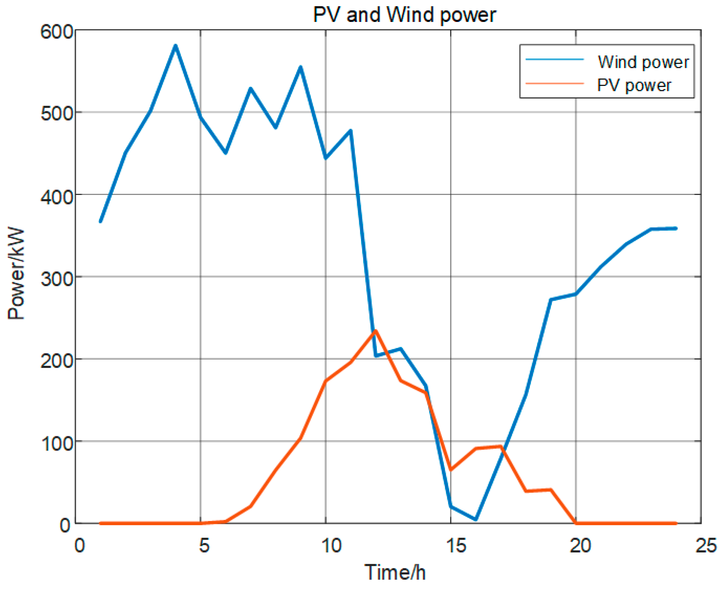
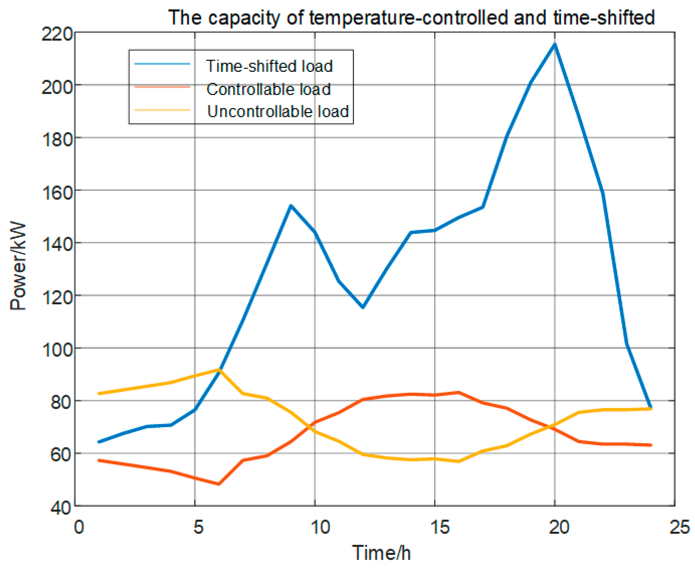
4.1. Experimental Settings

In order to verify the validity of the proposed method, the wind, solar, and load data were obtained from the real data of typical winter days in the Xinjiang Uygur region. Taking three communities in the Xinjiang Uygur Autonomous Region as examples, the levels of the three communities are ordinary, medium, and high, respectively. One building in each community was selected as the experimental building, and the temperature of each room was tested by a thermometer for 24 h, while the remote-control system was used to control the opening and closing of the temperature control equipment. Combining the indoor temperature and outdoor temperature, the thermal parameters of the house were obtained by parameter fitting. The temperatures and thermal parameters of the three types of rooms are shown in Appendix A. A visit to the neighborhood revealed that the ratio of younger to older age groups was roughly 6:4.

In this study, an islanded microgrid was selected, consisting of wind turbines, photovoltaic panels, diesel engines, fuel cells, energy storage units, temperature-controlled loads, and time-shiftable loads. The capacity of the energy storage device in the system was 100kW-h and the fuel cell was a proton exchange membrane fuel cell [25]. The pollutants in the system were CO₂, SO₂, and NO_X [26]. The parameter configurations are displayed in Appendix A. The interactive tariffs are based on time-of-day tariffs with a 24 h dispatch cycle and a 1 h unit dispatch time. In this study, MATLAB 2022b simulation software was employed to simulate one day’s PV and wind power generation, along with load data, as depicted in Figure 6 and Figure 7.

Simulations were carried out on MATLAB software using Yalmip 0.9.7 and the proposed distributed control problem was solved using the CPLEX solver 12.10.0 on a PC with a 11th Gen Intel(R) Core i7-11700 @ 2.50 GHz and 16 GB RAM. All the linearized models and constraints created were encoded in the required Yalmip 0.9.7 format in MATLAB software, after which Yalmip 0.9.7 was used to transform the encoded optimization problem into a computer program that could be recognized and solved by CPLEX solver 12.10.0.

The tariff periods in this paper are categorized as follows: peak hours are 11:00–14:00 and 18:00–21:00; flat hours are 07:00–11:00, 14:00–18:00, and 21:00–23:00; valley hours are 00:00–07:00 and 23:00–24:00. The time-of-day tariffs are presented in

Table 4. Time-of-use tariffs.

	Period	Tariff
Peak	11:00–14:00 18:00–21:00	0.3
Flat	07:00–11:00 14:00–18:00 21:00–23:00	0.2
Valley	00:00–07:00 23:00–24:00	0.1

.

To validate the economic viability and efficacy of the proposed day-ahead scheduling model, this paper sets up four comparison scenarios:

(1)

No temperature-controlled capacity and no time-shifted capacity in the microgrid;

(2)

Time-shifted capacity but no temperature-controlled capacity in the microgrid;

(3)

Temperature-controlled capacity but no time-shifted capacity in the microgrid;

(4)

Temperature-controlled capacity and time-shifted capacity in the microgrid.

4.2. Effectiveness Analysis of the Proposed Method

The final results of these four scenarios are shown in

Table 5. Results for each scenario.

Scenario Type	TL	SL	Microgrid Benefits/CNY	Consumption
1	/	/	178.15	53.02%
2	/	√	252.00	69.69%
3	√	/	259.24	71.32%
4	√	√	327.43	83.55%

, and it can be seen that the addition of TL and SL gradually improves the efficiency of the whole microgrid system and significantly increases the rate of new energy consumption.

4.3. Scheduling Results

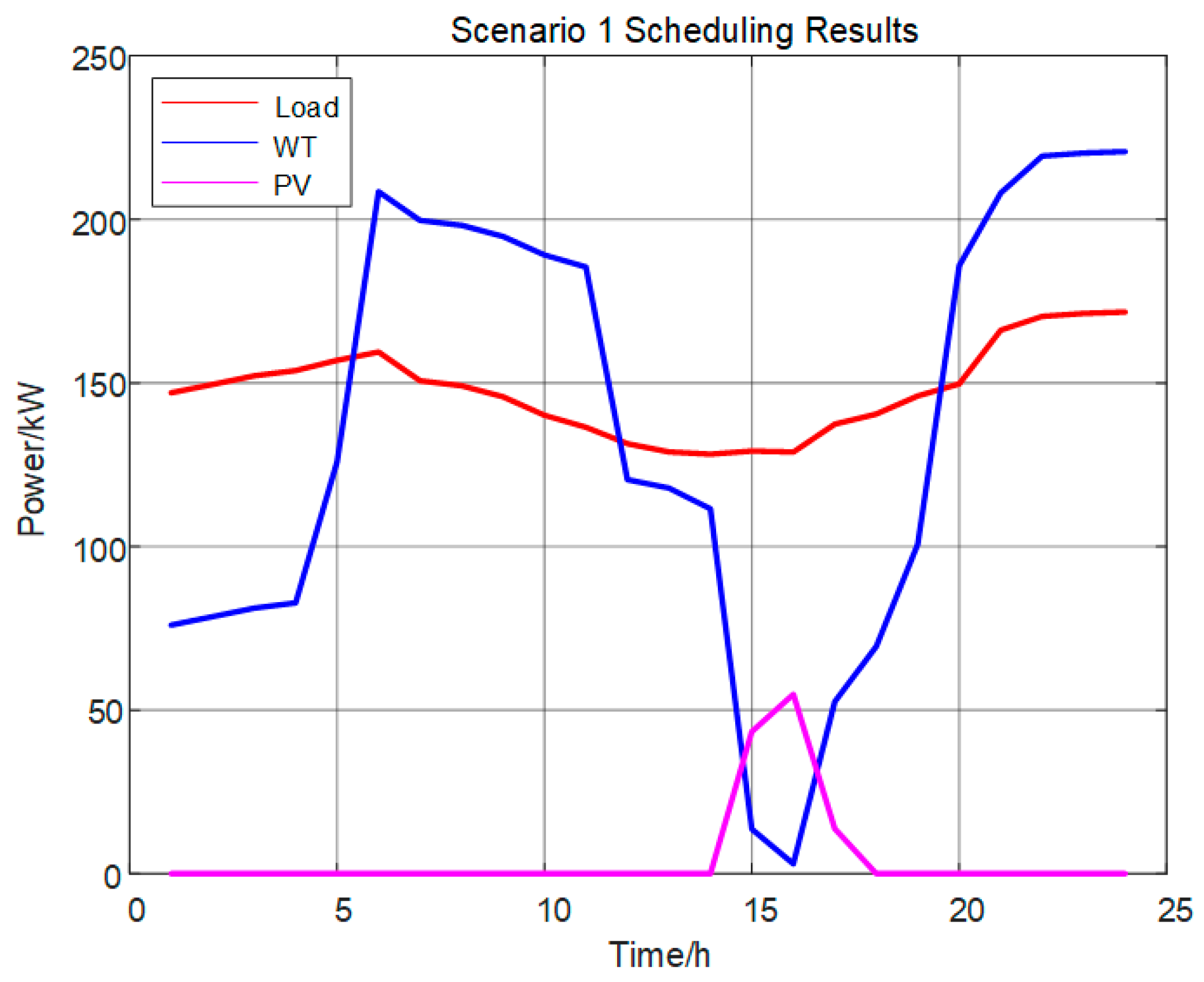
4.3.1. Scenario 1 Scheduling Results

The scenarios set up in this paper are all in island mode, where the proportion of clean energy is large, and the degree of matching between load and power output determines the economic performance of the whole microgrid operation. As shown in Figure 8, because the temperature-controlled capacity and time-shifted capacity are not involved in the scheduling of the microgrid system, the peaks and valleys of the grid are obvious, the new energy abandonment of the whole system is serious, and the microgrid economy is inferior.

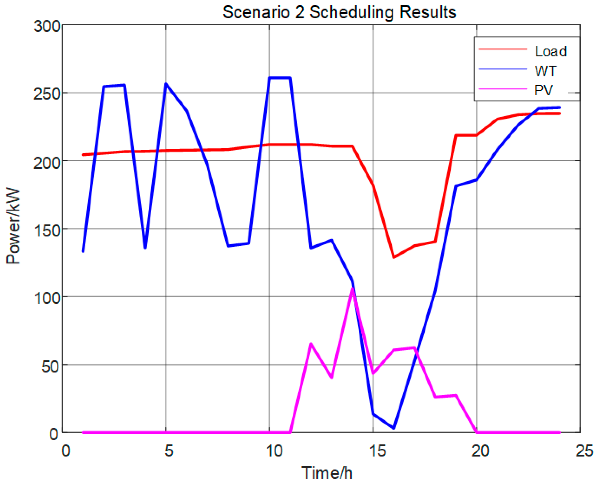
4.3.2. Scenario 2 Scheduling Results

As shown in Figure 9, after shifting the capacity to participate in the scheduling optimization, the system load value rises during the period of abundant PV generation, and the load curve is close to the new energy output curve. At the same time, the peak value of the load curve is shifted downward, but during the nighttime, it does not have any obvious advantage for wind power consumption. It can be seen that the addition of time-shifted capacity plays a partial role in shifting the peak value and promoting new energy consumption.

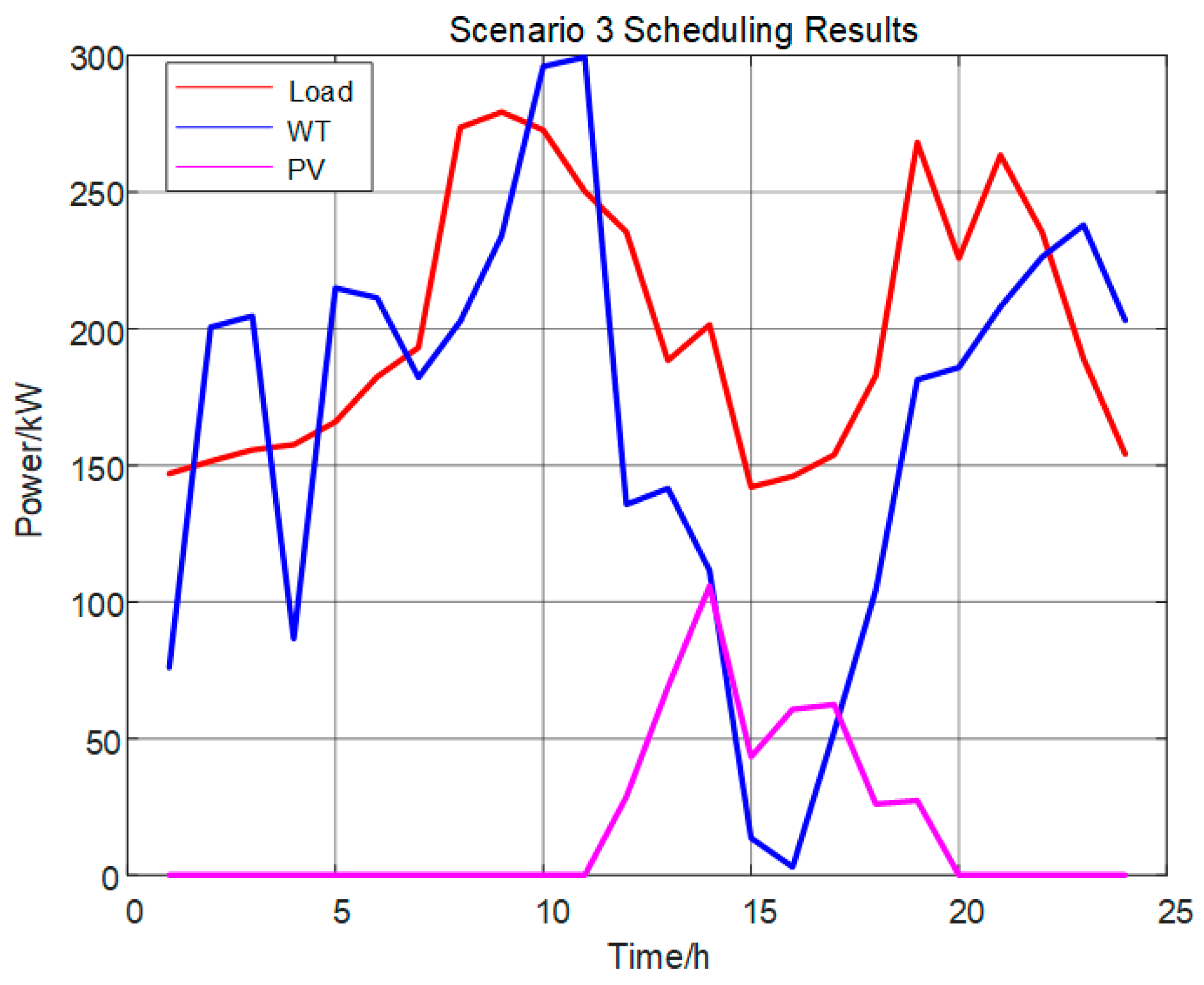
4.3.3. Scenario 3 Scheduling Results

As can be seen from Figure 10, after the temperature-controlled capacity is involved in the dispatch optimization, the match between the load profile and the new energy output is significantly improved in the nighttime period. The wind power output jumps from 77 kW to 137 kW between midnight and morning, and the wind power output is better than that in Scenario 2, while the photoelectricity consumed during the photovoltaic power period is obviously higher than that in Scenario 2, which promotes the new energy consumption during the whole scheduling cycle and reduces the abandoned power of wind and light.

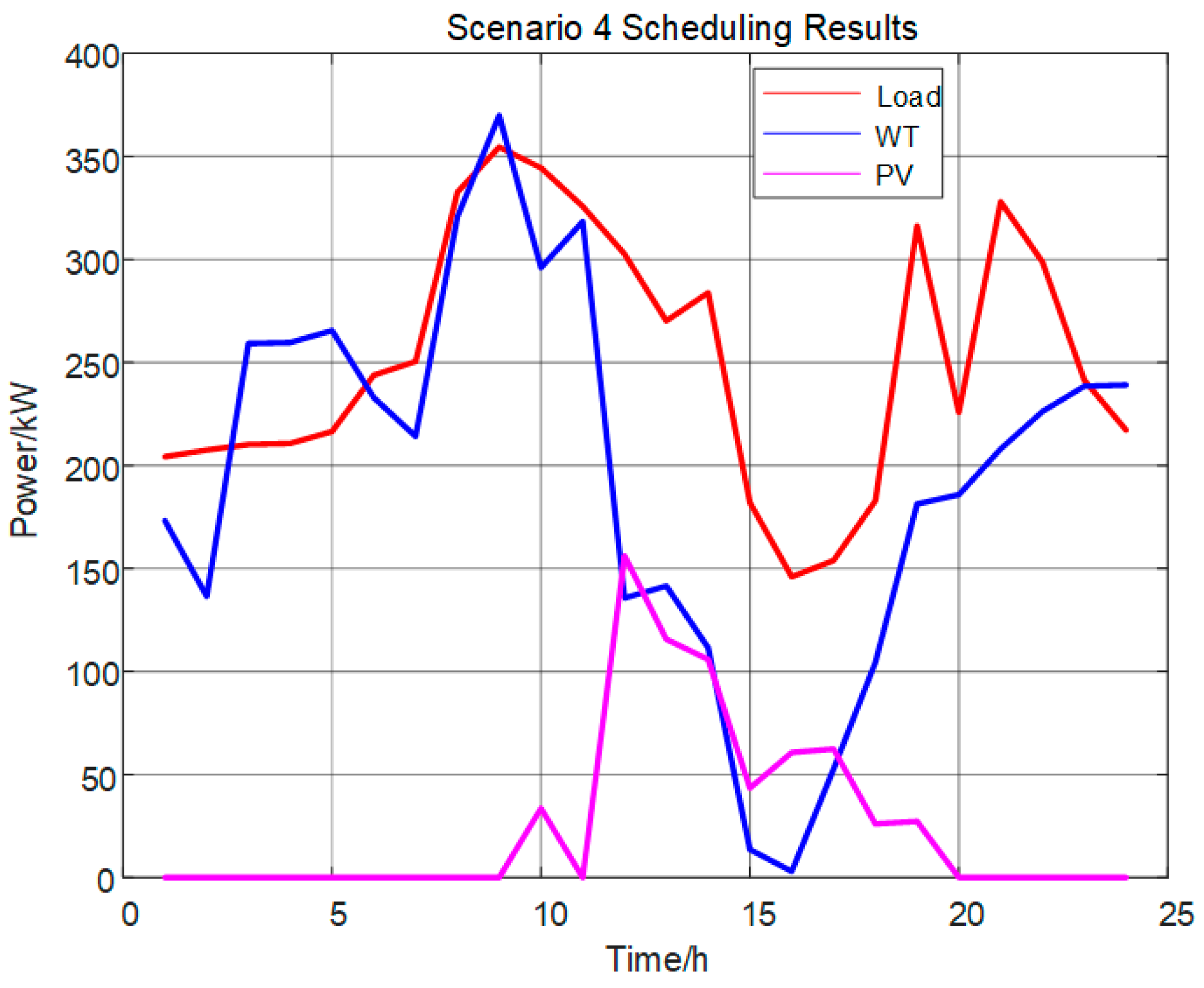
4.3.4. Scenario 4 Scheduling Results

As can be seen from Figure 11, compared with Scenario 1, a high proportion of power generated from new energy is consistently consumed both at night and during the daytime, taking into account the temperature-controlled capacity and time-shifted capacity. Compared with Scenarios 2 and 3, the optimized source-side and load-side matching is higher. It can be seen that the microgrid in the islanded state, taking into account the temperature control capacity of electric heating and the time-shiftable load, makes the operation of the whole system more cost-effective and efficient, and at the same time has a higher proportion of new energy consumption. The results of the dispatch of electrical energy are shown in Figure 12.

4.4. Temperature-Controlled Capacity and Time-Shifted Capacity Analysis

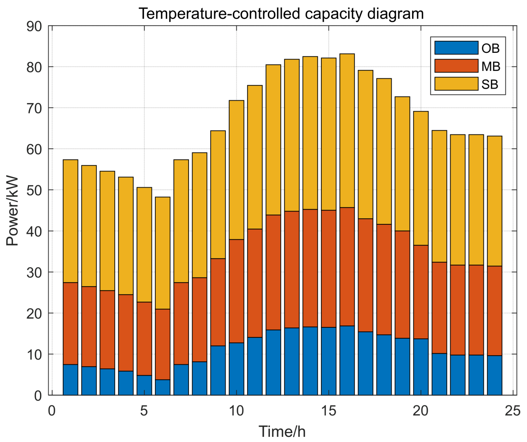
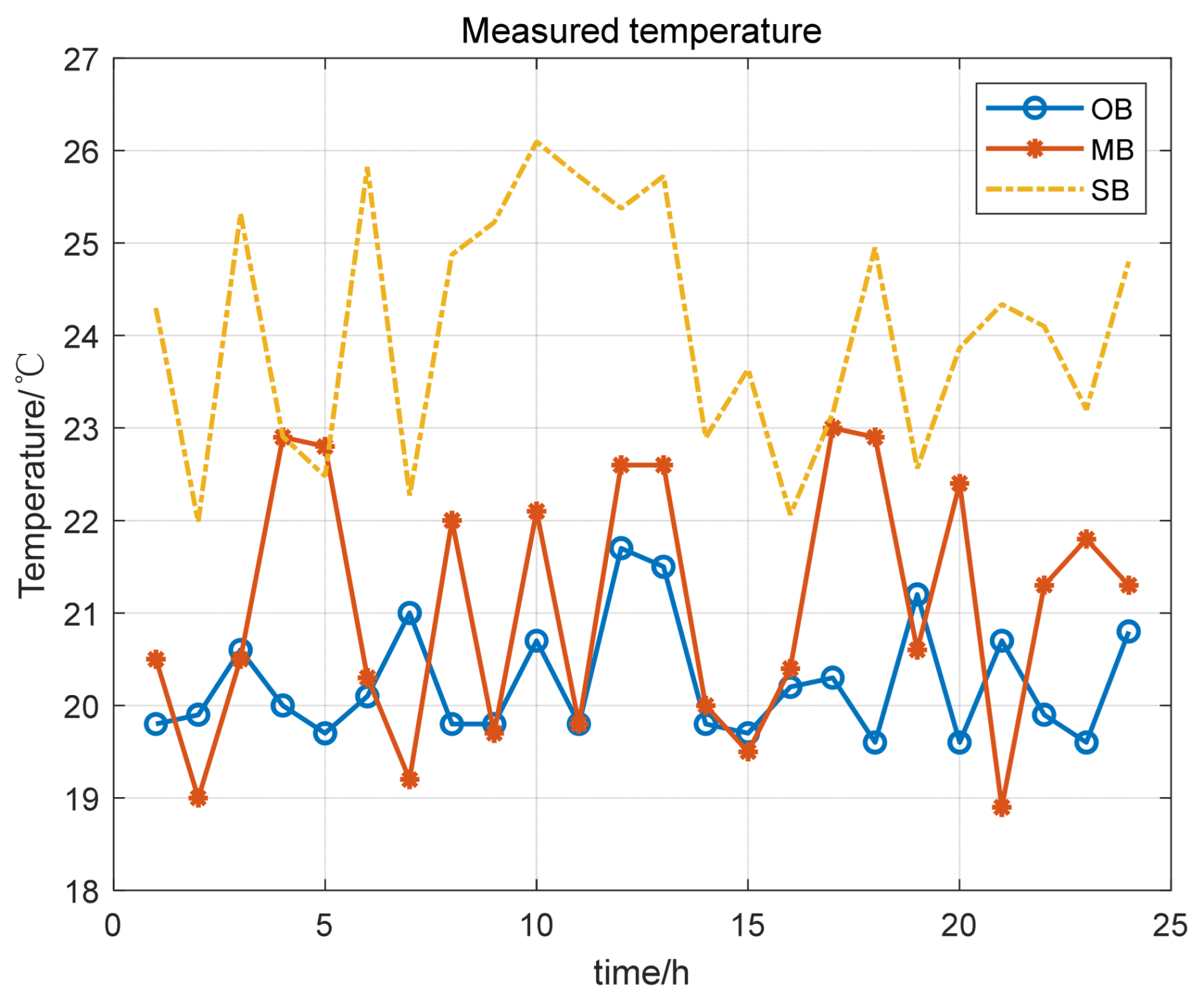
4.4.1. Temperature-Controlled Capacity Analysis

The temperature-controlled capacity available for scheduling varies due to the characteristics of the large temperature difference in winter. As can be seen from Figure 13, during the peak daytime period (6 a.m.–3 p.m.), as the outdoor temperature gradually rises with the sunshine, and then the room temperature rises, the temperature-controlled capacity of each building increases, and reaches an extreme value at 3 p.m.; from 3 p.m. to 8 p.m., the outdoor temperature gradually decreases with sunset, and the temperature-controlled loads that are controlled and turned on gradually increase under the synergistic cooperation between the LA and the users, and the temperature-controlled capacity also decreases. Between 8 p.m. and midnight, the total temperature-controlled capacity decreases to a lower level because the occupants have an immediate need for thermal comfort as the night temperature plummets.

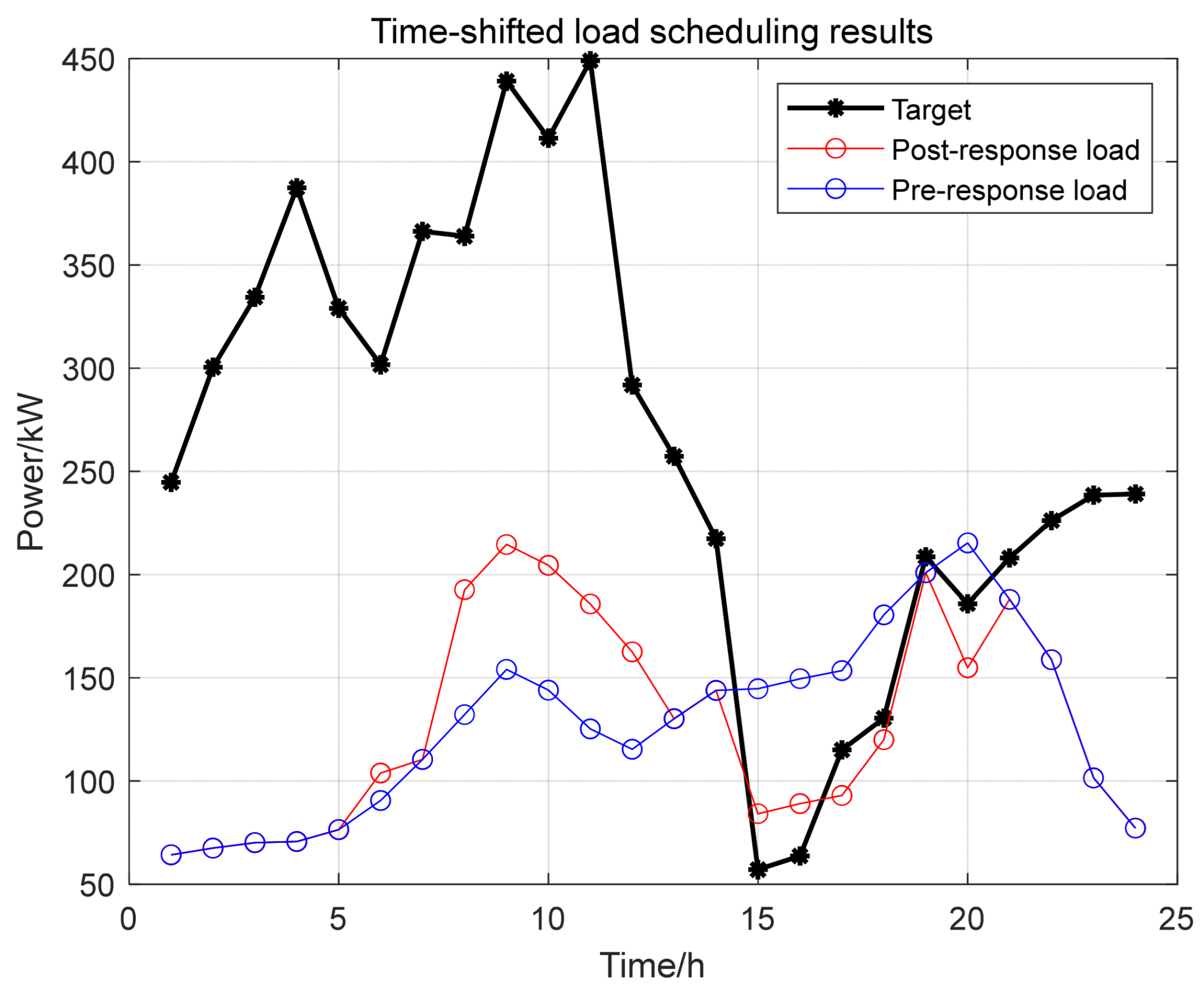
4.4.2. Time-Shifted Capacity Analysis

Since the microgrid operates in islanding mode, the proportion of power provided by new energy sources is high, so the sum of wind and PV outputs will be higher than the value of electricity load demand in some moments. By taking the power generated from wind power and PV as the target capacity curve, the time-shifted capacity result of the microgrid is shown in Figure 14, which shows that the time-shifted capacity during the period of scarcity of wind and solar power generation (time period 14–18 and 19–21) is shifted to the period of abundance of wind and solar power generation (time period 7–13), and the matching between the power source and the load is strengthened, and as a result, the amount of renewable energy consumed by the whole system can be improved.

4.5. Impact of Different Levels of Satisfaction

Because of the existence of the scheduling load, a trade-off needs to be made between microgrid benefits and total satisfaction, and the impact of the different weights of the two needs to be analyzed in the context of the optimal scheduling described above, using different weighting coefficients, as shown in

Table 6. Social benefits of different weightings.

Microgrid Benefits	Satisfaction	Social Benefits/CNY
0.3	0.7	194.78
0.5	0.5	347.41
0.7	0.3	499.84

. It can be seen that when households pursue comprehensive electricity satisfaction, the total social benefits are smaller when the consumption capacity of households is higher, and the importance of microgrid operating costs is lower; when priority is given to microgrid revenue, the total social benefits are larger when the user’s electricity habits are sacrificed, but this will also incentivize LA to guide the user to participate in the demand response, which will lead to the bursting out of more demand response potential.

5. Conclusions

In this paper, we propose a temperature-controlled capacity model and a time-shifted capacity model in terms of LA and study the optimal scheduling of microgrids, mainly from the three aspects of distributed power sources, customers’ comprehensive electricity satisfaction, and load-side resource regulation. The scheduling results of the arithmetic example show that:

(1)

Synthesizing the respective characteristics of the population, the decentralized temperature-controlled loads of different types of residences are aggregated to form a considerable scale of temperature-controlled capacity through the rotation control strategy, which makes the results more reasonable and realistic; the regulation potential of a large number of commonly used time-sharing loads on the user side is utilized through the time-sharing scheduling strategy, which creates time-sharing capacity to participate in the scheduling.

(2)

After clustering the two types of loads to form a significant demand response resource, the effectiveness of the model was tested by the measured data in the Xinjiang Uygur Autonomous Region. The results show that the model improves the overall economy of microgrid operation, reduces the peak-to-valley gap of the microgrid system, and greatly improves the new energy consumption rate and the total social benefits.

(3)

A comprehensive electricity satisfaction model is used to represent the consumption preferences of residents and also to analyze their impact on the economic efficiency of the microgrid. Favoring comprehensive satisfaction will result in the loss of social benefits, and on the contrary, favoring social benefits will sacrifice users’ electricity consumption habits. The method provides a reference for future microgrids to achieve a better balance between supply and demand, and at the same time can improve the operational efficiency of microgrids.

In the future, sensitivity analyses can be performed in multiple scenarios, such as changes in the supply of renewable energy, fluctuations in load demand, and time-varying characteristics of electricity prices, to assess the impacts of these factors on the microgrid’s operation strategy and economics. This analysis helps to identify the key influencing factors in microgrid operation and provides a basis for the robust design and operation of microgrids.

References

1. Ju, Y.; Li, H.; Yu, Z.; Yan, Y.; Zheng, L. Bi-level Robust Capacity Planning of Micro-grid Considering Multivariate Uncertainties and Reserve Demand. Power Syst. Technol. 2023, 47, 3343–3354. [Google Scholar]
2. Liu, S.; Li, Z.; Wang, Y.; Ma, R.; Lu, D.; Liu, H. Optimal capacity allocation of energy storage in micro-grid with distributed generation. Power Syst. Prot. Control 2016, 44, 78–84. [Google Scholar]
3. Li, J.; Zheng, X.; Ai, X.; Wen, J.; Sun, S.; Li, G. Optimal design of capacity of distributed generation in island standalone microgrid. Trans. China Electrotech. Soc. 2016, 31, 176–184. [Google Scholar]
4. Wang, L.; Liu, J.; Tian, C. Capacity optimization of hybrid energy storage in microgrid based on statistic method. Power Syst. Technol. 2018, 42, 187–194. [Google Scholar]
5. Han, L.; Li, F.; Zhou, E. The distributed energy optimization configuration of micro-grid based on cost-benefit. Trans. China Electrotech. Soc. 2015, 30, 388–396. [Google Scholar]
6. Ding, M.; Liu, X.; Xie, J.; Pan, H. Optimal planning model of grid-connected micro grid considering comprehensive performance. Power Syst. Prot. Control 2017, 45, 18–26. [Google Scholar]
7. Li, Y.; Yao, J.; Yong, T.; Ju, P.; Yang, S.; Shi, X. Estimation approach to aggregated power and response potential of residential thermostatically controlled loads. Proc. CSEE 2017, 37, 5519–5528. [Google Scholar]
8. Jiang, A.; Wei, H. A dynamic optimized model and the on-line control strategy response to uncertainty PTR for the CPS of smart air conditioning. Proc. CSEE 2016, 36, 1536–1543. [Google Scholar]
9. Yang, Y.L.; Wang, T.; Mu, G.; Yan, Q.; Liu, J.; Han, Y.; Liu, R.; Fan, W. Evaluation of peak-shaving capability of distributed electric heating load group based on measured data. Electr. Power Constr. 2018, 39, 95–101. [Google Scholar]
10. Tan, Y.; Guo, L.; Chen, J.; Zhang, H. Carbon crystal electric heating panel heating system test simulation and temperature control adjustment. J. Harbin Inst. Technol. 2012, 44, 70–73. [Google Scholar]
11. Vanouni, M.; Lu, N. Improving the centralized control of thermostatically controlled appliances by obtaining the right information. IEEE Trans. Smart Grid 2015, 6, 946–948. [Google Scholar] [CrossRef]
12. He, S.; Zheng, Y.; Ca, X. Receding-Horizon Optimization for Microgrid Energy Management. Power Syst. Technol. 2014, 38, 2349–2355. [Google Scholar]
13. Chen, Y.; Tian, L.T.; Qi, N.; Zhang, F.; Cheng, L. Optimization method of resource combination for virtual power plant based on modern portfolio theory. Autom. Electr. Power Syst. 2022, 46, 146–154. [Google Scholar]
14. Huang, X. Capacity Optimization of Distributed Generation for Stand-alone Microgrid Considering Controllable Load. Proc. CSEE 2018, 38, 1962–1974. [Google Scholar]
15. Liu, W.; Wang, Z.; Xiao, T.; Lu, C. AMI data-driven state evaluation method for measurement operation error of electric vehicle charging facilities. Electr. Power Autom. Equip. 2022, 42, 70–76. [Google Scholar]
16. Li, Q.; Zhang, Y.; Chen, J.; Yi, Y.; He, F. Development patterns and challenges of ubiquitous power Internet of Things. Autom. Electr. Power Syst. 2020, 44, 13–22. [Google Scholar]
17. Fan, K.; Xu, B.; Dong, J. Identification method for feeder topology based on successive polling of smart terminal unit. Autom. Electr. Power Syst. 2015, 39, 180–186. [Google Scholar]
18. Zhang, Q.; Wang, X.; Wang, J.; Feng, C.; Liu, L. Survey of demand response research in deregulated electricity markets. Autom. Electr. Power Syst. 2008, 32, 97–106. [Google Scholar]
19. Zou, Y.; Yang, L.; Feng, L.; Xu, Z.; Fu, X.; Ye, C. Coordinated heat and power dispatch of microgrid considering two-dimensional controllability of heat loads. Autom. Electr. Power Syst. 2017, 41, 13–19. [Google Scholar]
20. Qi, Y.; Wang, D.; Jia, H.; Wang, R.; Chen, N.; Wei, W.; Fan, M. Study on demand response method of temperature control equipment based on normalized temperature extension margin control strategy. Proc. CSEE 2015, 35, 5455–5464. [Google Scholar]
21. Nan, M.; Liang, C.; Jian, H. Adaptive behavior and different thermal experiences of real people: A Bayesian neural network approach to thermal preference prediction and classification. Build. Environ. 2021, 198, 107875. [Google Scholar]
22. Buratti, C.; Ricciardi, P.; Vergoni, M. A simplified model to predict thermal comfort conditions in moderate environments. Appl. Energy 2013, 104, 117–127. [Google Scholar] [CrossRef]
23. Liang, Z.; Zhang, J.; Wang, X.; Zhang, H. Statistical analysis of household controllable load based on questionnaire survey. Power Demand Side Manag. 2023, 25, 102–109. [Google Scholar]
24. Zhang, H.; Wang, M.; Yin, S.; Bai, Y.; Zhang, Q.; Zhang, Y. Master-slave game optimization of decentralized electric heating system considering user’s consumption preference. Power Syst. Technol. 2023, 47, 2262–2272. [Google Scholar]
25. Le, L. Study of Economic Operation in Microgrid; North China Electric Power University: Beijing, China, 2011; pp. 18–20. [Google Scholar]
26. Yi, L. Optimal Configuration of Distributed Generations and Economic Dispatch for Microgrid; Shanghai Electric Power University: Shanghai, China, 2014; pp. 34–36. [Google Scholar]
Figure 1. ETP model for temperature-controlled loads.
Energies 17 01803 g001
Figure 2. Relationship between room temperature and temperature-controlled load.
Energies 17 01803 g002
Figure 3. Proportion of each load.
Energies 17 01803 g003
Figure 4. Schematic of residential controllable loads.
Energies 17 01803 g004
Figure 5. Structure of the microgrid.
Energies 17 01803 g005
Figure 6. Photovoltaic and wind power output.
Energies 17 01803 g006
Figure 7. Temperature-controlled and time-shifted load.
Energies 17 01803 g007
Figure 8. MG Scheduling Results (Scenario 1).
Energies 17 01803 g008
Figure 9. MG Scheduling Results (Scenario 2).
Energies 17 01803 g009
Figure 10. MG scheduling results (Scenario 3).
Energies 17 01803 g010
Figure 11. MG scheduling results (Scenario 4).
Energies 17 01803 g011
Figure 12. Electricity load scheduling results.
Energies 17 01803 g012
Figure 13. Temperature-controlled capacity distribution diagram.
Energies 17 01803 g013
Figure 14. Time-shifted load response results.
Energies 17 01803 g014