Abstract
Water electrolysis to generate green hydrogen is the key to decarbonization. Tracking the state-of-health of electrolyzers is fundamental to ensuring their economical and safe operation. This paper addresses the challenge of quantifying the state-of-health of electrolyzers, which is complicated by the influence of operating conditions. The existing approaches require stringent control of operating conditions, such as following a predefined current profile and maintaining a constant temperature, which is impractical for industrial applications. We propose a data-driven method that corrects the measured voltage under arbitrary operating conditions to a reference condition, serving as a state-of-health indicator for electrolyzers. The method involves fitting a voltage model to map the relationship between voltage and operating conditions and then using this model to calculate the voltage under predefined reference conditions. Our approach utilizes an empirical voltage model, validated with actual industrial electrolyzer operation data. We further introduce a transfer linear regression algorithm to tackle model fitting difficulties with limited data coverage. Validation on synthetic data confirms the algorithm’s effectiveness in capturing the true model coefficients, and application on actual operation data demonstrates its ability to provide stable state-of-health estimations. This research offers a practical solution for the industry to continuously monitor electrolyzer degradation without the need for stringent control of operating conditions.
1. Introduction
Environmental urgency is pushing governments toward a radical rethinking of carbon-intensive energy supply and storage. To this end, electrolysis technology producing from renewable energy represents a potential solution for a reliable and flexible decarbonization of modern industry.
Electrolysis systems use electricity to convert water molecules into hydrogen and oxygen. This process undergoes performance degradation over time. One of the direct consequences of degradation is the voltage increase, because a higher voltage needs to be applied to the electrolyzer to maintain hydrogen production [1]. Consequently, this implies a lower efficiency in hydrogen generation. In addition, degradation poses safety risks. For example, high voltage causes high heat release, potentially damaging the auxiliary equipment within the electrolysis system [2]. Therefore, continuously tracking the state-of-health of electrolyzers is crucial. It not only reveals their efficiency, enabling dispatch optimization, but also facilitates effective maintenance planning to assure safe operation.
There are two types of state-of-health indicators for degradation state quantification: physical and synthetic indicators [3]. Examples of physical indicators include
- for batteries: capacity [4], characteristics of the discharge capacity curve [5], charging duration for a predefined voltage range [6], normalized voltage [7];
- for fuel cells: normalized voltage [8], internal resistance [9];
- for gas turbines: normalized power output [10];
- for rolling bearings: root mean square of vibration signals [11], maximum power spectral density [12].
In contrast to physical state-of-health indicators, synthetic indicators do not have clear physical meanings. They are obtained through statistical techniques such as multiple linear regression—linearly combining multiple sensor measurements [13,14], principal components analysis—reducing the original multi-dimensional input data to a small number of variables that capture patterns in the data [15,16], and autoencoders—using a neural-network-based model to learn features in an unsupervised manner [17,18].
For electrolyzers, studies have been relying on rigorously controlled experiments to obtain physical state-of-health indicators. This is because although degradation causes a voltage increase, the measured voltage cannot be directly used as a degradation indicator due to its dependency on operating conditions (such as current and temperature). Hence, to accurately quantify degradation, the operating conditions must be rigorously regulated. The most commonly used degradation indicator is the polarization curve—a curve that plots the electrolyzer voltage against current densities [19]. The curve is obtained by measuring the voltage at different current densities under constant temperature and pressure. It provides information on the reaction kinetics, ohmic resistance, and mass transportation resistance of the electrolyzer. This method was applied in [20] to analyze the degradation caused by iron ions and in [21] to investigate the impact of intermittent operation. Other electrolyzer degradation characterization techniques include electrochemical impedance spectroscopy to investigate the high-frequency and low-frequency resistance, as well as the current interrupt technique to determine the ohmic resistance [22].
However, such experiment-based approaches have three main drawbacks for industrial applications. First, they do not provide continuous degradation quantification. Instead, such tests can only be performed sporadically, for example, on the demands of the electrolyzer owner. Second, they require the operation of the electrolyzer following a predefined procedure, which might conflict with other operational constraints and is time-consuming. Third, it is difficult to ensure that the tests run under strictly comparable and reproducible conditions. A small deviation, for example, of only 1 °C in temperature, can already cause a large measurement bias.
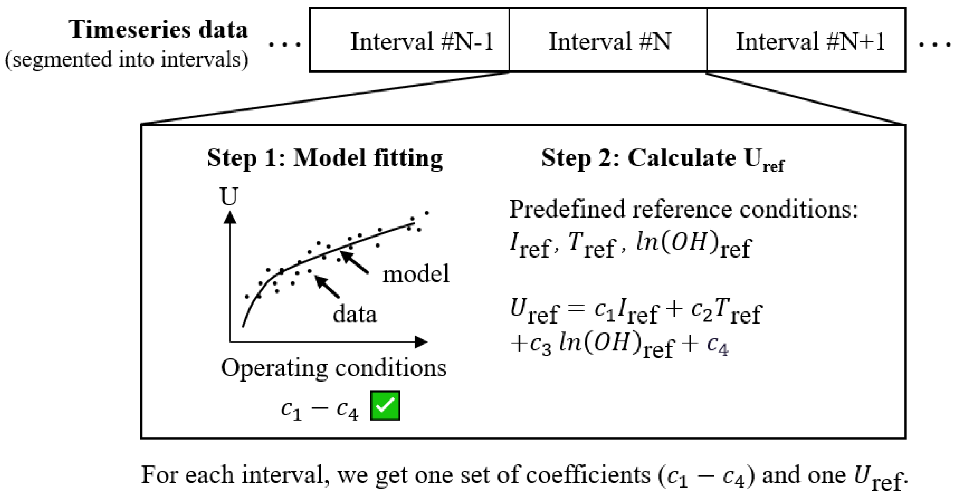
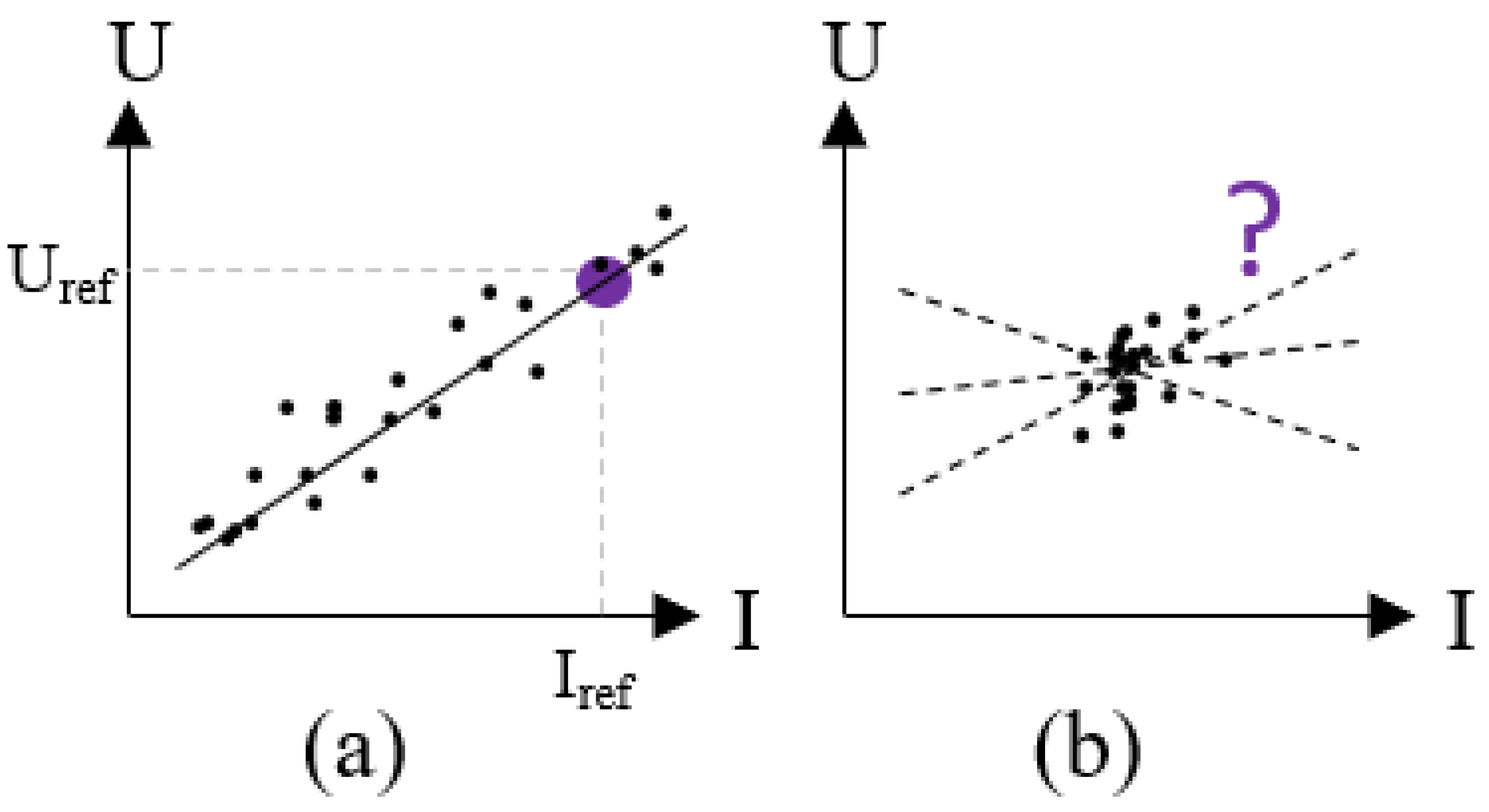
To overcome the limitations of such experiment-based approaches, we propose a data-driven degradation estimation method that corrects the measured voltage to the reference condition (). This is achieved by first building a model that maps the relationship between the voltage and operating conditions, then using the fitted model to calculate the voltage under the reference condition (Figure 1). However, this method faces challenges when the data coverage is limited, as illustrated in Figure 2b. In such cases, the relationship between voltage and operating conditions is ambiguous, causing unstable estimations. (See Section 2 for a detailed problem description).
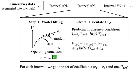
Figure 1.
Calculate the state-of-health indicator from operation data. Step 1: fit a voltage model for each interval. Step 2: use the fitted model to calculate with the predefined reference condition.
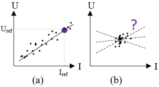
Figure 2.
Case (a): I covers a wide range, then the U-I relation can be well modeled so that can be estimated. Case (b): I varies within a limited range, then the U-I relation is ambiguous, causing uncertain estimation.
The approaches to address the limited data coverage can be broadly classified into data- and model-level approaches. Data-level approaches involve adding new data. This can be achieved by identifying the data gap and then collecting additional data in a targeted manner for the underrepresented group [23]. However, such data collection is only possible if one has control over the data source. Another way to add new data is to generate synthetic data with data augmentation techniques. This has been widely used for image data [24] but is less researched for time-series data [25], especially for multivariate time-series data [26]. Demir et al. [26] proposed using autoencoders, variational autoencoders, and generative adversarial networks (GAN) to augment multivariate time-series data. However, training such neural network-based algorithms on a daily basis—a typical frequency for machine health monitoring—is computationally expensive. Therefore, data augmentation is not a suitable solution for our use case, which is based on multivariate time-series data and requires a daily update.
Model-level approaches use the limited data to train a model without altering the dataset. (For classification problems, this is named few-shot learning [27]). One technique is transfer learning. It transfers a model trained with abundant data from the source domain to the target domain with limited data [28]. Most transfer learning studies are for neural-network-based models [28], which are computationally expensive and not easily explainable. The lack of explainability is a huge barrier for industrial applications due to safety concerns [29]. However, transfer learning for simple, transparent models such as linear regression is much less explored. Chen et al. [30] made a step toward this direction. They developed a data-enriched linear regression algorithm, which built a linear regression model for a small dataset with the help of a large dataset. These two datasets have similar, but not identical, statistical characteristics. This algorithm is the basis for our study and is introduced in detail in Section 3.1. Gross and Tibshirani [31] extended the data-enriched linear regression algorithm to a data shared lasso algorithm, which can build linear regression models simultaneously for multiple datasets. Bouveyron and Jacques [32] introduced a family of transformation models in which the regression coefficients of the target dataset originate from a linear transformation of the coefficients for the source dataset. The most suitable transformation model was selected based on the criteria, including cross-validation error. Dar and Baraniuk [33] focused on over-parameterized linear regression models and analyzed the generalization error with respect to factors such as the number of free parameters. Obst et al. [34] highlighted the fine-tuning technique for transferring a linear regression model and proposed a metric to quantify the benefit of transfer.
This study applies transfer learning to train an empirical linear voltage model over time to provide continuous state-of-health indicators for industrial electrolyzers. Our contributions include
- voltage under the reference condition () as a state-of-health indicator for electrolyzers operated under arbitrary conditions,
- an empirical model for electrolyzer voltage validated with the operation data of industrial electrolyzers,
- a transfer learning algorithm for linear regression models,
- iterative application of the algorithm to time-series data for continuous state-of-health estimation for industrial electrolyzers.
The remainder of this paper is organized as follows. Section 2 introduces the empirical voltage model used in this study and demonstrates the difficulty in model fitting with limited data coverage. Section 3 presents the proposed transfer linear regression algorithm to address the problem of limited data coverage. Section 4 evaluates the proposed algorithm using synthetic and actual industrial operation data. Section 5 discusses the validity of the voltage model and the potential of including prior degradation knowledge from other electrolyzers. Section 6 summarizes the contributions and points out future research directions.
2. Problem Description
In this section, we explain in detail the difficulty of state-of-health estimation for industrial electrolyzers under a limited operation range. We first introduce the industrial operation data used for this research (Section 2.1), then, an empirical model for electrolyzer voltage (Section 2.2). In the end, we show that the model coefficients cannot be well identified when the operation range is limited (Section 2.3).
2.1. Operation Data of an Industrial Electrolyzer
The electrolyzer operation data used in this study are from an industrial proton exchange membrane (PEM) multicell electrolyzer stack, with a nominal power above 0.5 MW. It is operated under atmospheric pressure, around 60 °C. The temperature variation during normal operation is within several degrees. It is operated at medium current density, resulting in a linear voltage–current relationship. The operation profile is not standardized but business-driven, which includes periods of volatile and constant operation. The analyzed data cover a duration of 2 years with a 1-min. resolution. The following measurements are used in this study. Due to confidentiality reasons, more detailed technical specifications cannot be provided.
- Voltage: the average of the single-cell voltages of all electrolyzer cells in a stack, measured with sensors attached to the bipolar plate of each cell.
- Current: the direct current (DC) output of the rectifier supplying power to the electrolyzer stack.
- Temperature: the average stack temperature derived from the mean of the inlet and outlet temperature measurements.
This study focuses on voltage as the degradation indicator for electrolyzers, because it is widely used and easily measurable. There are other possible degradation indicators, such as hydrogen production rate, gas purity, and fluoride release rate, but they are either related to voltage degradation or difficult to measure in industrial setups. This limits the choice of degradation indicators. However, if another easily measurable degradation indicator is of interest, our proposed method in Section 3 can still be applied, as long as the indicator can be expressed in a linear form similar to the Equation (1).
2.2. An Empirical Model for Electrolyzer Voltage
As shown in Figure 1, the first step to derive is to fit a voltage model. There are different types of models for electrolyzer voltage, from simple empirical equations describing voltage as a linear function of current [35,36] to physics-based models considering detailed electrical and thermal effects [37,38]. Empirical models often have simple model structures. The disadvantage is that they are only accurate for a certain operating range and electrolyzer design [39]. In contrast, physics-based models have complex model structures based on physical laws. The disadvantage is that the parameters are difficult to determine.
Since this study focuses on industrial electrolyzers, which are typically designed for a specific operation range, it is not necessary to use an intricate physics-based model. Instead, a model that effectively describes the voltage within the typical operation range is sufficient. Therefore, a simple linear empirical voltage model is adopted:
where voltage (U) is a linear function of current (I), temperature (T), and the natural logarithm of operating hours since the last start (). – are unknown coefficients that need to be fitted for each interval (Step 1 in Figure 1).
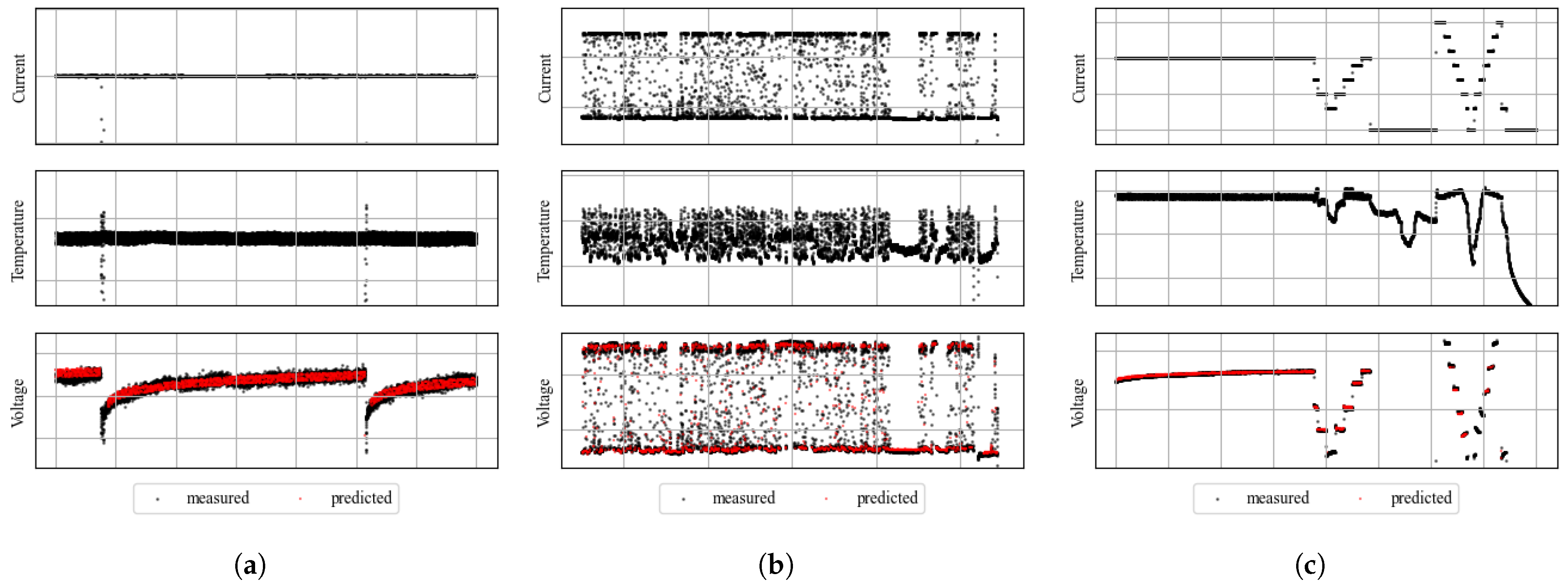
This model is developed by analyzing the operation data of an industrial electrolyzer (Section 2.1). We examined multiple operation intervals with different characteristics. Three examples are shown in Figure 3: (a) constant operation with several starts, (b) volatile operation, and (c) a mixture of constant operation, volatile operation, and starts. The examined intervals have a duration of several days. The operation data are resampled to a 1-min. resolution. The data beyond the normal operation range (e.g., data during standstill, data with extremely low or high current) are excluded. The proposed empirical model (1) is tested on each examined interval; it is trained with 75% of the data and evaluated on the remaining 25% of the data. The results show that the model can accurately describe the voltage with mean squared errors (MSE) at magnitudes of or . Further discussion on the validity of this model can be found in Section 5.1.
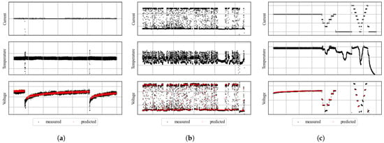
Figure 3.
Model electrolyzer voltage with Equation (1) for three exemplary intervals with different operation characteristics. For confidentiality reasons, the scales are hidden. (a) Interval with constant current input and several starts. MSE: . (b) Interval with strongly volatile operation. MSE: . (c) Interval with a mixture of constant operation, moderately volatile operation, and starts. MSE: .
The unknown coefficients – need to be fitted for each interval (Step 1 in Figure 1). After that, we can calculate the voltage under the predefined reference operating condition (Step 2 in Figure 1) with
where the subscript “ref” denotes the reference condition. The can then be used as a state-of-health indicator for electrolyzers because the influence of the operating conditions on the voltage is removed by statistically correcting the measured voltage to the reference condition.
2.3. Limited Operation Range
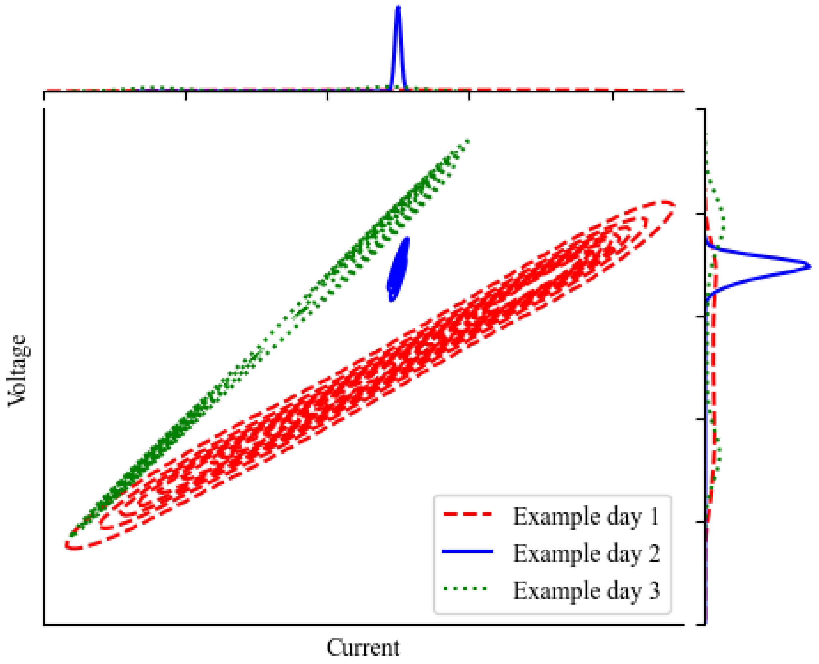
Now we examine the distribution of the actual operation data. Figure 4 shows the voltage–current distribution of three 24-hour intervals. First, it is observed that the slope changes, which is clear evidence of degradation. This requires the model (1) to be updated regularly to capture the change. In addition, the data spread is different. This is a major difference between industrial operations and laboratory experiments. Industrial electrolyzers are controlled by the operator based on their business needs, without a predefined pattern. Any operation pattern, such as with constant current input (example day 2) or with varying current input (example day 1 and 3), could occur. Time intervals similar to example day 2, in which the operation range is very limited, can make model fitting cumbersome, as illustrated in Figure 2b. This problem applies to all the right-hand-side variables I, T, and in the model (1).

Figure 4.
Voltage–current distribution of three example days. Voltage is a function of several variables. To simplify the visualization, only the electric current is plotted on the x-axis here.
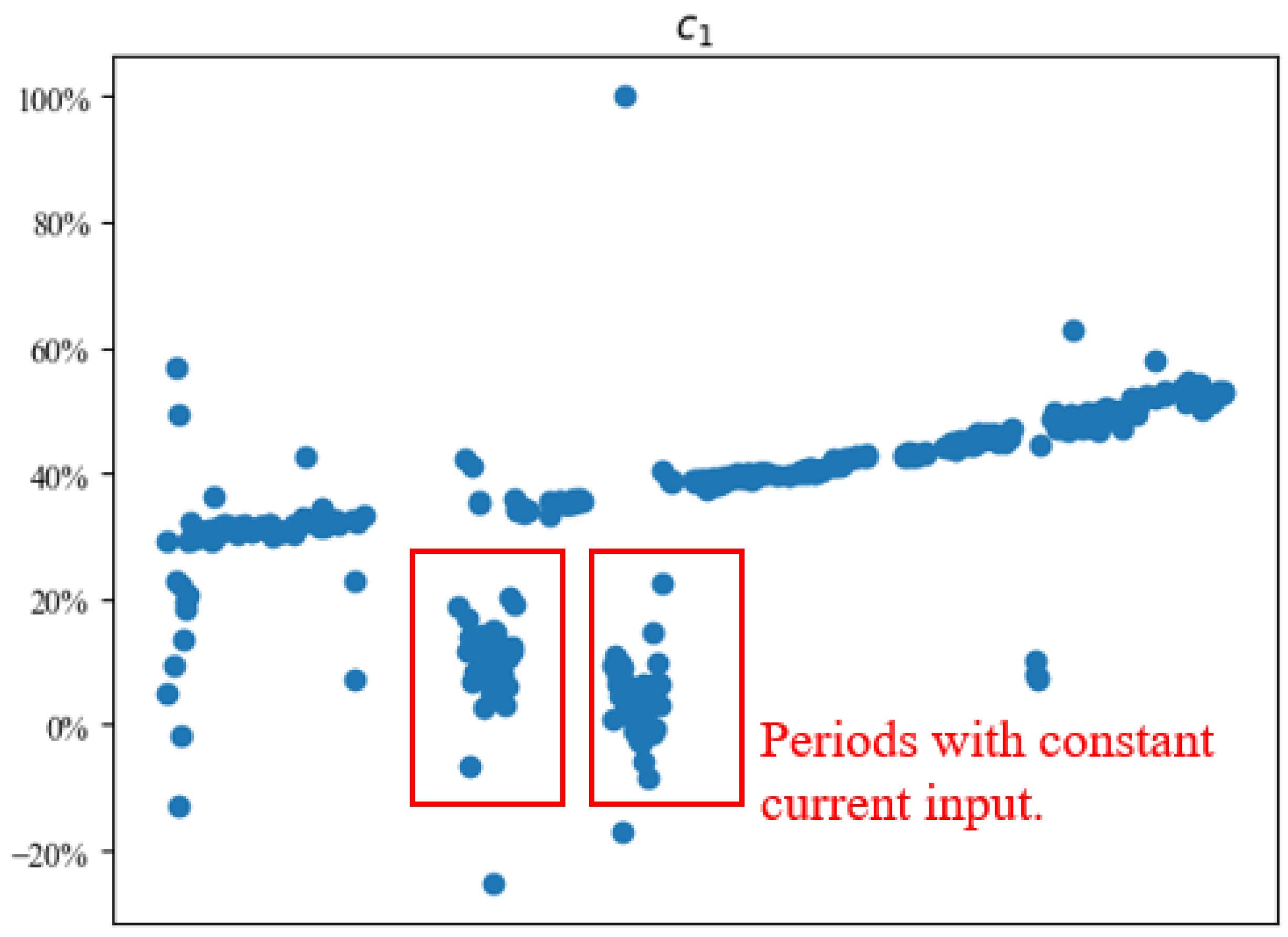
To further demonstrate the problem of the limited operation range, we fit the model (1) on each day independently without applying any transfer learning technique. Figure 5 shows that the fitted coefficient increases in general, which aligns with our physical understanding of degradation, but the coefficient at periods with constant current input (similar to example day 2 in Figure 4) cannot be easily identified due to the limited data coverage.
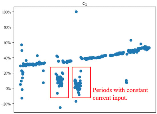
Figure 5.
The linear coefficient for current () cannot be well estimated during constant operation periods. For confidentiality reasons, the coefficient is shown on a percentage scale.
As mentioned in Section 1, transfer learning can mitigate the problem of limited data coverage. In the next section, we introduce the transfer linear regression algorithm that uses a fitted voltage model to assist the model fitting process.
3. Method
The transfer linear regression (TLR) algorithm is inspired by the data-enriched linear regression algorithm proposed in [30]. This is introduced first as the foundation for the TLR algorithm.
3.1. Data-Enriched Linear Regression
The data-enriched linear regression algorithm was proposed by Chen et al. in 2015 [30]. It aims to build a linear regression model for a small dataset with the help of a second large, but possibly biased, dataset. This use case is very similar to ours, as our main purpose is to build a model for intervals with a limited operation range (the small dataset) with the help of historical data that cover a larger operation range but have another degradation state (the second large but biased dataset), and our base model (1) also has a linear form.
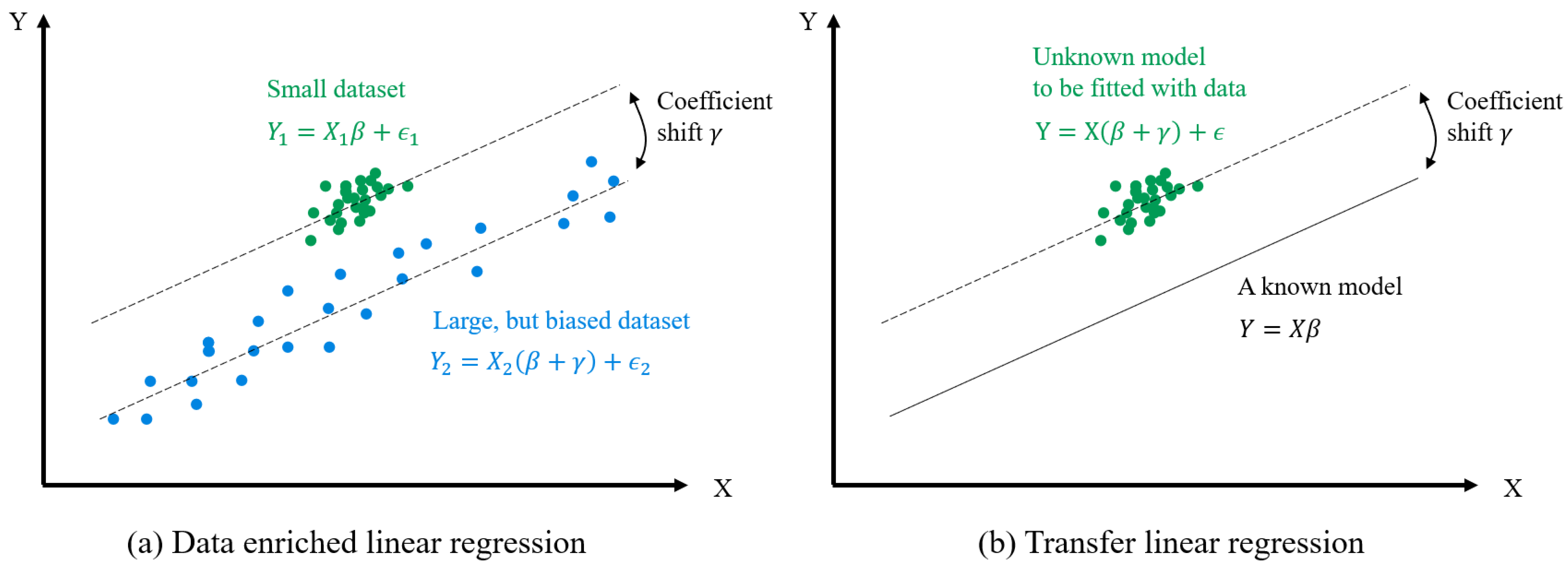
As illustrated in Figure 6a, the data-enriched linear regression algorithm assumes that the small dataset follows a linear regression model
where and are the independent and dependent variables, is the linear coefficient, and is the error. The second dataset follows the model
where and are the independent and dependent variables, is the error, and the linear coefficients are shifted by . The parameter corresponds to the drift and rotation of the model.

Figure 6.
Illustration for (a) data-enriched linear regression algorithm and (b) transfer linear regression algorithm.
The parameters and are estimated by minimizing the loss function
The first two terms in the loss function are the squared errors of (3) and (4). This is similar to the ordinary least squares regression technique, which estimates model coefficients by minimizing the fitting error. The third term controls the coefficient drift . The reason for controlling is to restrict the shape of the model (Figure 6a). Without this controlling term, the model is unstable when the data coverage is limited (Figure 2b).
Two hyperparameters and are required to control . controls the overall size of . To provide some further understanding: setting means no constraint on ; therefore, and are fitted separately with the two datasets; in contrast, setting forces , which is equivalent to fitting with two datasets jointly. The second hyperparameter can be used to control each value in the vector in detail, but the paper [30] does not provide concrete instructions on how to construct the matrix.
As a result, the estimated parameters and , by minimizing the loss function (5), are
where and [30].
3.2. Transfer Linear Regression
3.2.1. Mathematical Formulation
The TLR algorithm is a modification of the data-enriched linear regression algorithm (Figure 6b). The difference is that the data-enriched linear regression algorithm uses two datasets to estimate two parameters and , whereas the TLR algorithm uses only one dataset to estimate , assuming that the parameter is already known (e.g., fitted with historical data or derived from expert knowledge). This setup enables the inclusion of an existing model without requiring a second database and is computationally cheaper by handling smaller data matrices.
The TLR algorithm aims to estimate the parameter in the equation
where X and Y are the data from the target dataset, and is already known. Analogous to the data-enriched linear regression algorithm, the unknown parameter can be estimated by minimizing the loss function
This gives
The derivation process is detailed in Appendix A. The hyperparameters and control the size of in the same manner as the data-enriched linear regression. Their impacts are further detailed in Section 3.2.4.
In summary, the TLR algorithm is proposed for state-of-health estimation because
- it can capture the model drift caused by degradation,
- it tackles the problem of limited data coverage due to constant operation,
- it is suitable for a linear model,
- it is computationally efficient by not including a second dataset,
- and its model transfer mechanism is easy to interpret.
3.2.2. Application on Time-Series Data
To realize continuous state-of-health estimation along the lifetime of electrolyzers, we propose an iterative model fitting process that continuously updates a linear regression model along a time series. Algorithm 1 shows a minimum example of a time-series application. Several modifications can be implemented in practice. For example, one can set and/or flexibly for each interval instead of fixing a global value for all intervals; one can also add a fitting quality check for each interval—if the fitting accuracy is not satisfactory, one can use instead of (i.e., not updating the coefficients). Section 4 presents the detailed procedure for the evaluation cases.
| Algorithm 1 Apply TLR on time-series data |
| Input: Initial coefficients , hyperparameters and , time series data X and Y segmented into n intervals (, ), … (, ) |
| Output: Coefficients for all n intervals , … |
| for to n do |
| end for |
3.2.3. Setting Initial Coefficients
Algorithm 1 requires an initial coefficient . There are different methods to obtain : it can be derived from the initial time-series data, data from other similar systems, or expert knowledge. For the evaluation cases in this study (Section 4), is derived from the initial (first 10%) time-series data.
3.2.4. Impacts of Hyperparameters and
Hyperparameters and need to be set before model fitting. Same as in the data-enriched linear regression algorithm [30], is a constant that controls the overall size of . Its impact can be seen from the following examples of setting extreme values for (also summarized in Table 1):

Table 1.
Impacts of setting extreme values for hyperparameters and .
- Setting forces . This leads to ; that is, the linear coefficients do not change over time; therefore, we expect high fitting errors along the time series.
- In contrast, setting implies no constraint on the size of . Equation (9) becomesthat is, is estimated freely by minimizing the fitting error. The freedom of leads to the freedom of (11), meaning that is not influenced by the previous coefficient . This is equivalent to independent fitting for each interval. In this case, we expect fluctuating and low fitting errors along the time series.
Regarding , the original paper on data-enriched linear regression [30] does not provide concrete instructions on how to construct . For TLR, we define as a diagonal matrix with dimensions (p is the dimension of and ):
The term in (6) and (9) is then
This shows that the diagonal elements can control the individual values in the vector separately. The impact of the diagonal elements is similar to that of (Table 1).
Table 1 summarizes the impacts of setting extreme values for and . It shows that setting small values for and results in a low fitting error but fluctuating coefficients, whereas setting high values has the opposite impact. Balancing the trade-off between the fitting accuracy and coefficient stability is key to setting proper values for and . This is introduced in the following subsections.
3.2.5. Setting
As explained above, setting involves a trade-off between the fitting accuracy and coefficient stability. In practice, we can test different s on multiple intervals and choose a suitable value by observing the coefficient distribution and fitting accuracy. This is demonstrated in Section 4.
3.2.6. Setting Diagonal Elements in
Recall that is a diagonal matrix, and p is the dimension of and , namely, the number of variables. Table 1 shows that for any variable p, setting leads to , i.e., the linear coefficient stays constant along the time series; whereas setting leads to flexible . That means, if the coefficient for variable p is allowed to have a large variation, the corresponding should be small. Large variations should be allowed when
- (a) the coefficient varies largely by nature over time.
- (b) the variable p covers a wide range during an interval. (In this case, can be easily identified because of the wide data coverage, so we allow it to be fitted flexibly with the data. On the contrary, if the variable p covers only a small range in interval i, such as in example day 2 in Figure 4, we fix toward ).
Applying these principles in the electrolyzer context, we design the matrix as in Algorithm 2. The calculations can also be customized for other use cases.
| Algorithm 2 Setting diagonal elements in for electrolyzers |
|
4. Evaluation
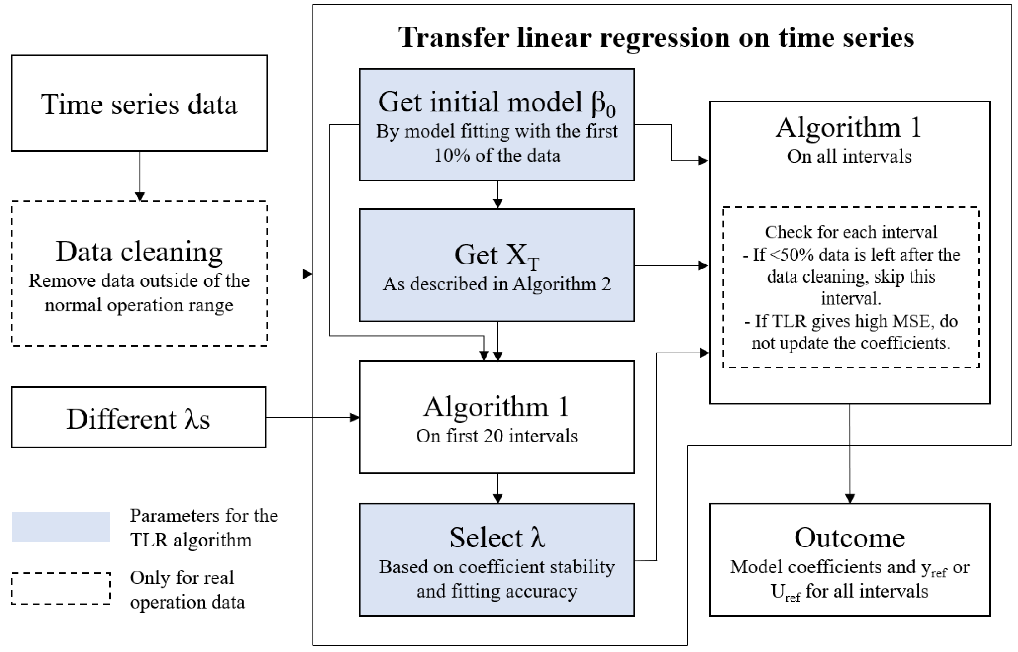
The TLR algorithm is evaluated in two settings: (1) with synthetic data (Section 4.1), where the ground truth is known, and (2) with real operation data from industrial electrolyzers (Section 4.2), where the ground truth (measured ) is sparsely known due to volatile operation. In both settings, the TLR algorithm is compared with plain linear regression (PLR), to highlight the necessity and effectiveness of transfer learning. The TLR algorithm is executed as shown in Figure 7.
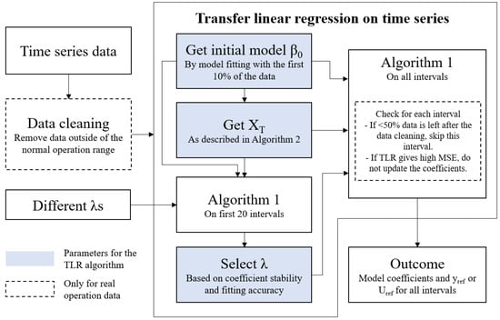
Figure 7.
The execution process of the TLR algorithm. The dashed boxes are only for the evaluation case with real operation data (Section 4.2).
4.1. Method Validation with Synthetic Data
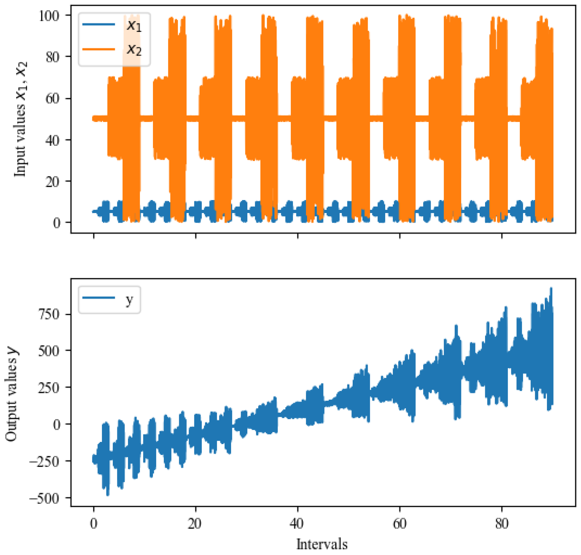
The synthetic data are generated using the model . The coefficient grows linearly from −50 to 50, grows linearly from 0 to 5, and remains constant at 5. We simulate 90 intervals, with 100 data points per interval. Each interval has different variation levels for and . varies between 0 and 10 at high variation intervals, 3 and 7 at middle variation intervals, or 4.9 and 5.1 at low variation intervals. varies between 0 and 100 at high variation intervals, 30 and 70 at middle variation intervals, or 49 and 51 at low variation intervals. The noise is random within . The reference condition is set at and , so y under the reference condition is calculated with . The synthetic data are shown in Figure 8.
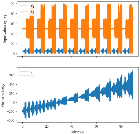
Figure 8.
Synthetic data for 90 intervals with various data coverage.
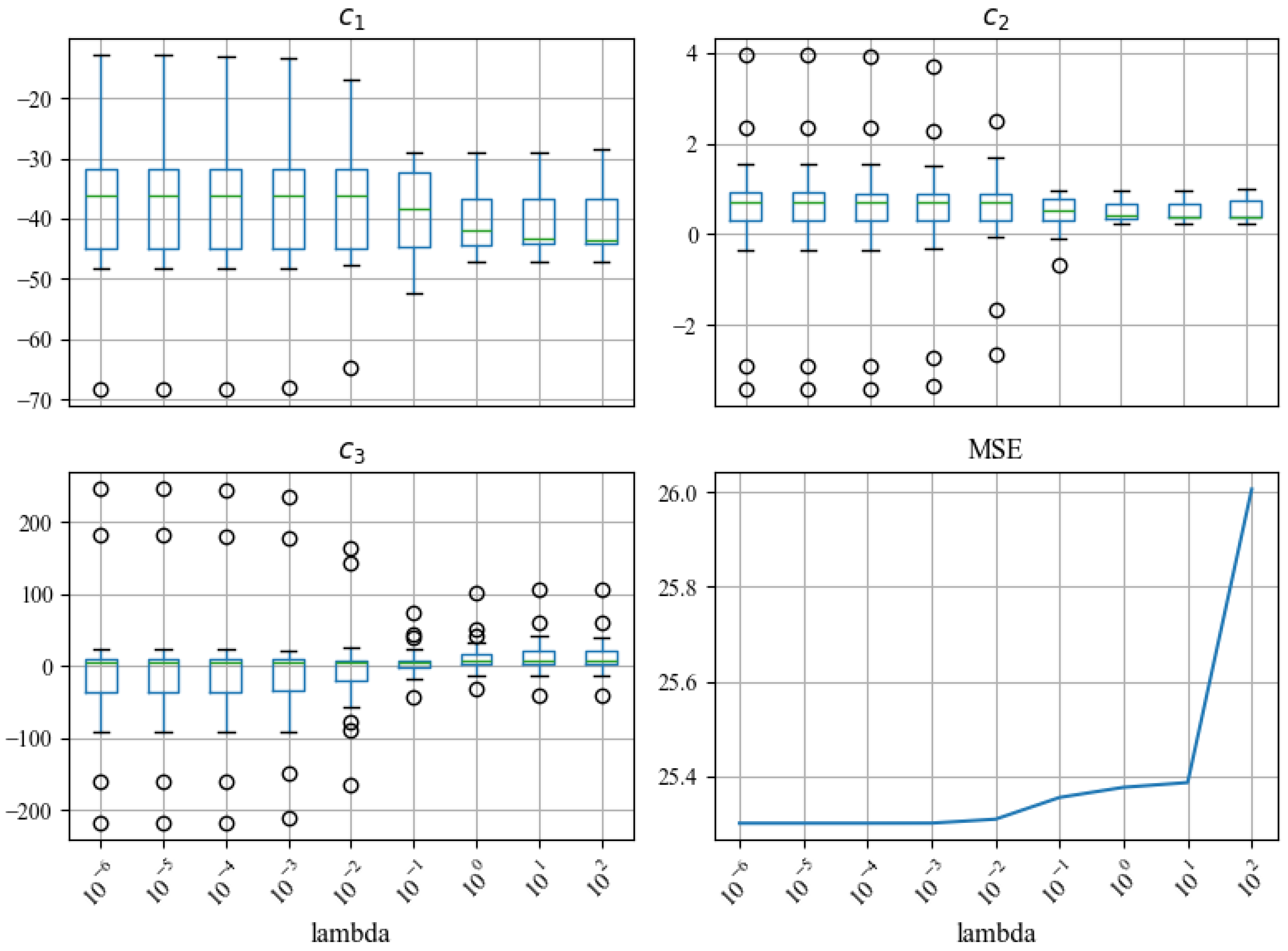
As described in Section 3.2.5, we test 9 different values from to (Figure 9). This range allows us to observe the changes in the coefficient stability and fitting error; as increases, the coefficients become more stable (the heights of the box plots become shorter) and MSE increases, which aligns with our expectations in Table 1. We select as a trade-off between coefficient stability and model accuracy.
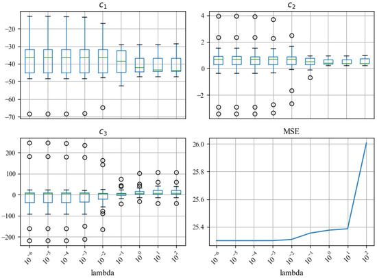
Figure 9.
Different s ranging from to are tested. As increases, the coefficients – become more stable (the spreads of the box plots become smaller), and fitting error MSE increases, which aligns with Table 1.
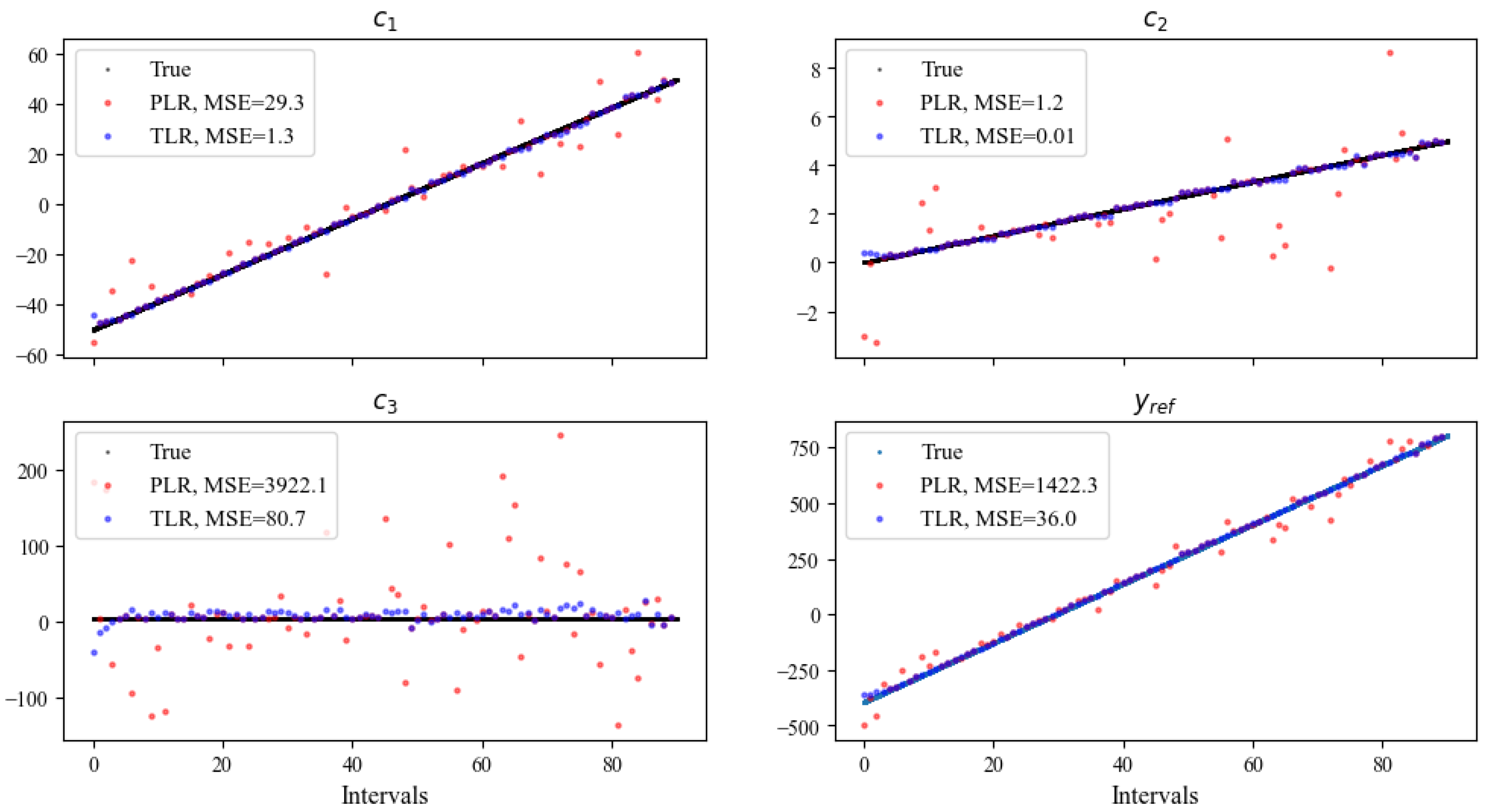
Using the selected , we run the transfer linear regression process (Algorithm 1) and compare the results with PLR (Figure 10). The comparison shows that the TLR algorithm can capture the true coefficients and with significantly smaller errors than PLR. This demonstrates the effectiveness of the transfer learning technique.
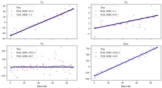
Figure 10.
TLR can capture the ground truth with significantly smaller errors than PLR.
The full process of model validation with synthetic data is available in the Jupyter Notebook in the Supplementary Material.
4.2. Method Validation with Industrial Operation Data
Now we apply the transfer linear regression algorithm to the actual operation data of an industrial electrolyzer (Section 2.1). We first fit the empirical voltage model (1) with the TLR algorithm (Algorithm 1) for each day and then use the fitted model to calculate the state-of-health indicator (2).
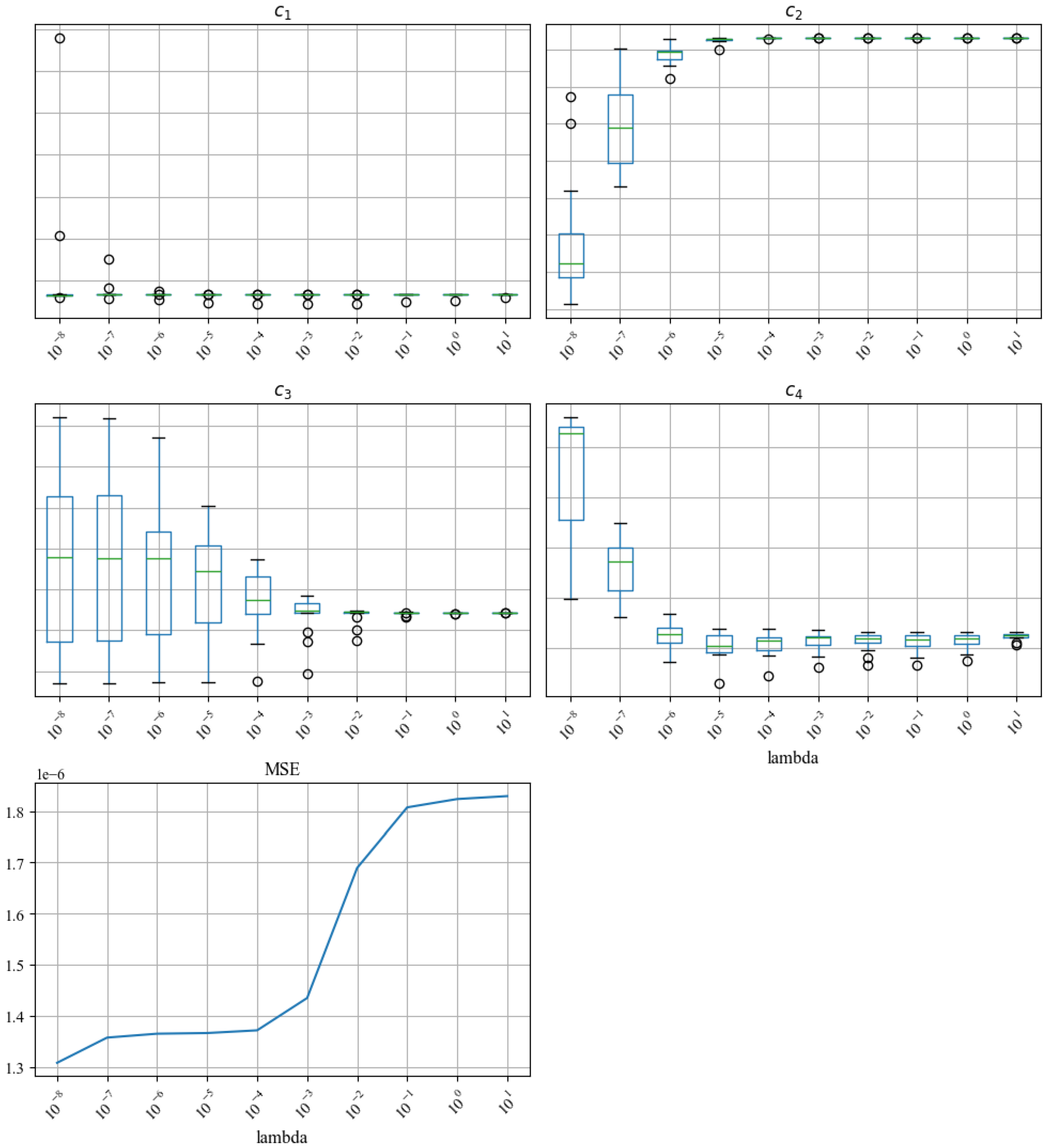
To execute the TLR algorithm (Algorithm 1), the hyperparameter needs to be selected. As described in Section 3.2.5, we test 10 different values from to 10 (Figure 11). This range allows us to observe the changes in the coefficient stability and fitting error; as increases, the coefficients become more stable (the heights of the box plots become shorter) and MSE increases, which aligns with our expectations in Table 1. We select as a trade-off between coefficient stability and model accuracy.
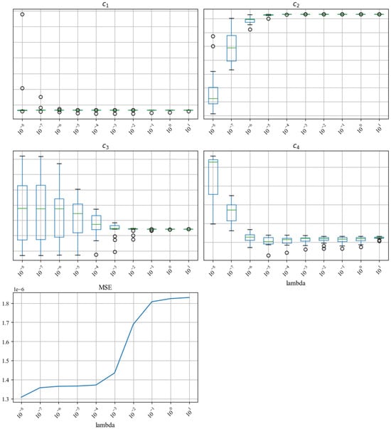
Figure 11.
Different s ranging from to 10 are tested. As increases, the coefficients – become more stable (the spreads of the box plots become smaller), and the fitting error MSE increases, which aligns with Table 1. For confidentiality reasons, the y-axis scales for the coefficients are hidden.
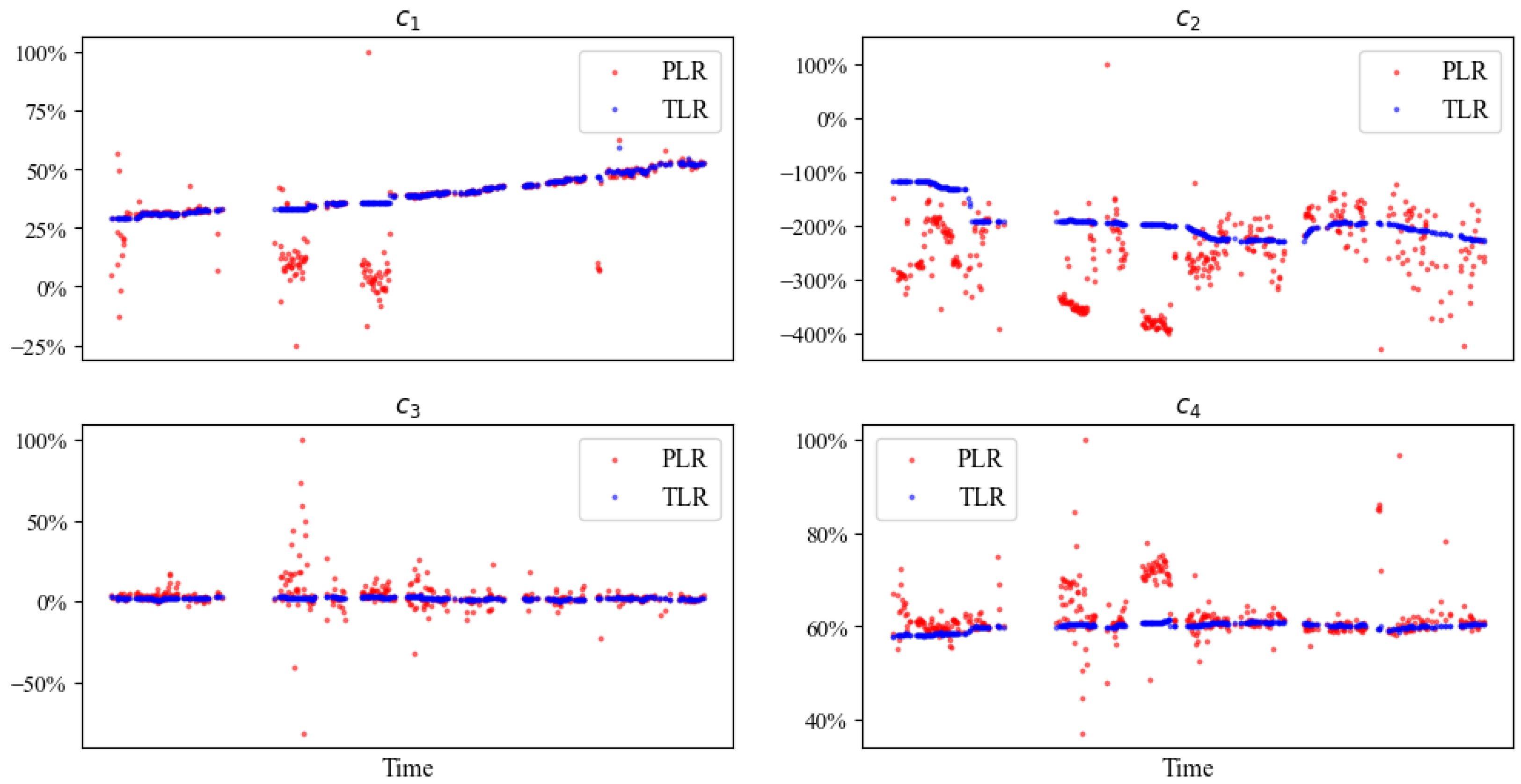
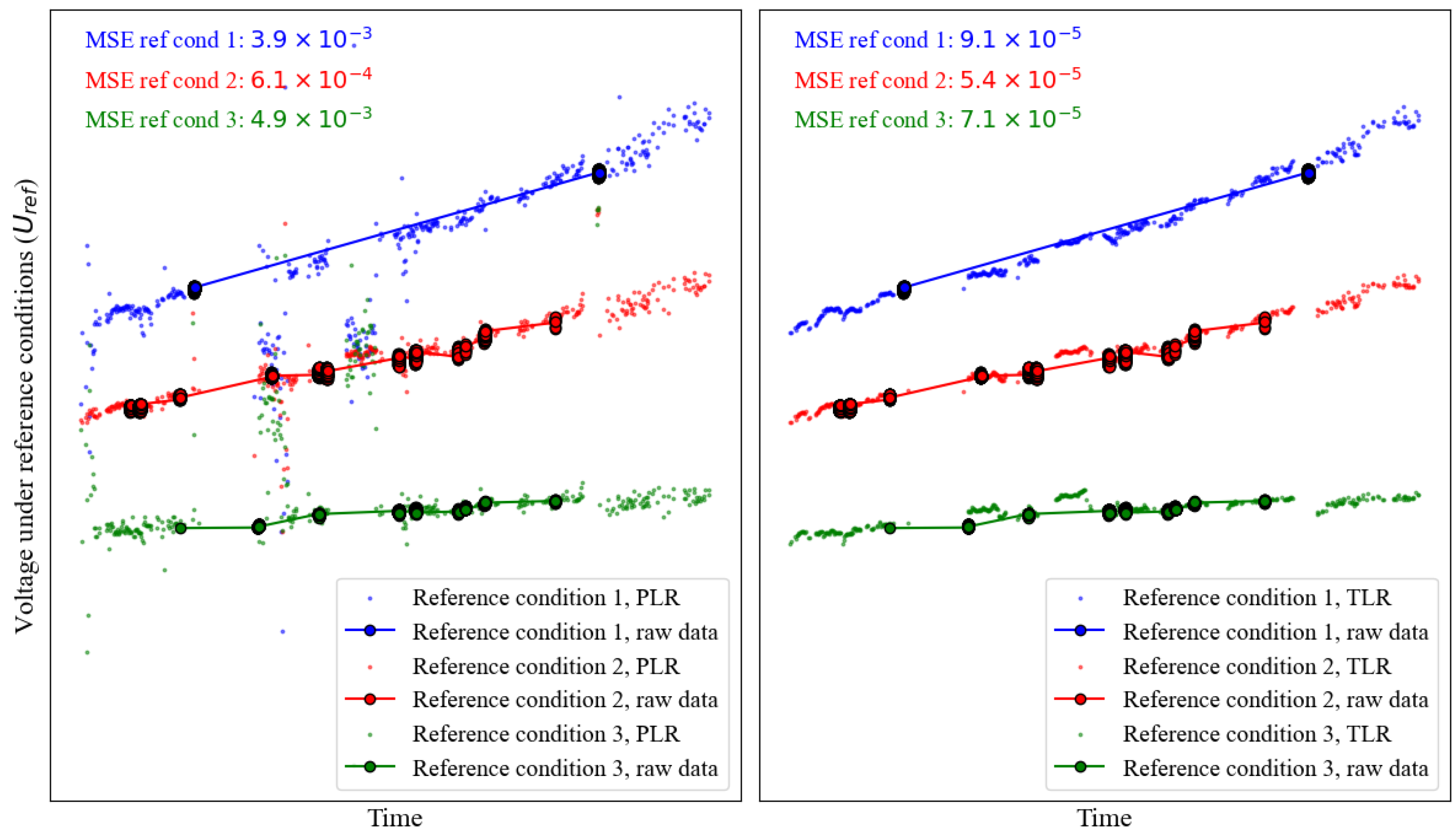
Using the selected , we run the TLR process (Algorithm 1) and compare the results with PLR. Figure 12 shows that PLR produces unstable coefficients, which contradicts the gradual degradation process. This further leads to a fluctuating and inaccurate calculation in Figure 13 (left). In contrast, the coefficients estimated with TLR evolve much more smoothly (Figure 12), and the calculated state-of-health indicator is also more stable and accurate (Figure 13, right). This shows the necessity and effectiveness of the transfer learning technique in handling actual industrial operation data.
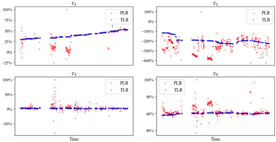
Figure 12.
Coefficients fitted with the TLR algorithm evolve smoothly with much less fluctuation than with PLR. For confidentiality reasons, the coefficients are shown in percentage scale.
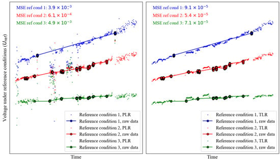
Figure 13.
calculated with PLR process (left) and TLR process (right) under 3 different reference conditions. They are compared with the raw data filtered at the reference conditions. Note that the raw data are only sparsely available because the operating conditions are volatile and rarely at the reference condition. This is the motivation to derive the health indicator for continuous condition monitoring. In addition to its sparsity, the raw data also have a different time resolution than the calculated . Therefore, for calculating MSE, data are first resampled to the same time resolution and gaps are filled with linear interpolation. For confidentiality reasons, the axes scales are hidden.
In addition to the methodological comparison between TLR and PLR, we also evaluate the quality of derived from TLR against the quality of the actual measurement. Specifically, the error magnitude in should not exceed that in the actual measurement. The measurement error of the voltage sensor is below 0.01 V, which translates to a squared error of . The MSE of computed with TLR (Figure 13, right) is consistently below this threshold. This signifies that the overall quality of is satisfactory and within acceptable bounds.
5. Discussion
5.1. Validity of the Empirical Voltage Model
In this study, we use the empirical voltage model (1) to map the relationship between voltage and operating conditions. Its simple linear structure ensures rapid computation and still provides good accuracy for the studied industrial electrolyzers (Figure 3). However, due to the nature of an empirical model, its accuracy cannot be guaranteed for other electrolyzer designs or other operation schemes. For example, model (1) implies a linear relationship between U and I. This is valid for electrolyzers operated at medium current density, where the ohmic overpotential dominates, resulting in a linear U-I-relation; whereas for electrolyzers operated at low current density, where the non-linear activation overpotential dominates, the non-linear U-I-relation must be considered in the voltage model. Therefore, the accuracy of this model needs to be checked when it is applied to other electrolyzer systems. If the accuracy is insufficient, the model needs to be adapted.
5.2. Use Prior Degradation Knowledge to Assist Model Fitting
Although the evaluation cases in Section 4 demonstrate the capability of TLR in model estimation for varying data coverages, it should be applied with caution if an electrolyzer is under constant operation for a long period: if a variable has a small coverage in an interval due to constant operation, the coefficient for this variable tends to be the same as in the last interval. If such constant operation lasts continuously over a long period, the coefficient fitted with the TLR process drifts from the true value. To overcome this limitation, one can try to include prior knowledge (e.g., from the degradation history of similar electrolyzers) in the fitting process. Prior knowledge can provide additional information that helps to update the model coefficients even under extensively long periods of constant operation.
6. Conclusions
Tracking the degradation states of electrolyzers is essential for economical and safe operation. One of the direct consequences of degradation is the increase in voltage. However, due to the impact of operation conditions, the measured voltage cannot be directly used as a degradation indicator. The existing approaches to measure degradation (such as polarization curve tests) require strict control of the operating conditions, and thus, are impractical for industrial application. To solve this problem, we propose a data-driven degradation estimation method suitable for industrial electrolyzers operated under arbitrary conditions.
The key to this method is to convert the measured voltage under arbitrary operating conditions to a reference condition—. The calculation of consists of two steps: (1) fitting a voltage model for each interval and (2) using the fitted model and predefined reference conditions to calculate . An empirical voltage model is used, which is developed based on the operation data of industrial electrolyzers and can accurately model the voltage with an MSE at a magnitude of . The model fitting step can be challenging with a limited operation range. To address this problem, we propose the TLR algorithm, which transfers a pre-existing model to the target interval. The essence of TLR is to constrain the change in the model coefficients, enabling stable estimation of these coefficients even in intervals with a limited operation range.
The TLR algorithm is first validated with synthetic data, showing that the algorithm can capture the ground truth with significantly lower errors than plain linear regression. The TLR algorithm is also applied to 2 years of actual operation data from an industrial electrolyzer. The results show that the TLR algorithm can smoothly estimate the coefficients of the voltage model and provide stable values.
Further research could focus on integrating prior knowledge into the fitting process. The prior knowledge can be derived from the degradation history of similar electrolyzers. By integrating prior knowledge, the model fitting relies not only on the fitted model from the last interval of the same electrolyzer but also on the long-term degradation experience of multiple electrolyzers. Further research might also explore various empirical models to attain a more universally applicable yet simple model.
Supplementary Materials
The following supporting information can be downloaded at: https://www.mdpi.com/article/10.3390/en17061374/s1, Jupyter Notebook for method validation with synthetic data (Section 4.1).
Author Contributions
Conceptualization, methodology, validation, and formal analysis, X.Y.; writing—original draft preparation, X.Y. and C.L.; writing—review and editing and supervision, F.H. and A.N. All authors have read and agreed to the published version of the manuscript.
Funding
This research was funded by the Federal Ministry of Education and Research of Germany under the projects SEGIWA (grant number: 03HY121A) and DERIEL (grant number: 03HY122A).
Data Availability Statement
The synthetic data can be reproduced with the Jupyter Notebook provided in the Supplementary Material. The industrial operation data are not readily available due to the data confidentiality contract with the industrial partner.
Conflicts of Interest
The authors declare no conflicts of interest.
Abbreviations
The following abbreviations are used in this manuscript:
| DC | Direct current |
| MSE | Mean squared error |
| PEM | Proton exchange membrane |
| PLR | Plain linear regression |
| TLR | Transfer linear regression |
References
- Smolinka, T.; Ojong, E.T.; Lickert, T. Fundamentals of PEM water electrolysis. In PEM Electrolysis for Hydrogen Production; CRC Press: Boca Raton, FL, USA, 2015; pp. 11–33. [Google Scholar]
- Rizwan, M.; Alstad, V.; Jäschke, J. Design considerations for industrial water electrolyzer plants. Int. J. Hydrogen Energy 2021, 46, 37120–37136. [Google Scholar] [CrossRef]
- Xue, B.; Xu, H.; Huang, X.; Zhu, K.; Xu, Z.; Pei, H. Similarity-based prediction method for machinery remaining useful life: A review. Int. J. Adv. Manuf. Technol. 2022, 121, 1501–1531. [Google Scholar] [CrossRef]
- Zhang, Y.; Wik, T.; Bergström, J.; Pecht, M.; Zou, C. A machine learning-based framework for online prediction of battery ageing trajectory and lifetime using histogram data. J. Power Sources 2022, 526, 231110. [Google Scholar] [CrossRef]
- Severson, K.A.; Attia, P.M.; Jin, N.; Perkins, N.; Jiang, B.; Yang, Z.; Chen, M.H.; Aykol, M.; Herring, P.K.; Fraggedakis, D.; et al. Data-driven prediction of battery cycle life before capacity degradation. Nat. Energy 2019, 4, 383–391. [Google Scholar] [CrossRef]
- Shu, X.; Shen, J.; Li, G.; Zhang, Y.; Chen, Z.; Liu, Y. A flexible state-of-health prediction scheme for lithium-ion battery packs with long short-term memory network and transfer learning. IEEE Trans. Transp. Electrif. 2021, 7, 2238–2248. [Google Scholar] [CrossRef]
- Che, Y.; Deng, Z.; Lin, X.; Hu, L.; Hu, X. Predictive battery health management with transfer learning and online model correction. IEEE Trans. Veh. Technol. 2021, 70, 1269–1277. [Google Scholar] [CrossRef]
- Sønderskov, S.H.; Ilsøe, J.W.; Rasmussen, D.; Blom-Hansen, D.; Munk-Nielsen, S. State of Health Estimation and Prediction of Fuel Cell Stacks in Backup Power Systems. engrXiv 2019. [Google Scholar] [CrossRef]
- Zhang, D.; Baraldi, P.; Cadet, C.; Yousfi-Steiner, N.; Bérenguer, C.; Zio, E. An ensemble of models for integrating dependent sources of information for the prognosis of the remaining useful life of Proton Exchange Membrane Fuel Cells. Mech. Syst. Signal Process. 2019, 124, 479–501. [Google Scholar] [CrossRef]
- Olsson, T.; Ramentol, E.; Rahman, M.; Oostveen, M.; Kyprianidis, K. A data-driven approach for predicting long-term degradation of a fleet of micro gas turbines. Energy AI 2021, 4, 100064. [Google Scholar] [CrossRef]
- Mao, W.; He, J.; Sun, B.; Wang, L. Prediction of bearings remaining useful life across working conditions based on transfer learning and time series clustering. IEEE Access 2021, 9, 135285–135303. [Google Scholar] [CrossRef]
- Zhao, H.; Liu, H.; Jin, Y.; Dang, X.; Deng, W. Feature extraction for data-driven remaining useful life prediction of rolling bearings. IEEE Trans. Instrum. Meas. 2021, 70, 1–10. [Google Scholar] [CrossRef]
- Yang, X.; Fang, Z.; Li, X.; Yang, Y.; Mba, D. Similarity-based information fusion grey model for remaining useful life prediction of aircraft engines. Grey Syst. Theory Appl. 2021, 11, 463–483. [Google Scholar] [CrossRef]
- Huang, C.G.; Huang, H.Z.; Peng, W.; Huang, T. Improved trajectory similarity-based approach for turbofan engine prognostics. J. Mech. Sci. Technol. 2019, 33, 4877–4890. [Google Scholar] [CrossRef]
- Liu, Y.; Hu, X.; Zhang, W. Remaining useful life prediction based on health index similarity. Reliab. Eng. Syst. Saf. 2019, 185, 502–510. [Google Scholar] [CrossRef]
- Wang, H.; Ni, G.; Chen, J.; Qu, J. Research on rolling bearing state health monitoring and life prediction based on PCA and Internet of things with multi-sensor. Measurement 2020, 157, 107657. [Google Scholar] [CrossRef]
- Yu, W.; Kim, I.Y.; Mechefske, C. Remaining useful life estimation using a bidirectional recurrent neural network based autoencoder scheme. Mech. Syst. Signal Process. 2019, 129, 764–780. [Google Scholar] [CrossRef]
- Yu, W.; Kim, I.Y.; Mechefske, C. Analysis of different RNN autoencoder variants for time series classification and machine prognostics. Mech. Syst. Signal Process. 2021, 149, 107322. [Google Scholar] [CrossRef]
- Tsotridis, G.; Pilenga, A. EU Harmonised Protocols for Testing of Low Temperature Water Electrolysers; European Comission: Brussels, Belgium, 2021. [Google Scholar]
- Li, N.; Araya, S.S.; Kær, S.K. Long-term contamination effect of iron ions on cell performance degradation of proton exchange membrane water electrolyser. J. Power Sources 2019, 434, 226755. [Google Scholar] [CrossRef]
- Weiß, A.; Siebel, A.; Bernt, M.; Shen, T.H.; Tileli, V.; Gasteiger, H. Impact of intermittent operation on lifetime and performance of a PEM water electrolyzer. J. Electrochem. Soc. 2019, 166, F487. [Google Scholar] [CrossRef]
- Suermann, M.; Bensmann, B.; Hanke-Rauschenbach, R. Degradation of proton exchange membrane (PEM) water electrolysis cells: Looking beyond the cell voltage increase. J. Electrochem. Soc. 2019, 166, F645. [Google Scholar] [CrossRef]
- Asudeh, A.; Jin, Z.; Jagadish, H. Assessing and remedying coverage for a given dataset. In Proceedings of the 2019 IEEE 35th International Conference on Data Engineering (ICDE), Macao, China, 8–11 April 2019; pp. 554–565. [Google Scholar]
- Shorten, C.; Khoshgoftaar, T.M. A survey on image data augmentation for deep learning. J. Big Data 2019, 6, 1–48. [Google Scholar] [CrossRef]
- Wen, Q.; Sun, L.; Yang, F.; Song, X.; Gao, J.; Wang, X.; Xu, H. Time series data augmentation for deep learning: A survey. arXiv 2020, arXiv:2002.12478. [Google Scholar]
- Demir, S.; Mincev, K.; Kok, K.; Paterakis, N.G. Data augmentation for time series regression: Applying transformations, autoencoders and adversarial networks to electricity price forecasting. Appl. Energy 2021, 304, 117695. [Google Scholar] [CrossRef]
- Wang, Y.; Yao, Q.; Kwok, J.T.; Ni, L.M. Generalizing from a few examples: A survey on few-shot learning. ACM Comput. Surv. 2020, 53, 1–34. [Google Scholar] [CrossRef]
- Weiss, K.; Khoshgoftaar, T.M.; Wang, D. A survey of transfer learning. J. Big Data 2016, 3, 1–40. [Google Scholar] [CrossRef]
- Guidotti, R.; Monreale, A.; Ruggieri, S.; Turini, F.; Giannotti, F.; Pedreschi, D. A survey of methods for explaining black box models. ACM Comput. Surv. 2018, 51, 1–42. [Google Scholar] [CrossRef]
- Chen, A.; Owen, A.B.; Shi, M. Data enriched linear regression. Electron. J. Stat. 2015, 9, 1078–1112. [Google Scholar] [CrossRef]
- Gross, S.M.; Tibshirani, R. Data Shared Lasso: A novel tool to discover uplift. Comput. Stat. Data Anal. 2016, 101, 226–235. [Google Scholar] [CrossRef]
- Bouveyron, C.; Jacques, J. Adaptive linear models for regression: Improving prediction when population has changed. Pattern Recognit. Lett. 2010, 31, 2237–2247. [Google Scholar] [CrossRef][Green Version]
- Dar, Y.; Baraniuk, R.G. Double double descent: On generalization errors in transfer learning between linear regression tasks. SIAM J. Math. Data Sci. 2022, 4, 1447–1472. [Google Scholar] [CrossRef]
- Obst, D.; Ghattas, B.; Cugliari, J.; Oppenheim, G.; Claudel, S.; Goude, Y. Transfer learning for linear regression: A statistical test of gain. arXiv 2021, arXiv:2102.09504. [Google Scholar]
- Atlam, O.; Kolhe, M. Equivalent electrical model for a proton exchange membrane (PEM) electrolyser. Energy Convers. Manag. 2011, 52, 2952–2957. [Google Scholar] [CrossRef]
- Sossan, F.; Bindner, H.; Madsen, H.; Torregrossa, D.; Chamorro, L.R.; Paolone, M. A model predictive control strategy for the space heating of a smart building including cogeneration of a fuel cell-electrolyzer system. Int. J. Electr. Power Energy Syst. 2014, 62, 879–889. [Google Scholar] [CrossRef]
- Abomazid, A.M.; El-Taweel, N.A.; Farag, H.E. Novel analytical approach for parameters identification of PEM electrolyzer. IEEE Trans. Ind. Inform. 2021, 18, 5870–5881. [Google Scholar] [CrossRef]
- Krenz, T.; Weiland, O.; Trinke, P.; Helmers, L.; Eckert, C.; Bensmann, B.; Hanke-Rauschenbach, R. Temperature and Performance Inhomogeneities in PEM Electrolysis Stacks with Industrial Scale Cells. J. Electrochem. Soc. 2023, 170, 044508. [Google Scholar] [CrossRef]
- Falcão, D.; Pinto, A. A review on PEM electrolyzer modelling: Guidelines for beginners. J. Clean. Prod. 2020, 261, 121184. [Google Scholar] [CrossRef]
Disclaimer/Publisher’s Note: The statements, opinions and data contained in all publications are solely those of the individual author(s) and contributor(s) and not of MDPI and/or the editor(s). MDPI and/or the editor(s) disclaim responsibility for any injury to people or property resulting from any ideas, methods, instructions or products referred to in the content. |
© 2024 by the authors. Licensee MDPI, Basel, Switzerland. This article is an open access article distributed under the terms and conditions of the Creative Commons Attribution (CC BY) license (https://creativecommons.org/licenses/by/4.0/).

