Abstract
This paper quantifies and discusses the increase in induced voltage on a sheath due to changes in duct banks in terms of type and dimensions along an underground transmission line, guaranteeing the ampacity required for a project. The four most common duct banks in double-circuit underground transmission lines with phase transposition were considered in this study, along with two special cross-bonding techniques: continuous cross-bonding (CCB) and sectionalized cross-bonding (SCB). These techniques aim to reduce sheath currents and enhance the distribution of the induced voltage on the sheath. The analysis considers two distinct scenarios in which the profile of the induced voltage is calculated: the first one accounts for underground obstructions, intersections with important traffic avenues, and ground with high excavation costs that force changes in the duct bank dimensions and configuration, which is the most exact and realistic case. The second one solely considers one typical configuration of a duct bank along the route. This last scenario is normally applied to calculate the induced voltage when an underground transmission design is required. The results show that when installing cables at a greater depth, it is imperative to increase the distance between them to guarantee the ampacity. The induced voltage on the sheath will rise as the distance increases. Furthermore, the results reveal that instead of calculating the induced voltage by considering the scenario that is exact and most like a real case, it is enough to calculate following the second scenario and then add a scaling factor according to each duct bank configuration.
1. Introduction
Underground transmission lines have become a crucial power system component and are present in various geographical regions worldwide. Although it is more expensive to install underground transmission lines than overhead lines, they are preferred for modern metropolitan cities and urban areas [1].
However, ground space is often limited in these cities and areas. Consequently, installing and using power cables along a route requires overcoming underground obstructions at different depths and considering intersections with important, busy avenues [2,3]. In such scenarios, the underground transmission line must either circumvent or pass through these obstacles, which can include a diverse range of elements such as gas pipelines, water pipelines, medium- and low-voltage cables, and, in some cases, ground that is challenging to excavate, such as in areas with fragmented rock, which increases the excavation costs and time for the activity [3]. In these sections of the line, it is recommended to use duct banks that require shallower installation depths, such as flat duct banks. However, as the installation depth increases, the ampacity of the cable decreases. To mitigate this reduction, increasing the separation distance between cables becomes necessary [2,4].
Furthermore, various cable configurations are possible in installations with multiple available ducts. Each configuration may yield a different circuit ampacity, as the mutual heating effect depends on the cable locations and the sheath losses in each cable [2,4].
Consequently, situations in which diverse underground obstructions, such as gas pipelines, water pipelines, medium- and low-voltage cables, and areas of fragmented rock, intersect the underground transmission line transversely and longitudinally are common in practice.
The performance of an underground transmission line hinges on two critical factors: (1) its current carrying capacity (ampacity), constrained by the most adverse thermal conditions along the entire cable route, and (2) the induced voltages on the sheath that arise as a direct consequence of the magnetic field generated by the flow of nominal current through the core of the cable [5,6,7,8].
Due to the steep cost of underground transmission line installation and maintenance, these lines must be used to their full potential. However, accurate knowledge of cable ampacity is required to avoid overheating the cables. However, many utilities ignore the setting of the ampacities of cables that are crossed by these underground obstructions [3], while some other utilities apply a derating of up to 5% [2]. Furthermore, because of the restructuring of the electricity industry and the introduction of the electricity market worldwide, transmission lines are becoming more and more loaded and, in most instances, operating with the maximum possible currents, that is, ampacities [3].
Few publications in the literature deal with cable crossings and the changes in the duct bank along the route. In [3,8,9,10], the authors only evaluate the ampacity problem when the cables pass through underground obstructions and do not evaluate the induced voltages on the sheath along the cable route.
This paper presents the correlation between ampacity and induced voltages for four frequently employed duct banks in double-circuit underground transmission lines, considering two distinct scenarios. Additionally, for both scenarios, two special cross-bonding techniques (sectionalized and continuous) are considered to reduce sheath currents and enhance sheath voltage distribution.
Scenario 1 is the most accurate calculation methodology, incorporating the influence of underground obstructions, intersections with important traffic avenues, and excavation costs on the spacing and configuration of the duct banks. Scenario 2 is the most accurate calculation methodology, incorporating the influence of underground obstructions, intersections with important traffic avenues, and excavation costs on the spacing and configuration of the duct banks.
The last one is the common practice for calculating the induced voltage on the sheath during the design of an underground transmission line. The main idea of this paper is to show the errors in value and percentage when the induced voltage on the sheath is calculated with the common practice (just one duct bank) versus the most accurate way. These errors must be taken into account by the industrial community when it is necessary to carry out the design of an underground transmission line.
This paper is organized as follows. After this introduction, Section 2 presents an overview of the established cable ampacity standards within backfill environments and the considerations for calculating the induced voltages on the sheath in underground transmission lines. Section 3 presents situations in which duct banks have to increase the separation between cables or the type of duct bank must be changed. Results are presented in Section 4, in the first subsection regarding the dimensions of the duct bank that guarantee the ampacity, and in the second subsection regarding the induced voltage on the sheath cables considering the dimensions calculated in the previous subsection. The main conclusions are presented in Section 5.
2. Ampacity and Induced Voltages in Underground Transmission Lines
The ampacity of a cable is the maximum current that the cable can carry without passing the temperature limit indicated by the manufacturers [11]. The ampacity does not depend solely on the dimensions and components of the cables; it also relies on various other factors, such as the materials used, the ambient temperature surrounding the cables, and the cables’ arrangement, whether they are directly buried in the ground or placed in conduits, and the depth of their installation [1].
Almost all of these factors are considered in the IEC 60287 and IEEE 835 Standards [12,13], which developed mathematical formulas that calculate the maximum current of the cable. However, in recent years, one method used to increase the ampacity is to use backfill, a soil with low thermal resistivity [14]. It is necessary to calculate the impact of the backfill on the ampacity to solve heat transfer equations using the finite element method (FEM).
Software programs like Cymcap V8.2 Rev.3, developed by Cyme International, consider the methodology indicated in IEC 60287 and the FEM methodology [15].
Due to the current transport in an HVAC, a magnetic field is generated that simultaneously generates induced voltages on the sheath depending on the bonding method. Controlling and reducing the induced voltage is fundamental to decreasing the losses on the sheath and ensuring the safety of individuals [6] because most of the jointing boxes are installed in tracks and sidewalks where people have free access. To reduce the induced voltages on the sheath, it is necessary to carry out phase transposition in the jointing boxes and before the entrance to the terminals of the gas-insulated substations (GISs), as indicated in [16].
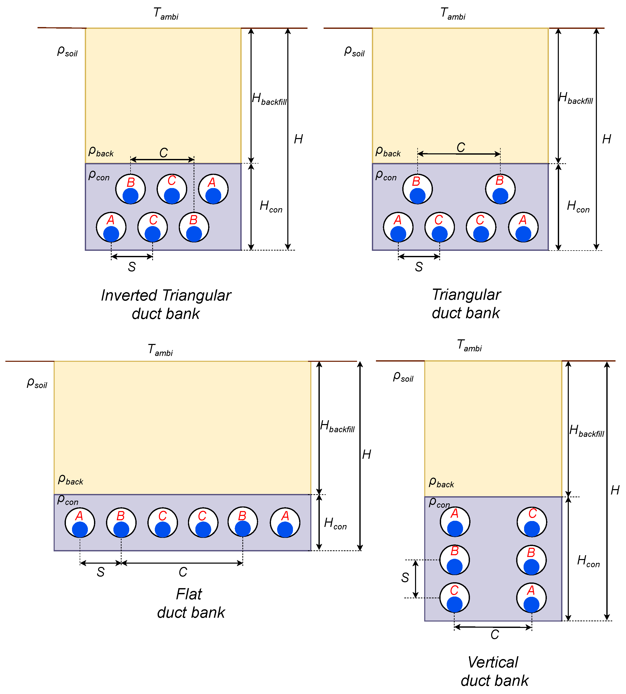
For this study, we used the four most frequently employed duct banks for double-circuit transmission lines with phase transposition, which are illustrated in Figure 1.
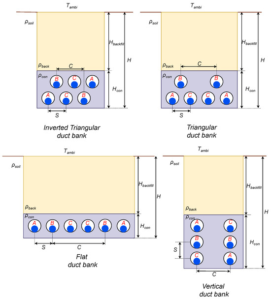
Figure 1.
Duct banks for double-circuit underground transmission lines.
In Figure 1, we have the phase separation denoted as S; the backfill depth identified as , commonly referred to as the free depth; and the depth of the concrete duct marked as . Additionally, the duct bank incorporates three distinct thermal resistivity values: , , and , corresponding to the backfill, concrete, and natural soil, respectively. represents the ambient temperature at the location, while the parameter C represents the separation between circuits.
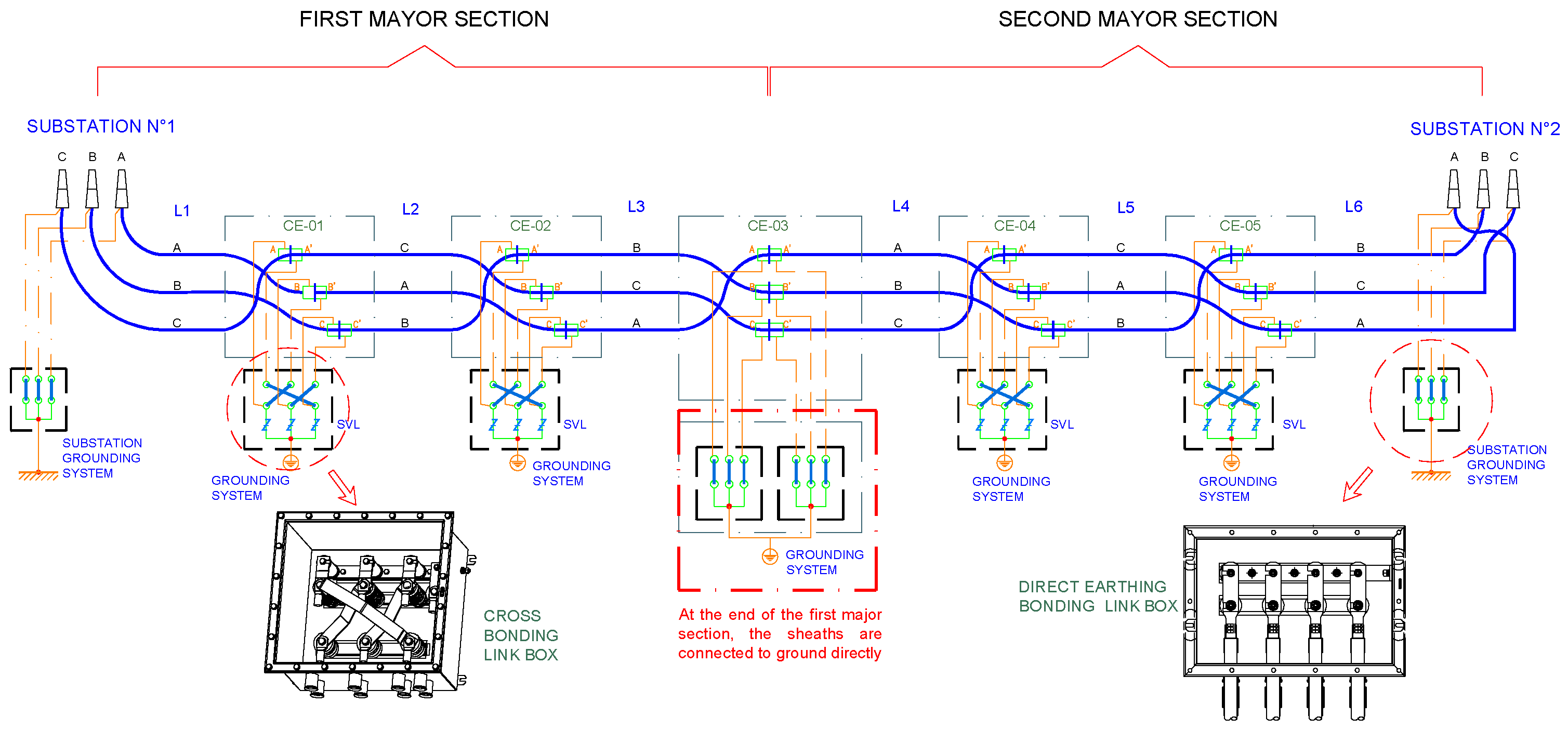
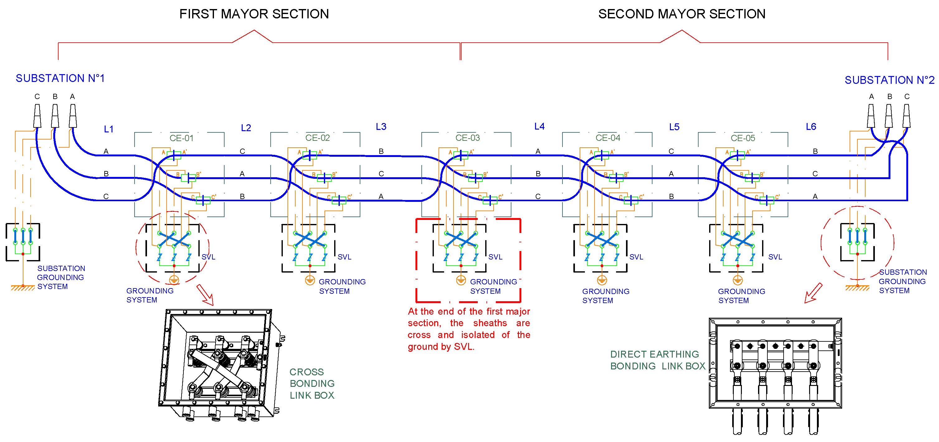
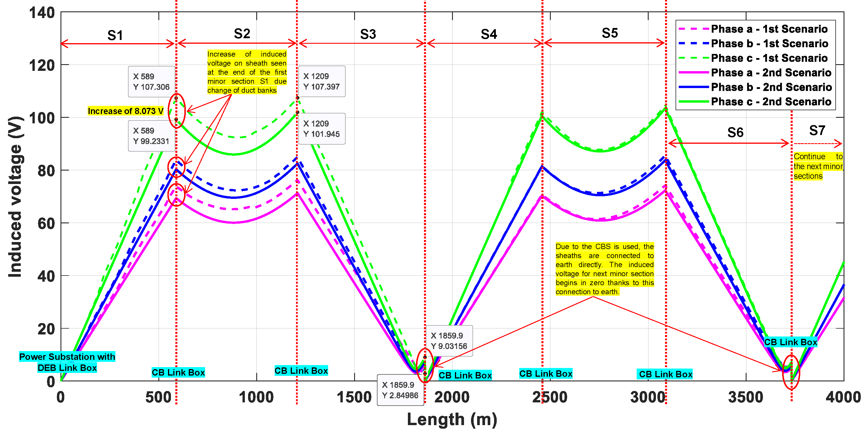
Additionally, to ensure the proper operation of the cable, specifically in terms of enhancing sheath voltage distribution and reducing sheath currents, the typical system used for grounding the sheaths is cross-bonding, as detailed in [6,17]. In the cross-bonding arrangement, electrically continuous sheaths run from earthed termination to earthed termination, but the sheaths are sectionalized and cross-connected to reduce sheath circulating currents and losses. Typically, the cable is divided into sections of approximately the same length. The sheaths at both ends of each section are grounded or isolated from the ground in their appropriate link boxes according to the type of cross-bonding. This cross-bonding of cable sheaths between sections almost eliminates induced voltage. These sections, called minor sections, collectively in groups of three form major sections. Multiple major sections may be used along a route depending on the total length of the cable. It is not generally possible to divide the route length into exactly matched minor section lengths, nor is it always possible to maintain a constant spacing of the cables throughout the route. Two typical cross-bonding methods are shown in Figure 2 and Figure 3. The sheaths are grounded but not cross-connected between major sections in the sectionalized cross-bonding (SCB) method (Figure 2). On the other hand, in the continuous cross-bonding (CCB) method (Figure 3), the sheaths are cross-connected but not directly grounded between major sections. This important difference between the two types of CB is highlighted in red in these figures.
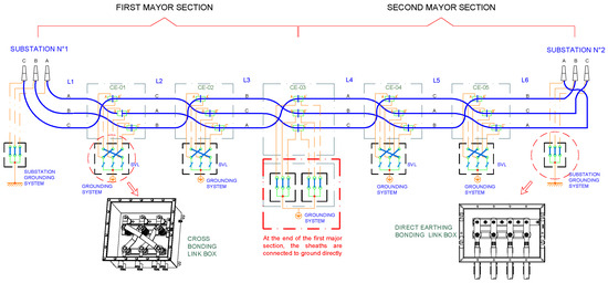
Figure 2.
Sectionalized cross-bonding method with typical cable transposition.
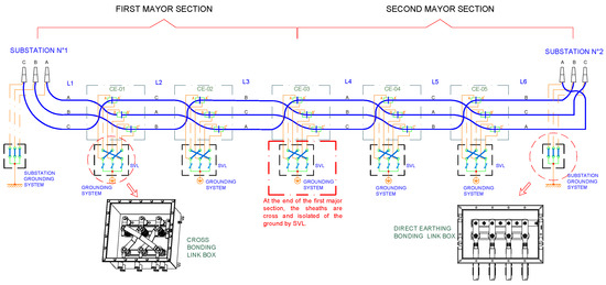
Figure 3.
Continuous cross-bonding method with typical cable transposition.
3. Situations Requiring Changes to Duct Bank Configuration and Cable Spacing
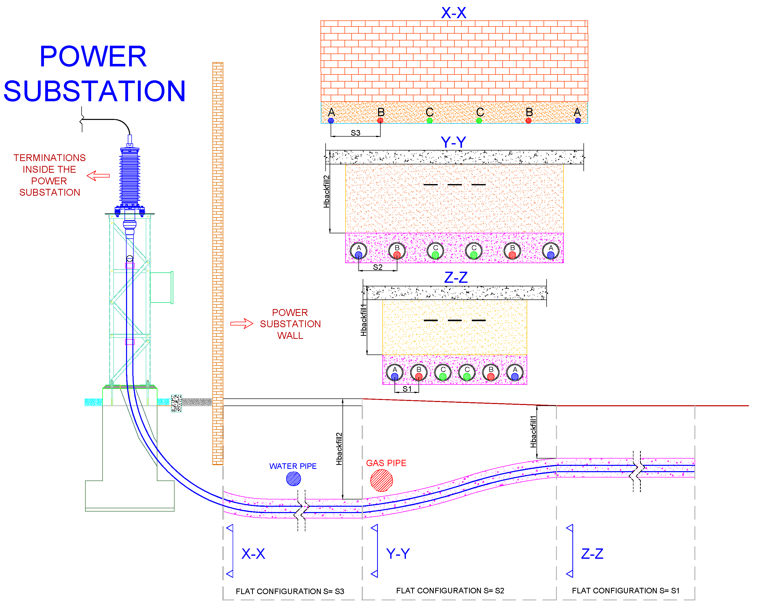
Due to underground obstructions, the dimensions of duct banks must increase the distance between cables to guarantee the current rating. Furthermore, for the entrance to a power substation, the distance between cables increases due to the separation of the termination inside the substation, as shown in Figure 4.
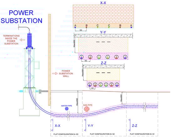
Figure 4.
Entrance to the power substation.
Figure 4 begins with a flat duct bank with a separation and depth ; due to the presence of a gas pipe, the duct bank goes deeper and increases the distance between cables (), as shown in Section Y-Y. After that, due to the presence of a large wall outside the substation and the distance between termination inside the substation, the cables have to be separated, as shown in Section X-X. In these cases, the distance between cables increases but the type of duct bank does not change.
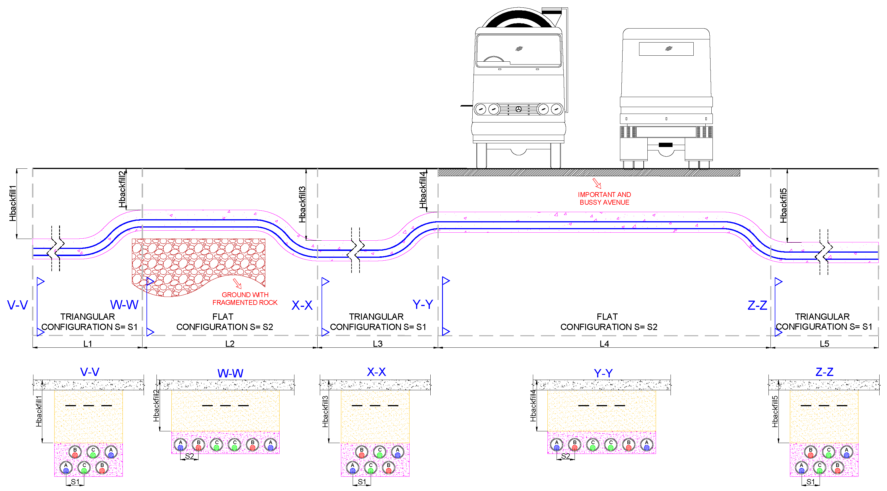
However, there are some important cases where the type of duct bank must be changed, considering two aspects: the economics and construction time. For example, when the ground has fragmented rock, it is difficult to excavate, which increases the costs and time of civil works. In this regard, it is necessary to change to a different duct bank that entails less excavation, as shown in Section W-W of Figure 5, over a length denoted as . After crossing this type of ground, the duct bank returns to its original configuration, as shown in Section X-X. Another scenario is when the underground transmission line has to cross an important avenue where it is necessary to perform all the civil work as soon as possible; in this scenario, the duct bank usually changes, as shown in Section Y-Y for a length . After crossing this important avenue, the duct bank returns to its original configuration, as shown in Section Z-Z.
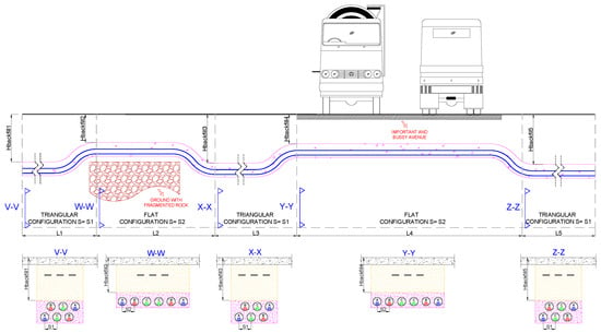
Figure 5.
Scenarios where the type of duct bank changes.
In summary, different working conditions generate changes in the pipeline layout (increase in the separation between cables or changes of duct bank), and whatever changes are carried out, the induced voltage will be affected.
The dimensions of the duct bank indicated in Sections V-V, W-W, X-X, Y-Y, and Z-Z are shown in Figure 4 and Figure 5; for example, the separation between cables Si and Hbackfilli depends of the condition and requirements of the project such as current rating, type of cable, thermal resistivity, and others. Once an ampacity analysis calculates the dimensions of the duct bank, it is possible to calculate the induced voltage along the underground transmission line.
4. Results
This section is divided into two parts. In the Ampacity Calculation subsection, we design and calculate the dimension of the duct banks usually used in a double-circuit underground transmission line (Figure 1). In the Induced Voltage Calculation subsection, we use the dimensions of the duct banks found in the previous subsection to calculate the induced voltage on the sheath.
4.1. Ampacity Calculation
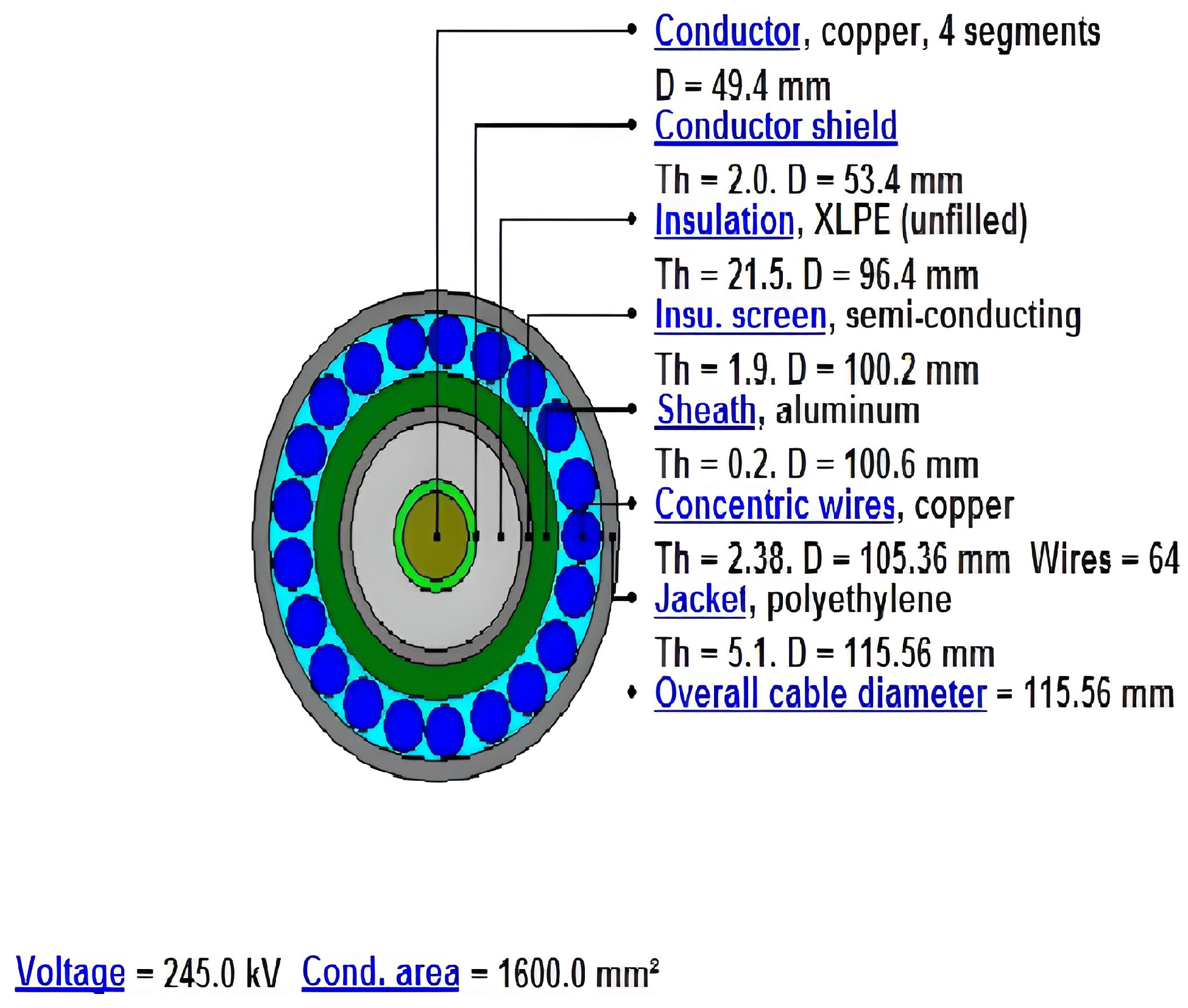
For this calculation, we used a real cable that utilizes a 220 kV single core for a double circuit with a 1600 mm2 copper core, XLPE insulation, and a 240 mm2 copper sheath. The ampacity required is 1000 A per circuit, and the thermal resistivity of the natural soil considered for the design is 2.7 K·m/W, while for the backfill, we employed 0.9 K·m/W. The value of the thermal resistivity of the concrete duct that surrounds the HDPE corrugated pipe is 0.75 K·m/W. The diameter of the HDPE pipe is 0.254 m (10 inches).
To resemble the installation conditions of an underground transmission line in a city, Table 1 presents underground obstructions that cross the underground transmission line transversely and longitudinally. Furthermore, due to the underground nature of the transmission line, most of the time, it has to cross important and busy avenues in a city; it will cross one lane at a time, always leaving a lane free to passing vehicles. However, vehicle traffic is still impacted, even when one lane is left open. In this regard, towns frequently ask for and occasionally require the concessionary firms in charge of underground transmission lines to complete the necessary work at the aforementioned crossings as soon as is feasible. Because of this, even if one duct bank is more expensive than another, some companies will employ it because it requires the least time for civil work. The flat duct bank is usually the one under consideration. Due to the low value of H, this duct bank usually does not require the realization of shoring (depending on ground type). In other words, after excavating and profiling the trench, the HDPE pipes can start being placed. Due to the absence of this activity, the time needed for civil works decreases, even though it is necessary to excavate more (a machine excavator usually performs this activity and is faster than shoring, which workers perform). Furthermore, in some cases, the underground transmission line has to pass through ground that is difficult to excavate, such as ground with fragmented rock. In such ground conditions, opting for a duct bank that demands shallower excavation depths is recommended. This choice is because, aside from requiring machine excavation, it would also necessitate the use of a hydraulic breaker to achieve the required depth specified by H. Employing both of these machines during excavation would extend the project timeline and elevate investment costs, primarily due to the high expenses associated with excavation. In simpler terms, the flat duct bank is the preferred option in these situations.

Table 1.
Depths of installation for underground obstructions.
Table 1 presents underground obstructions, intersections with important and busy avenues, and zones with a high cost of excavation. In all these interference zones, flat duct banks will be used.
As mentioned in the previous section, as long as the depth of installation increases, the ampacity will decrease. To avoid this decrease, it is necessary to increase the separation distance between cables. To calculate this increase in distance, the program Cymcap is required. Cyme International developed this software, which incorporates the IEC 60287 methodology for ampacity calculations and the finite element method for modeling and estimates the effect of backfill on the thermal resistance , which corresponds to the thermal resistance of the external medium of the duct (concrete and backfill when the duct banks are used). The program Cymcap has two ways to show results in its interface, depending on the input data and the result required. The first is when the result is the maximum current that the cable can transport without surpassing the maximum temperature, and the second one is the maximum temperature that the cable achieves when transporting the rated current. In our analysis, we used the second one because the goal was to transport the current rating. Most of the time, the first way is used when necessary to verify the ampacity of cables in duct banks already constructed.
Figure 6 shows the cable modeling within Cymcap with all its parts, such as core, semiconductive layers, sheath, and jacket, while Figure 7 shows an example of the second way Cymcap shows the results of the calculation of the ampacity considering the data inputs, the depth, and the separation indicated.
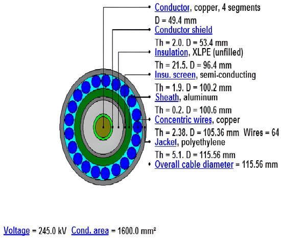
Figure 6.
Cable modeling of 220 kV using Cymcap considering the dimensions of the cable.

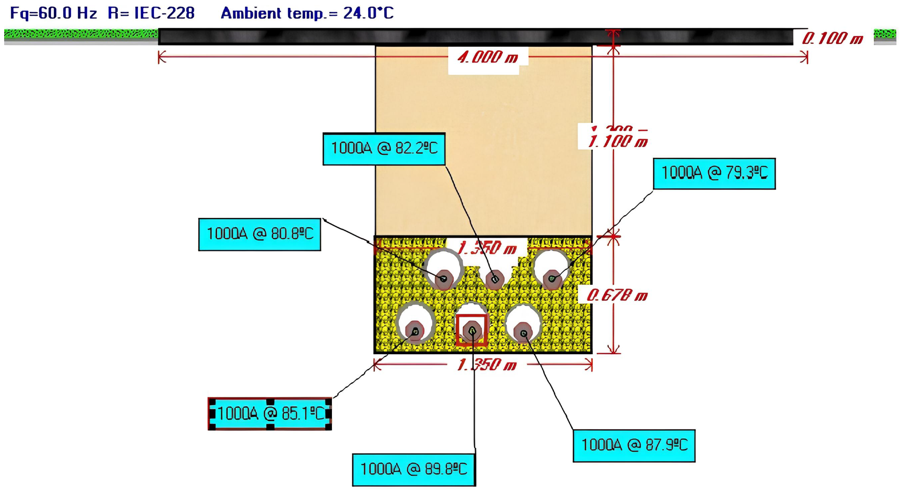
Figure 7.
Calculation of ampacity of the inverted triangular duct bank with S = 350 mm.
Figure 7 illustrates the ampacity result for an inverted triangular duct bank. In this configuration, the cable in phase C in the first circuit consistently attains the maximum temperature recommended by the manufacturer for XLPE insulation, which is typically set at 90 °C. It is sufficient for any cable within a circuit to reach its maximum temperature to determine the maximum current the underground transmission line can carry. The cable in phase C, considering the distribution phases in Figure 1 in the first circuit (the left one), reaches this maximum temperature first because, around itself, there are four heat sources (cables that also transport current). On the other side, the cable in phase A in the second circuit is the one that transports the current rating with the low temperature because it just has two heat sources around itself and is installed at the top of the duct. The most important value in this analysis is the maximum free depth, also known as the backfill depth , that the duct bank has that allows the transport of the current rating. In this case, 1.20 m is measured from the ground’s superficial level to the top of the duct bank. Therefore, the maximum free depth for the inverted triangular duct bank with a separation between cables of 350 mm is 1.20 m. This procedure was applied for the four duct bank types frequently used in double circuits in underground transmission lines, considering an increase of 0.10 m of the maximum depth of installation of obstructions shown in Table 1. This extra value corresponds to the gap between the interference and the top of the duct bank, which is a good practice during the construction of duct banks. As it is a good practice, this value will increase or decrease according to each project’s design and construction criteria. The result of this ampacity evaluation is in Table 2.
Table 2.
Dimensions for each type of duct bank.
The results show that the maximum free depth depends on the cables’ separation and the duct bank type. For instance, the inverted triangular duct bank, which is the most compact duct bank, which has an S = 350 mm, allows the transport of the rated current at a maximum free depth of 1.2 m. After reaching this depth, increasing the separation following the depth requirements becomes necessary. Moreover, due to the inverted triangular type being compact, when considering a separation S = 300 mm with = 1000 mm, it cannot transport the current rating. Furthermore, because the cables in the center of the duct only have two heat sources surrounding them, the flat duct bank only needs a spacing of S = 300 mm to convey the current rating up to 1.80 m as free depth.
4.2. Induced Voltage on Sheath Calculation
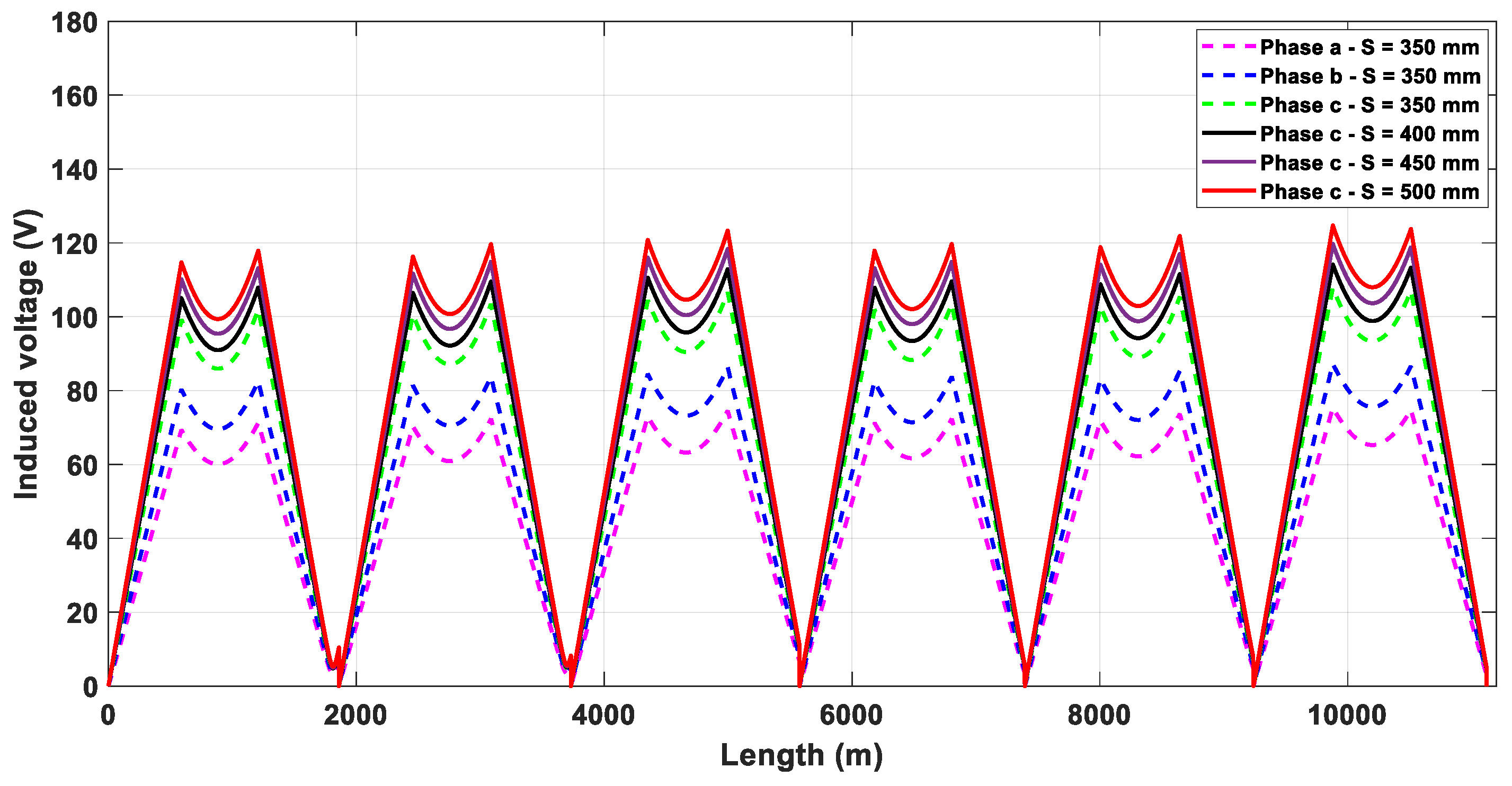
In order to compute the induced voltage, applying the mathematical formulas presented in [16,18] for a double circuit with phase transposition, it is possible to calculate the induced voltages on the cable sheath as long as the separation between cables increases. In that sense, using the software MATLAB R2021b version and considering the minor section lengths presented in Table 3, Figure 8 presents the profile of induced voltage on the sheath of an underground transmission line, assuming that there are no underground obstructions in the route and using only the inverted triangular duct bank with four different separation distances between cables of S = 350, 400, 450, and 500 mm.
Table 3.
Minor section lengths for each major section of underground transmission line.
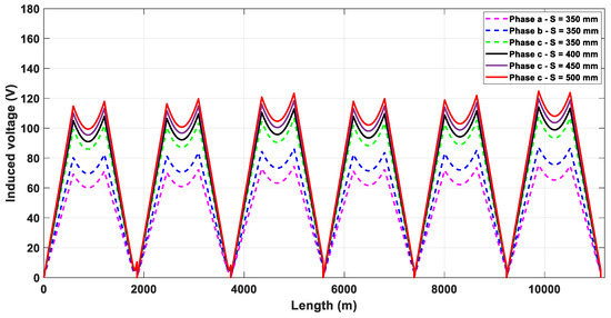
Figure 8.
Induced voltage profile of inverted triangular duct bank with different separation distances.
As shown in Figure 8, for S = 350 mm, the figure presents the profile of the three phases, where phase C presents the high value of induced voltage. For the other separations (400, 450, and 500 mm), just the maximum value of the induced voltage (in phase C) is presented to show the impact of increasing the separation between phases. In conclusion, the induced voltage on a sheath increases as long as the distance between phases increases. This increase depends on the type of duct bank, the cable dimensions, and the current rating.
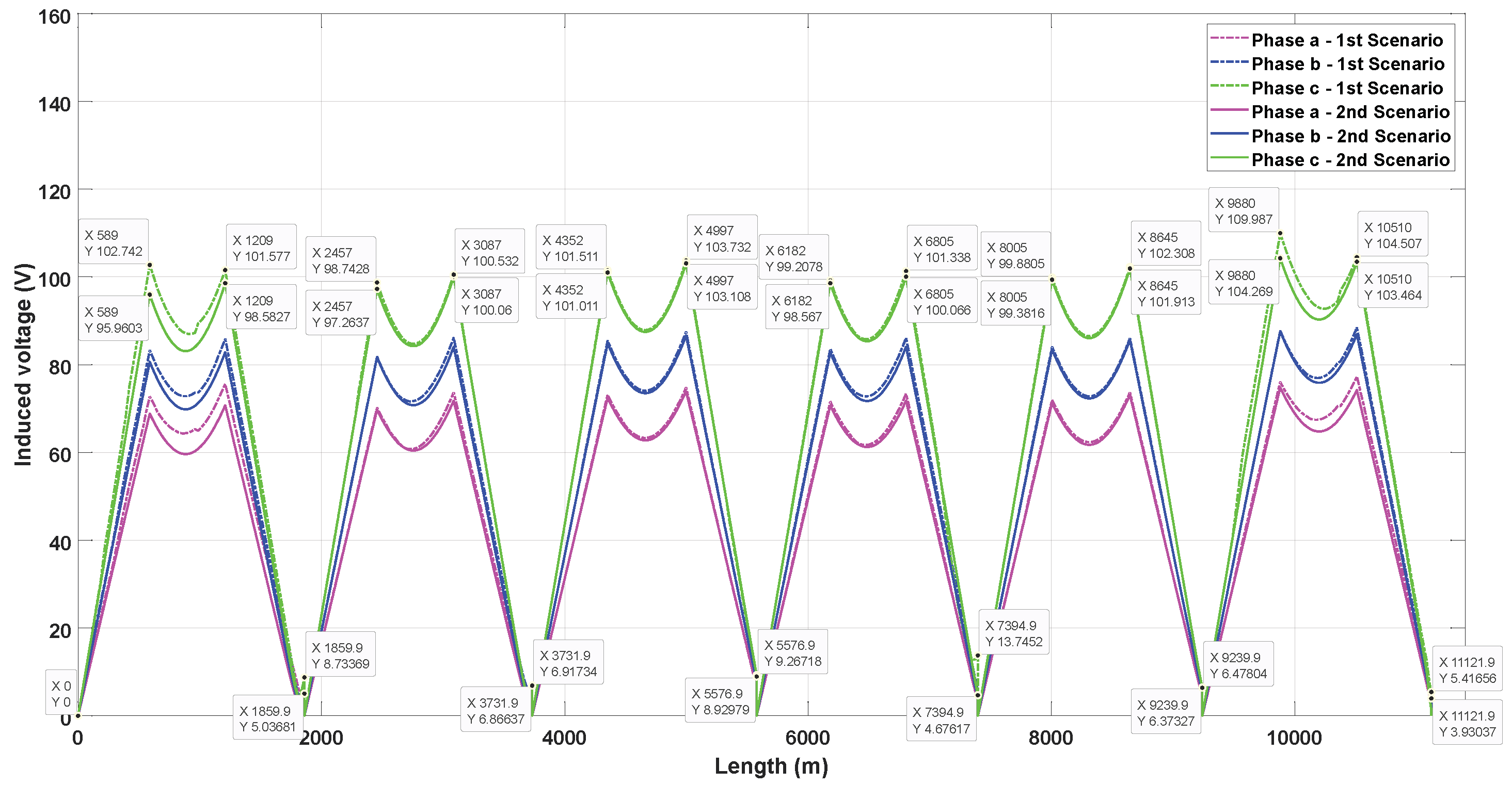
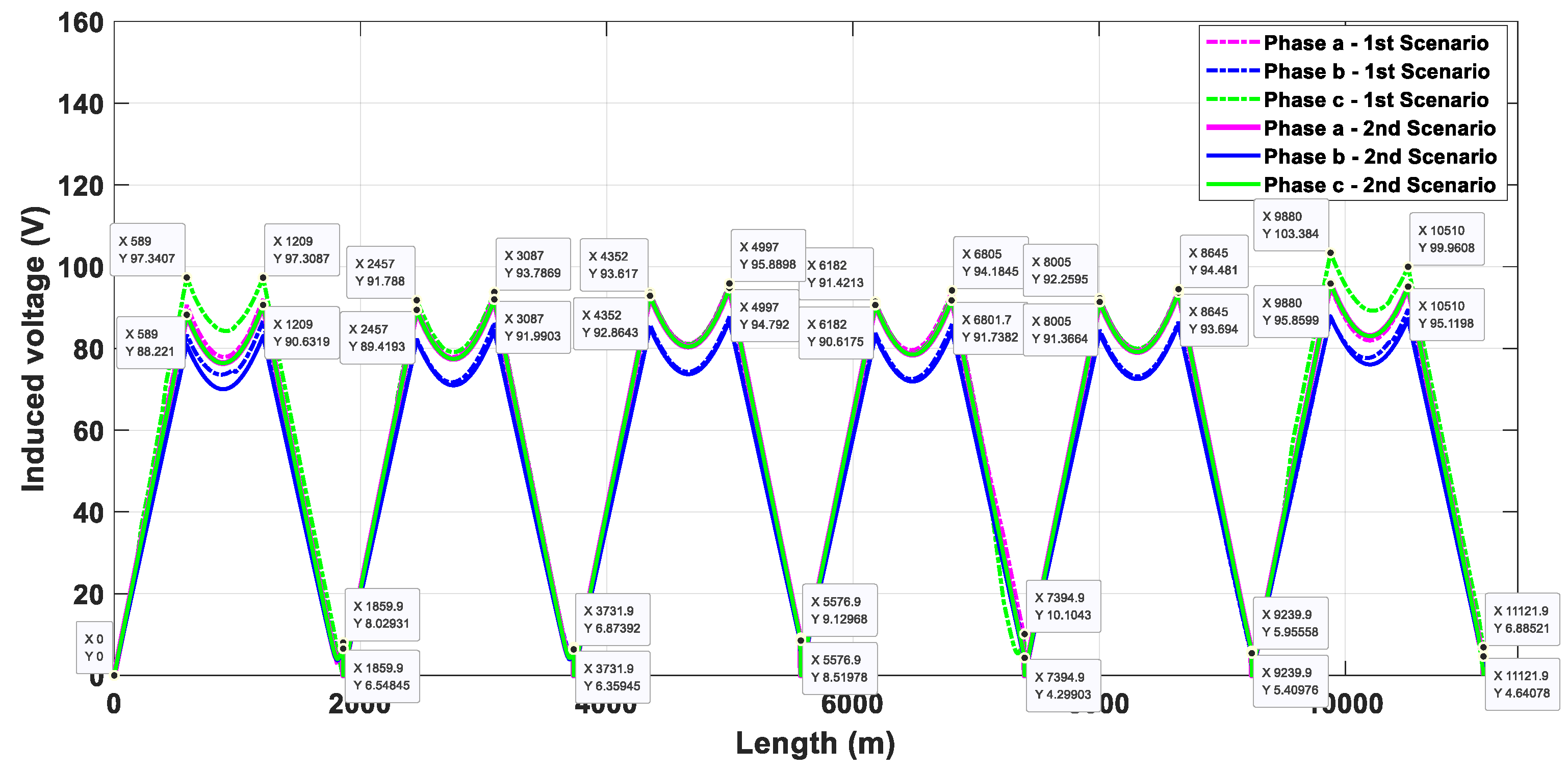
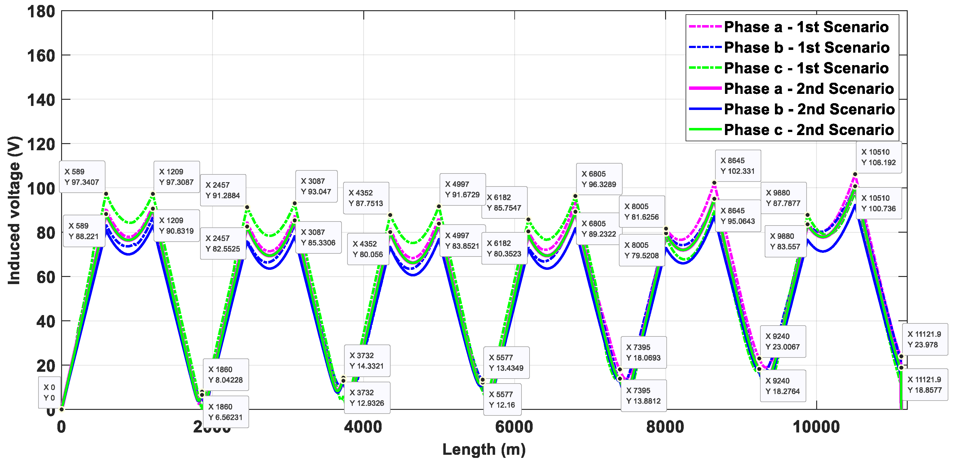
In order to calculate the impact of the change of duct bank type along the route of an underground transmission line on the induced voltage on the sheath, we made up two distinct scenarios. In scenario 1, the most accurate calculation methodology, we considered the impact of the induced voltage on the sheath due to the increase in the separation between cables and change of the duct bank to a flat one, according to what is indicated in Table 1. This table shows situations that involve the of changing the duct bank, which could be due to an underground obstruction, an intersection with a busy avenue, or high excavation costs. In scenario 2, we only considered one duct bank with a unique separation distance, even though this is not real; in other words, obstructions to and a change of the duct bank were not considered. This is the methodology normally used to calculate the induced voltage on a sheath. For instance, a separation of 350 mm between cables was employed for the inverted triangular duct bank. In contrast, a separation of 300 mm was utilized for the other duct banks. However, for the flat duct bank, due to the minimum separation, S = 300 mm allows the transport of the current rating up to 1.80 m as free depth. Both scenarios are the same. For both scenarios, for the four duct banks, both types of cross-bonding were used, sectionalized (SCB) and continuous (CCB). The results of the induced voltage on the sheath are illustrated in Figure 9, Figure 10, Figure 11, Figure 12, Figure 13, Figure 14, Figure 15 and Figure 16. Meanwhile, Figure 17 shows the curves of induced voltages on the sheath in just the first seven minor sections (Si) for both scenarios in order to clearly explain the results.
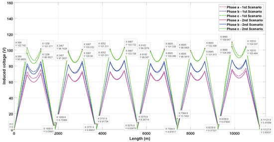
Figure 9.
Induced voltages on sheath in triangular duct bank with phase transposition with sectionalized cross-bonding.
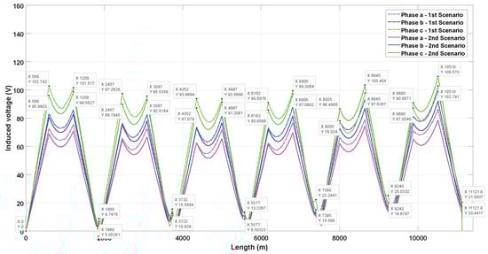
Figure 10.
Induced voltages on sheath in triangular duct bank with phase transposition with continuous cross-bonding.
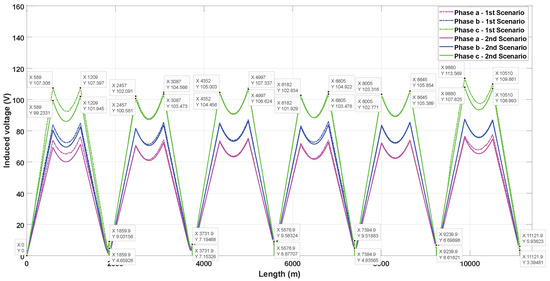
Figure 11.
Induced voltages on sheath in inverted triangular duct bank with phase transposition with sectionalized cross-bonding.

Figure 12.
Induced voltages on sheath in inverted triangular duct bank with phase transposition with continuous cross-bonding.
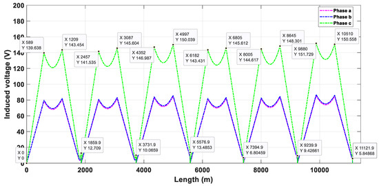
Figure 13.
Induced voltages on sheath in flat duct bank with phase transposition with sectionalized cross-bonding.
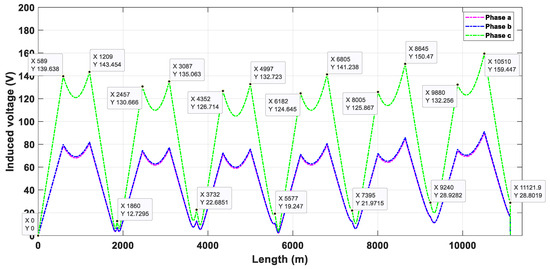
Figure 14.
Induced voltages on sheath in flat duct bank with phase transposition with continuous cross-bonding.
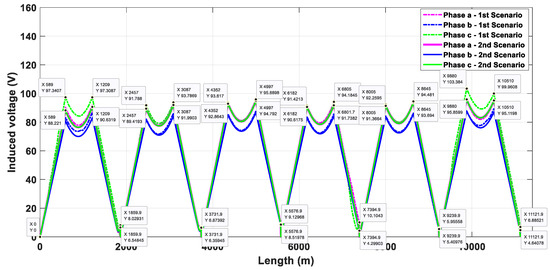
Figure 15.
Induced voltages on sheath in vertical duct bank with phase transposition with sectionalized cross-bonding.
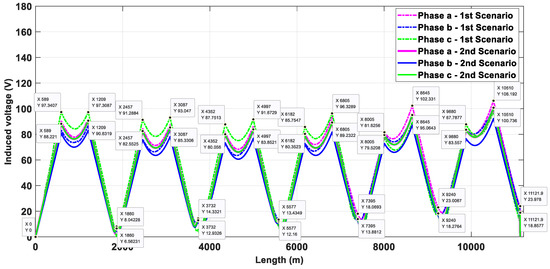
Figure 16.
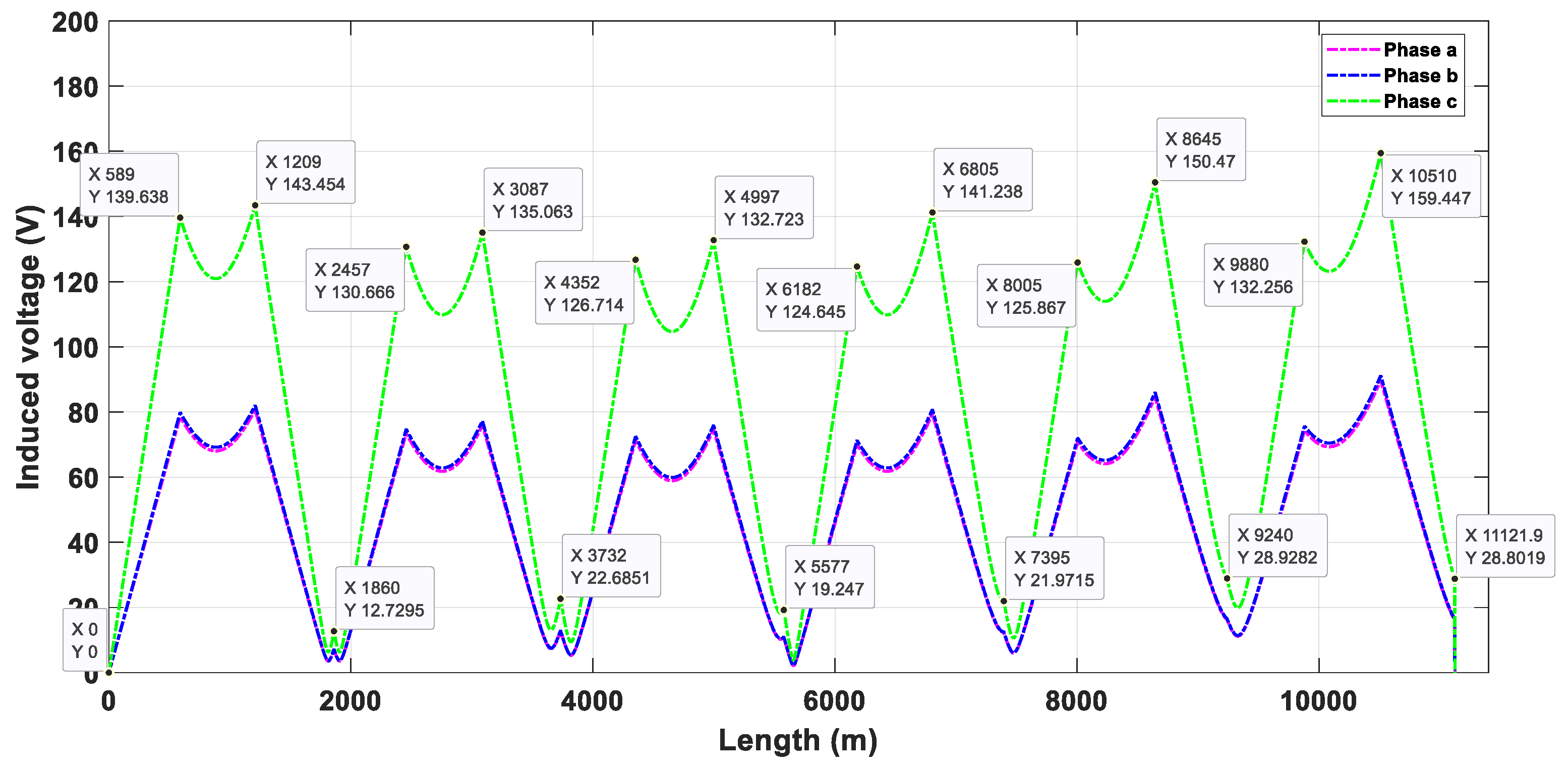
Induced voltages on sheath in vertical duct bank with phase transposition with continuous cross-bonding.
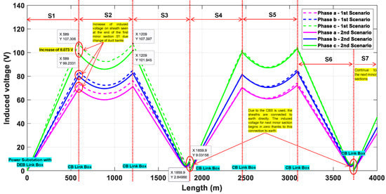
Figure 17.
Induced voltage on sheath curves.
Figure 17 shows a triangular duct bank with sectionalized cross-bonding. The induced voltage on the sheath curves of the three phases begins in the power substation with 0 V; as long as the length increases, this value will constantly increase if we focus on the second case; nevertheless, if we focus on scenario 1, this increase will be variable, depending of the change of duct bank and the increase in distance between cables. The end of the first minor section () in Figure 17 presents an increase of 8.073 V in the sheath of phase C when scenario 1 is observed. The other two phases also increase in value. This value is measured in the first jointing box, where the cross-bonding technique is applied. The same occurs after the second minor section , where the increase is 5.45 V in phase C. At the end of the third minor section, , due to SCB being applied, the sheaths are connected directly to the earth, making the value of induced voltage zero. For the fourth minor section, , the induced voltage begins at zero because the sheaths are connected to the earth. If the bonding method had been CCB, the induced voltage in would begin at the residual voltage value and not at zero.
Additionally, Table 4 presents the summary of the results of the maximum value of the induced voltage on the sheath measured in the jointing box for the four common duct banks used considering both types of cross-bonding, SCB and CCB, and considering the phases identified in Figure 1. This table shows the maximum values of the two scenarios, the increase of induced voltage, and the representative phase, which is the one that has the maximum value of voltage between the three phases. It is easily notable that for all duct banks except for the flat one, there is an increase in induced voltage when the first is considered, where the greatest increase occurs in the vertical duct bank when SCB is applied. On the other side, the flat duct bank generates more induced voltage on the sheath; however, it is also the one that can be installed at a greater depth. Additionally, phase C is the one that generates a higher induced voltage on the sheath, except in the vertical duct bank; for this duct bank, phase A is representative.
Table 4.
Summary of induced voltage peak values on sheath across four common duct banks, considering both types of cross-bonding, SCB and CCB.
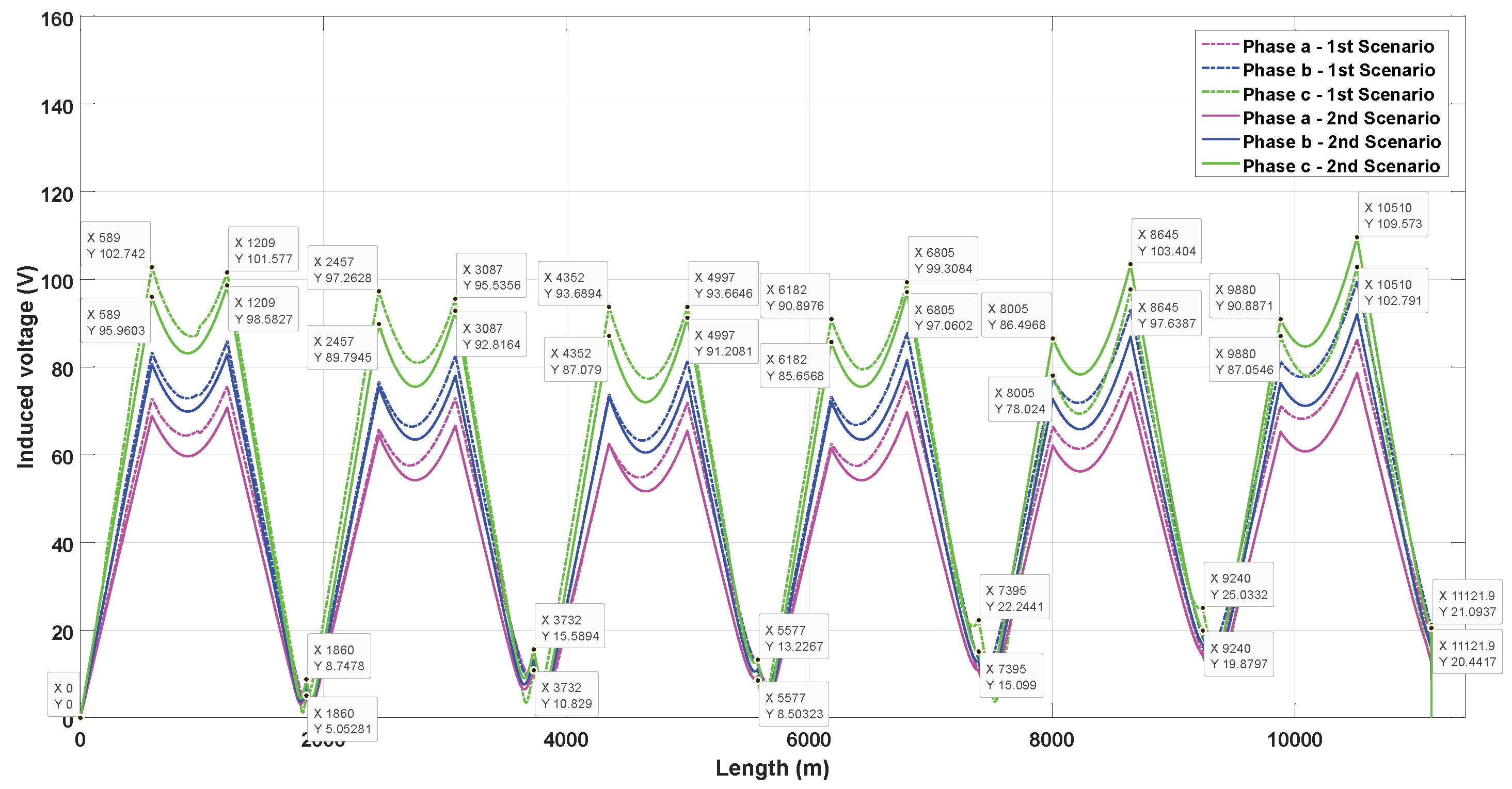
Figure 9 and Figure 10 show the induced voltages on the sheath within the triangular duct bank where the maximum value happens in phase C. In scenario 1, the highest value occurs at the end of the sixth major section’s first minor section (), reaching 109.98 V when SCB is used. Comparatively, with CCB, the highest value is 109.57 V and happens at the end of the second minor section () of the sixth major section. The residual induced voltage at the end of the last major section is 5.41 V when SCB is used and 20.44 V when CCB is used. This last value does not occur in phase C but in phase B. In scenario 2, using SCB, the peak value of induced voltage is 104.27 V, decreasing by 5.72 V (5.48%) compared to the first scenario, while using CCB, the peak value is 102.79 V, which means a decrease of 6.78 V (6.6%). Regarding the residual induced voltage, using SCB it is 3.93 V (1.48 V less than scenario 1), while when employing CCB, there is no important difference between both scenarios (0.65 V).
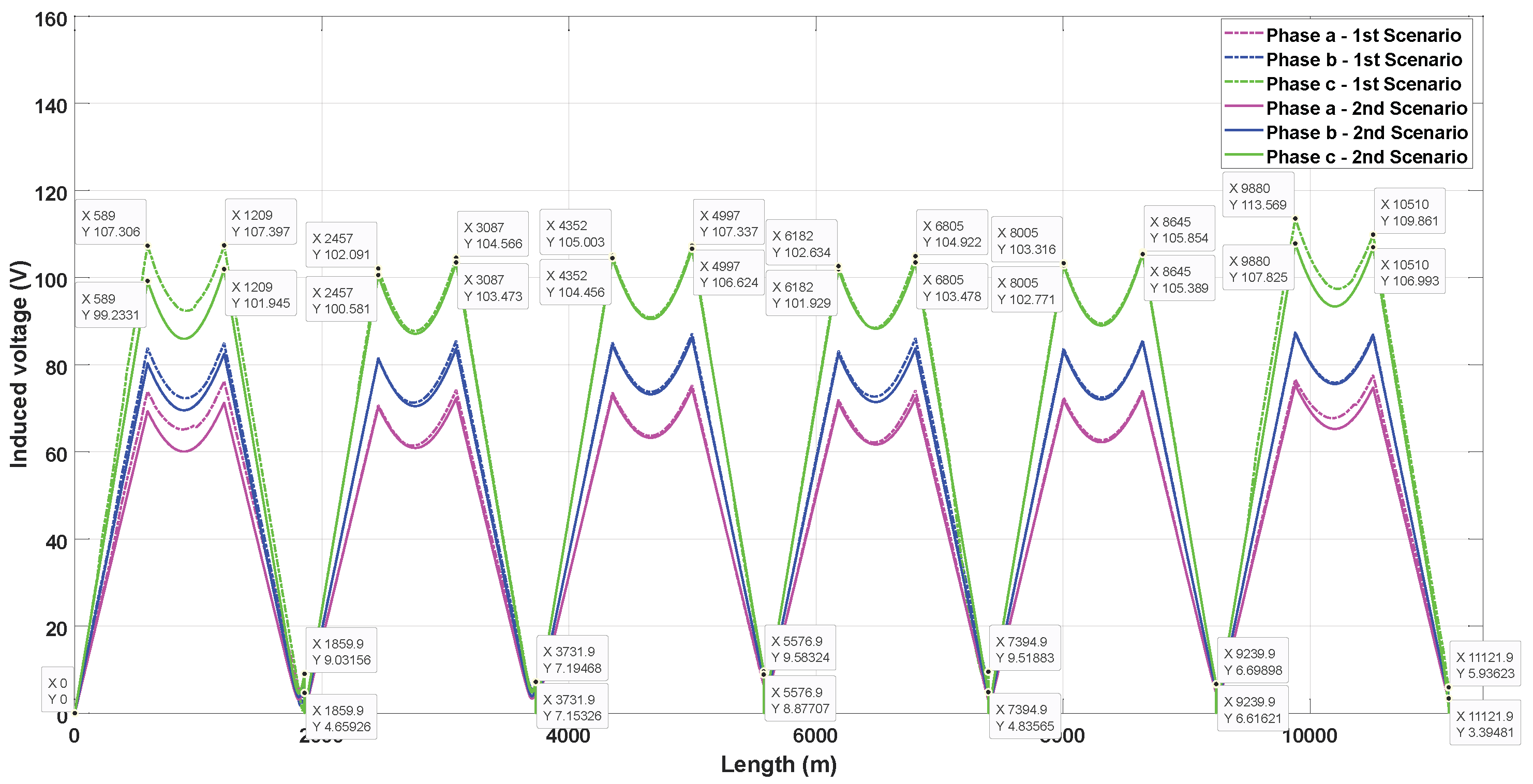
Figure 11 and Figure 12 show the induced voltages on the sheath within the inverted triangular duct bank, where the maximum value happens in phase C. In scenario 1, the highest value occurs at the end of the sixth major section’s first minor section (), reaching 113.57 V when SCB is used. Comparatively, with CCB, the highest value is 113.31 V and happens at the end of the sixth major section’s second minor section (). The residual induced voltage at the end of the last major section is 5.93 V when SCB is used and 20.31 V using CCB, and this last value does not occur in phase C; it occurs in phase B. In scenario 2, using SCB, the peak value of induced voltage is 107.82 V, decreasing by 5.74 V (5.33%) compared to scenario 1, while using CCB, the peak value is 110.98 V, which means a decrease of 2.33 V (2.10%). Regarding the residual voltage, when SCB is used, the residual voltage at the end of the last major section is 3.39 V (2.35 V less than scenario 1), while when employing CCB, there is no important difference between scenarios (0.03 V).
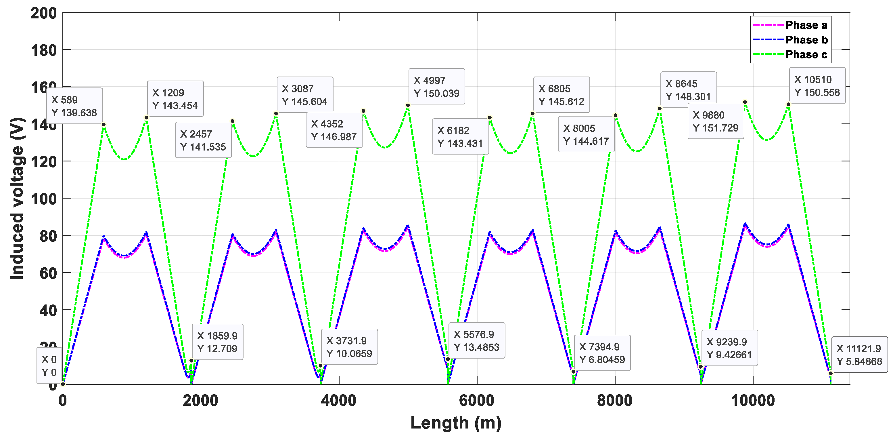
The flat duct bank is the one that transports more power with less separation distance between phases. However, this duct bank is the one that generates more induced voltages on the sheath, where the maximum value occurs in phase C, while the other two phases have almost identical values in their profile of induced voltages. As mentioned, due to the minimum value of the separation distance, this duct bank can cross all obstructions and busy avenues without varying this distance or the type of duct bank; hence, both scenarios are the same. Figure 13 and Figure 14 show the induced voltage on the sheath of this duct bank employing the two types of cross-bonding. When SCB is used, the maximum value of induced voltage is 151.73 V, while it is 159.44 V using CCB. Furthermore, there is a notable difference in the residual induced voltage on the sheath at the end of the underground transmission line (22.96 V), where using SCB obtained the lower value of residual induced voltage.
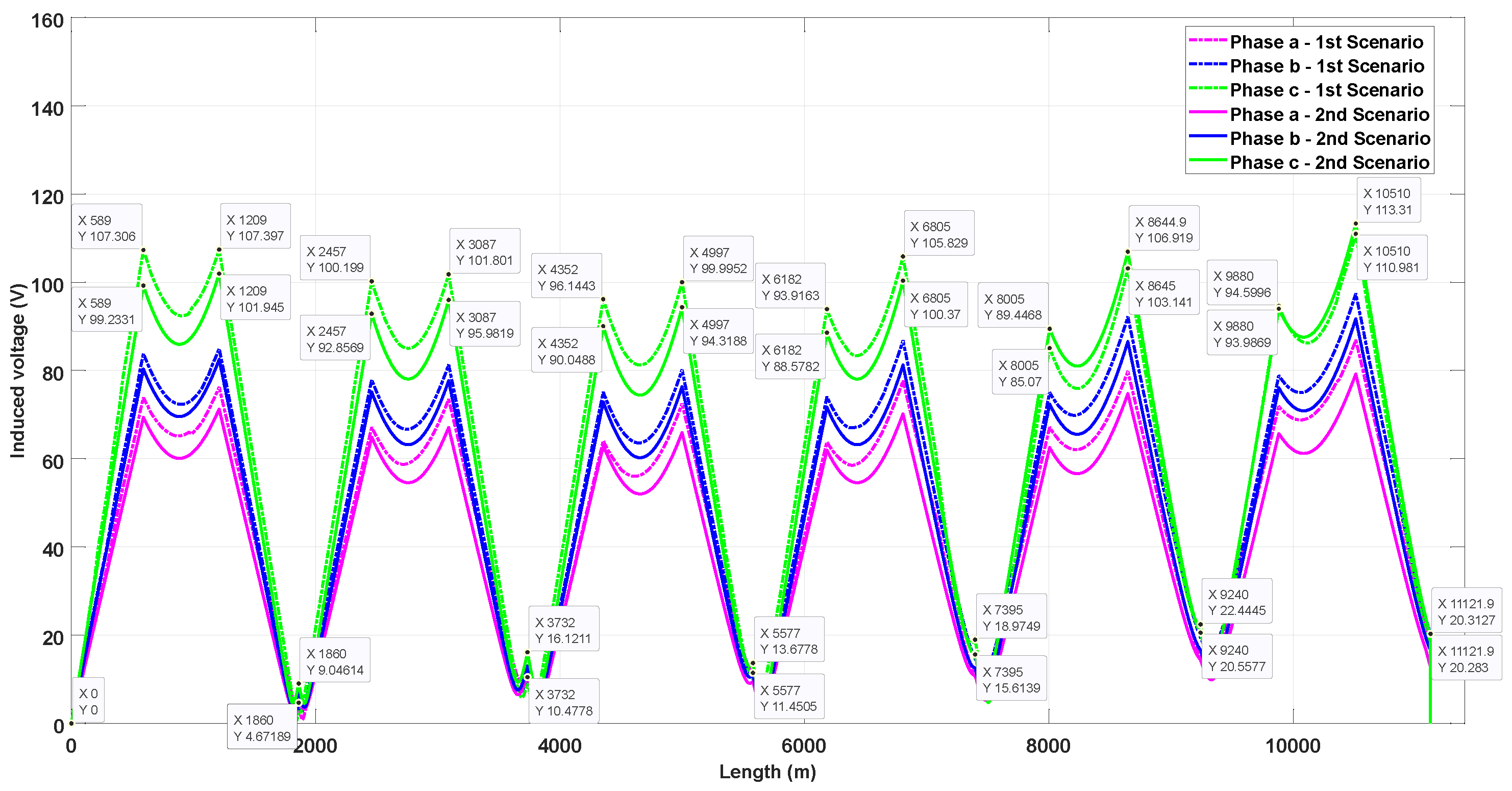
The induced voltages on the sheath when a vertical duct bank is used are presented in Figure 15 and Figure 16. In scenario 1, the high value of induced voltage also occurs at the end of the first minor section of the last major section () in phase C, reaching 103.38 V when SCB is used. On the other hand, using CCB, the maximum value occurs at the end of the second minor section of the last major section (), reaching 106.19 V in phase A. The residual induced voltage at the end of the last major section is 6.88 V when SCB is used and 23.98 V using CCB; this last value does not occur in phase C, it occurs in phase A. For scenario 2, the maximum value of induced voltages occurs in phases A and C, independent of the type of cross-bonding. Using SCB, the high value occurs at the end of the minor section value and decreases by 7.52 V (7.85%) in comparison with scenario 1, while the high value decreases by 5.45 V (5.41%) and occurs at the end of the minor section when CCB is used. Regarding the residual induced voltage, using SCB, the value decreases to 2.24 V, while when employing CCB it decreases to 5.12 V.
For all the duct banks, the highest value of induced voltage happens in the last major section because it requires changes to the flat duct bank, as can be observed in Table 1.
5. Conclusions
In this study, we carry out ampacity and induced sheath voltage calculations for an underground transmission line considering four double-circuit duct banks with both types of cross-bonding (sectionalized and continuous cross-bonding). The simulations performed for the ampacity calculation reveal that as long as the duct bank deepens, it is necessary to increase the separation distance between cables to ensure the current rating; however, the results of induced voltage calculation show that when this distance increases, the induced voltage on the sheath increases and is dependent on the duct bank configuration, the current rating, and the type of cross-bonding applied.
To demonstrate the impact of the increase of the induced voltage on the sheath due the change of duct bank, we analyzed two distinct scenarios. Scenario 1, which is the most exact and like a real case, considers all the increases due to underground obstructions and changes of duct bank. Scenario 2 assumes that there does not exist underground obstructions or changes in duct banks and only consider the typical duct bank. The results show that the high value of the induced voltage on the sheath in the first scenario is 7.85% higher than the second one when SCB is used. On the other hand, using CCB, the results obtained in scenario 1 are higher than scenario 2 by 6.6%. To obtain the residual induced voltage, using SCB, the results in scenario 1 are higher than the second one by 2.35 V, where the maximum value is 6.88 V when a vertical duct bank is used. Conversely, when CCB is used, the residual induced voltage increases to 23.97 V, which means more losses on the sheath than when using SCB. In that sense, and with the simulations, we show that CCB generates more losses on the sheath than SCB, which will increase if there are underground obstructions or changes of duct banks. Therefore, as a good design practice, calculating the induced voltage on the sheath using SCB is enough to carry out this calculation considering scenario 2 and then adding a factor such as 1.08, as a minimum, in the final result when the typical duct bank is in vertical configuration, 1.05 when triangular inverted is used, and 1.07 when a triangular configuration is applied.
Author Contributions
Conceptualization, J.E.G.A. and J.S.L.C.; methodology, J.E.G.A. and J.S.L.C.; software, J.E.G.A.; validation, J.E.G.A. and J.S.L.C.; formal analysis, J.E.G.A. and J.S.L.C.; investigation, J.E.G.A. and J.S.L.C.; writing—original draft preparation, J.E.G.A. and J.S.L.C.; visualization, J.E.G.A., J.S.L.C. and S.K.; supervision, J.S.L.C., J.P.F. and S.K.; project administration, J.E.G.A., J.S.L.C., J.P.F. and S.K.; funding, J.E.G.A., J.S.L.C. and S.K. All authors have read and agreed to the published version of the manuscript.
Funding
This work was funded by the Coordenação de Aperfeiçoamento de Pessoal de Nível Superior—Finance code 001 and the São Paulo Research Foundation (FAPESP) grants: 2021/06157-5 and 2023/05066-1.
Data Availability Statement
Data are contained within the article.
Conflicts of Interest
The authors declare no conflicts of interest.
Abbreviations
The following abbreviations are used in this manuscript:
| CCB | continuous cross-bonding |
| SCB | sectionalized cross-bonding |
| GIS | gas-insulated substation |
| SVL | sheath voltage limiter |
| FEM | finite element method |
| DEB | direct earthing bonding |
| CB | cross-bonding |
References
- Moutassem, W.; Anders, G.J. Configuration Optimization of Underground Cables for Best Ampacity. IEEE Trans. Power Deliv. 2010, 25, 2037–2045. [Google Scholar] [CrossRef]
- Anders, G.J.; Electrical, I.; Engineers, E. Rating of Electric Power Cables in Unfavorable Thermal Environment; Wiley: Hoboken, NJ, USA, 2005. [Google Scholar]
- Perović, B.; Klimenta, D.; Tasić, D.; Raičević, N.; Milovanović, M.; Tomović, M.; Vukašinović, J. Increasing the ampacity of underground cable lines by optimising the thermal environment and design parameters for cable crossings. IET Gener. Transm. Distrib. 2022, 16, 2309–2318. [Google Scholar] [CrossRef]
- Noufal, S.M.; Anders, G.J. Sheath losses correction factor for cross-bonded cable systems with unknown minor section lengths: Analytical expressions. IET Gener. Transm. Distrib. 2021, 15, 849–859. [Google Scholar] [CrossRef]
- IEEE Std 575; IEEE Guide for Bonding Shields and Sheaths of Single-Conductor Power Cables Rated 5 kV through 500 kV. IEEE: Piscataway, NJ, USA, 2014.
- CIGRE WG B1.50; Sheath Boding Systems of AC Tranmsision Cables–Design, Testing, and Maintanence. Technical Brochure 797; CIGRE: Paris, France, 2020.
- Candela, R.; Gattuso, A.; Mitolo, M.; Sanseverino, E.R.; Zizzo, G. A Model for Assessing the Magnitude and Distribution of Sheath Currents in Medium and High-Voltage Cable Lines. IEEE Trans. Ind. Appl. 2020, 56, 6250–6257. [Google Scholar] [CrossRef]
- Brakelmann, H.; Anders, G.J. Ampacity Calculations of Underground Power Cables With End Effects. IEEE Trans. Power Deliv. 2023, 38, 1968–1976. [Google Scholar] [CrossRef]
- Hoerauf, R. Ampacity application considerations for underground cables. In Proceedings of the 2015 IEEE/IAS 51st Industrial & Commercial Power Systems Technical Conference (I&CPS), Calgary, AB, Canada, 5–8 May 2015; pp. 1–9. [Google Scholar] [CrossRef]
- Alexandrou, K.; Anders, G. Sheath circulating currents calculation in asymmetrical installation schemes for power frequency models. In Proceedings of the10th International Conference on Insulated Power Cables, Versailles, France, 23–27 June 2019. [Google Scholar]
- Ocłoń, P.; Cisek, P.; Pilarczyk, M.; Taler, D. Numerical simulation of heat dissipation processes in underground power cable system situated in thermal backfill and buried in a multilayered soil. Energy Convers. Manag. 2015, 95, 352–370. [Google Scholar] [CrossRef]
- IEC 60287-2-1; Electric Cables—Calculation of the Current Rating—Part 1-1: Current Rating Equations (100% Load Factor) and Calculation of Losses—General. IEC: Geneva, Switzerland, 1995.
- IEEE 835; IEEE Standard Power Cable Ampacity Tables. IEEE: Piscataway, NJ, USA, 1994.
- de Leon, F.; Anders, G.J. Effects of Backfilling on Cable Ampacity Analyzed With the Finite Element Method. IEEE Trans. Power Deliv. 2008, 23, 537–543. [Google Scholar] [CrossRef]
- Cymcap Version 8.1 for Windows, CYME Int. T&D, Dec. 2017 St. Bruno, QC, Canada. 2017. Available online: https://www.cyme.com/ (accessed on 17 March 2023).
- Guevara, J.E.; Colqui, J.S.L.; Bautista, J.P.; Filho, J. Analysis of Induced Voltages and Currents on the Sheath of Double-Circuit Underground Power Lines—Part II: With Phases Transposition. In Proceedings of the 2023 IEEE XXX International Conference on Electronics, Electrical Engineering and Computing (INTERCON), Lima, Peru, 2–4 November 2023. [Google Scholar]
- Candela, R.; Gattuso, A.; Mitolo, M.; Sanseverino, E.R.; Zizzo, G. A Comparison of Special Bonding Techniques for Transmission and Distribution Cables. In Proceedings of the 2020 IEEE International Conference on Environment and Electrical Engineering and 2020 IEEE Industrial and Commercial Power Systems Europe (EEEIC/I&CPS Europe), Madrid, Spain, 9–12 June 2020; pp. 1–6. [Google Scholar] [CrossRef]
- Guevara, J.E.; Colqui, J.S.L.; Bautista, J.P.; Filho, J.P. Analysis of Induced Voltages and Currents on the Sheath of Double-Circuit Underground Power Lines-Part I: Without Phases Transposition. In Proceedings of the 2023 IEEE XXX International Conference on Electronics, Electrical Engineering and Computing (INTERCON), Lima, Peru, 2–4 November 2023. [Google Scholar]
Disclaimer/Publisher’s Note: The statements, opinions and data contained in all publications are solely those of the individual author(s) and contributor(s) and not of MDPI and/or the editor(s). MDPI and/or the editor(s) disclaim responsibility for any injury to people or property resulting from any ideas, methods, instructions or products referred to in the content. |
© 2024 by the authors. Licensee MDPI, Basel, Switzerland. This article is an open access article distributed under the terms and conditions of the Creative Commons Attribution (CC BY) license (https://creativecommons.org/licenses/by/4.0/).