
Detection of Non-Technical Losses on a Smart Distribution Grid Based on Artificial Intelligence Models
 , ,
, ,  , , , , and
Abstract
:1. Introduction
- Fraud: When a consumer attempts to deceive an electric power utility. This is usually carried out by tampering with energy meters, making them register a lower electricity energy consumption than actually consumed;
- Bypass: The bypass is a clandestine connection made directly from the power grid to the load, without passing through the energy meter;
- Bribery: Bribing power utility employees is another common practice. Corruption can come from both the consumer and the employee;
- Non-payment: The consumer ignores the energy bill and does not pay. It can also happen when a residential consumer no longer lives there, when a commercial consumer’s company goes bankrupt, or even due to a malfunction of a meter that does not record electricity consumption.
- Application of DL models to classify whether a consumer is honest or has committed some type of fraud;
- Use of statistical and temporal features as additional inputs to improve the model’s classification performance;
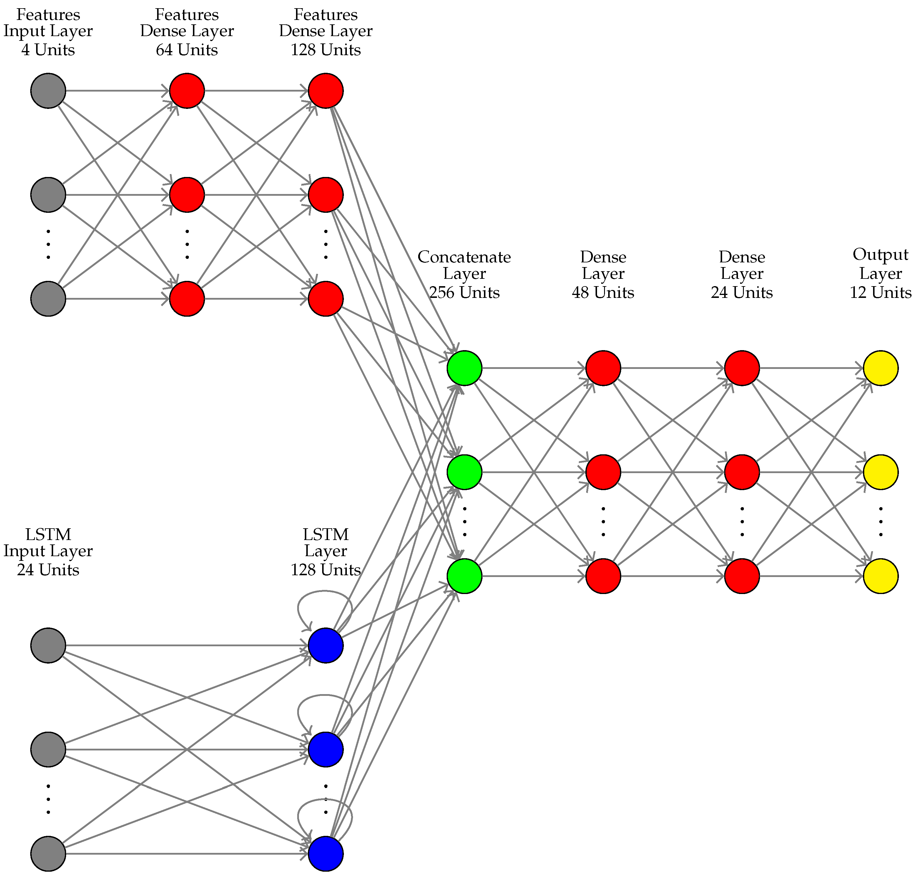
- Combination of two DL architectures to develop a more robust model to detect NTL.
2. Related Work
- Theoretical analysis: Demographic and socioeconomic factors can provide the energy company with information about locations where an NTL may occur more frequently;
- Hardware-based method: It is related to the infrastructure and design of specific measurement devices. For example, integrated circuits (ICs) were installed to detect tampering in energy meters [18] and an additional current transformer (CT) was added to achieve the same result [19]. The disadvantage of this approach is the high costs related to the manufacture, installation and maintenance of these new devices;
- Non-hardware based method: The most widely used method for detecting NTL [17]. Deviations in energy consumption and other electrical quantities, such as voltage and current, occur in an NTL scenario. Using data collected from consumers, a data-oriented/ML method (supervised or unsupervised learning) or a network-oriented method (state estimation or load flow) can be developed to detect whether they are committing any type of fraud.
3. Materials and Methods
3.1. Deep Learning Architectures
3.1.1. MLP
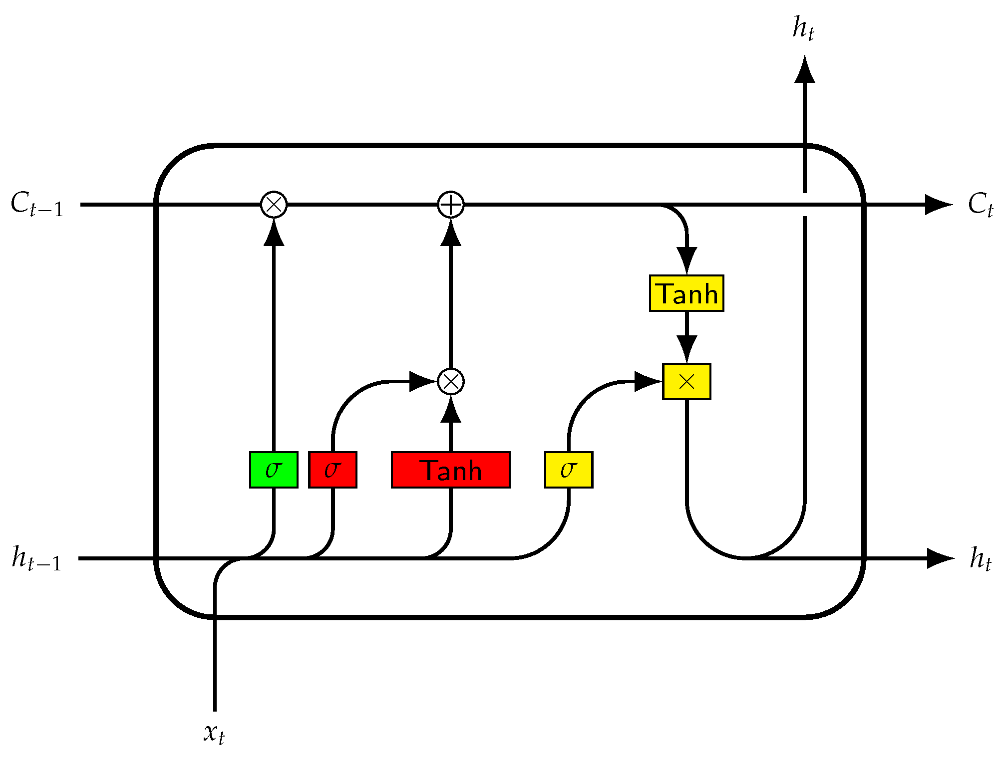
3.1.2. LSTM
3.2. Dataset
- If a half-hourly measurement is not available, the entire day is discarded (missing data case);
- If there is incompatible data, for example, in a single day, a consumer has more than 48 half-hourly measurements, the entire day is also discarded (a possible case of an error in data storage);
- During certain days, some users reported 0 energy consumption. In these cases, if a user has zero energy consumption for more than 1/4 of the day, that entire day is ignored (in case of a possible meter failure).
3.3. Energy Theft Attack Models
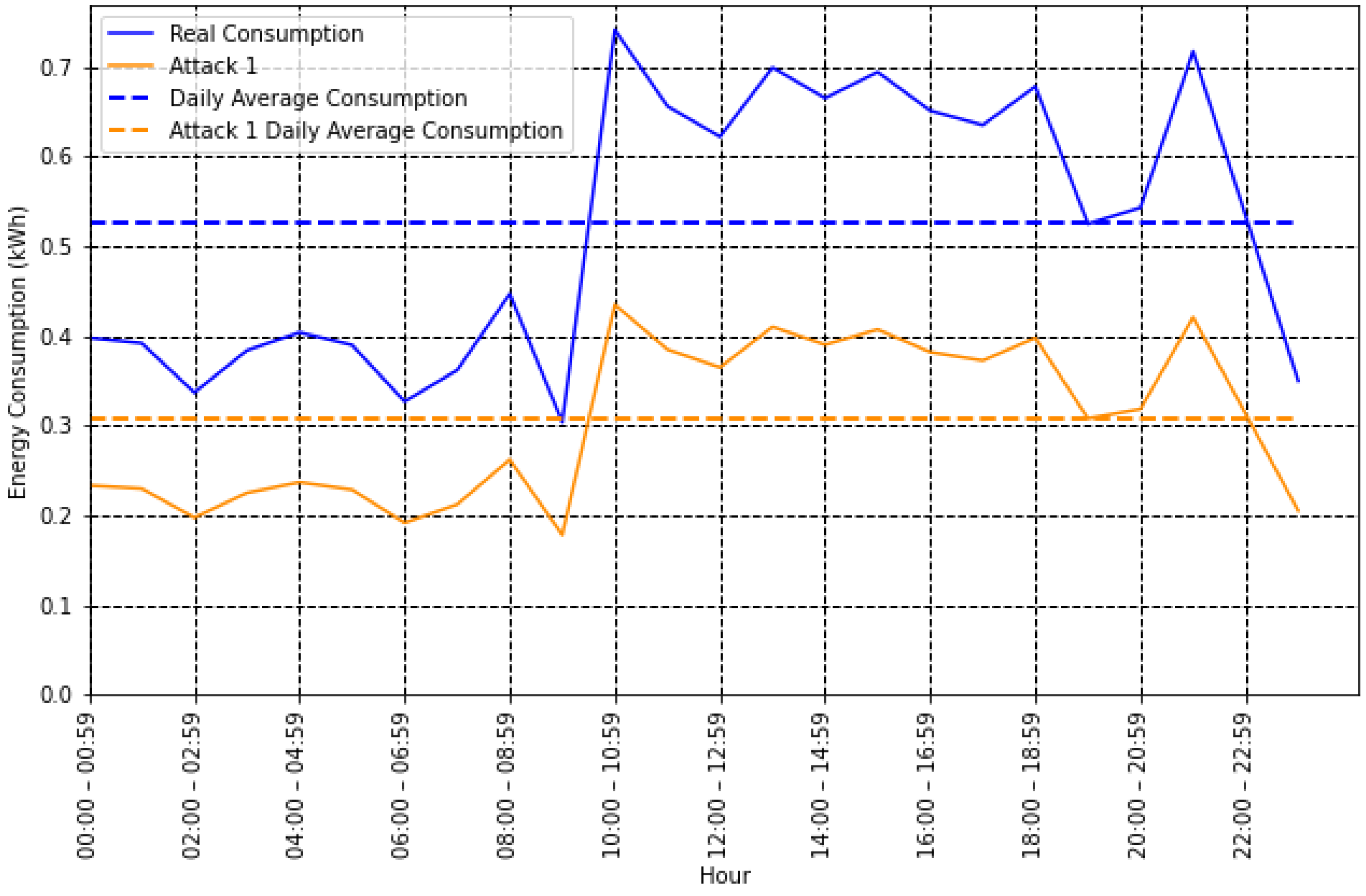
- Attack 1: Each time series is multiplied by a random value , between 0.1 and 0.9 that reduces energy consumption:
- Attack 2: Each smart meter reports 0 while the attack occurs (complete bypass). and represent the start and end times of the attack, respectively. In this work, unless otherwise indicated, all attacks that occur during a period start randomly between 08:00:00 and 16:00:00 and the last 4 h, that is, :
- Attack 3: This attack is similar to Attack 1, but instead of multiplying the whole time series by a random value, the measurements in the time series at each time t are multiplied by a different random value, , between 0.1 and 0.9:
- Attack 4: Similar to Attack 2, but instead of completely bypassing the meter, a partial bypass occurs:
- Attack 5: Actual consumption is replaced by the product between average consumption and different random values:
- Attack 6: A cut-off point, , is selected. A measurement in a time series is replaced by the cut-off point if it is greater than it. The selected point is a random value between 120% and 130% of the average energy consumption, i.e., :
- Attack 7: A cut-off point, , is selected. The maximum value between 0 and the difference between energy consumption and the cut-off point is considered:
- Attack 8: Unlike other attacks, this one does not simulate a sudden drop in energy consumption, but rather the drop occurs linearly over time until the maximum attack intensity. This gradual decay is controlled by the rate of variation in the attack intensity, that is, the slope s:where , and .
- Attack 9: Each energy consumption time series is replaced by its average value:
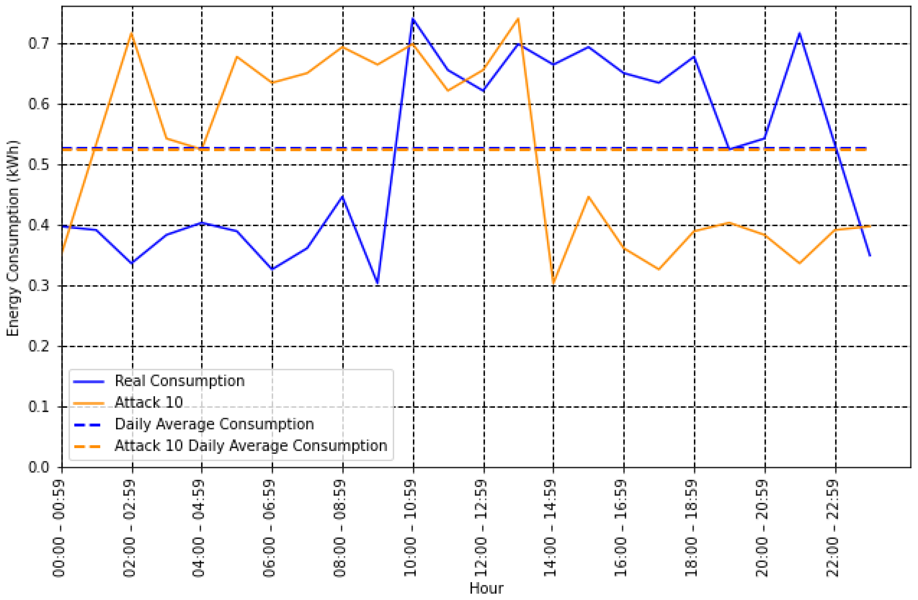
- Attack 10: The energy consumption pattern reverses over time. Attacks of this type occur in situations where the price of energy is different throughout the day. For example, a user who consumes more electricity and has a higher energy tariff at the end of the day, when reversing their pattern, will have a reduced energy bill:
- Attack 11: Another attack that aims to take advantage of different energy rates throughout the day. Consumption is reduced only at a certain interval (peak hours, when the tariff is high) and redistributed throughout the day (when the tariff is lower). This way, the customer’s total consumption remains the same throughout the day:Here is the reduction factor, and for this specific attack, the start time, , happens randomly between 18:00:00 and 20:00:00 and ends randomly at any given time after it has started. Therefore, is the number of hours during the day and is the number of hours during which the attack occurs. is amount of energy that was reduced in the process.
3.4. Features for NTL Detection
- Mean: Most attacks reduce energy consumption, so it is reasonable to assume that the energy consumption value of a fraudulent user is lower than that of an honest user. Therefore, the average value can add valuable information for fraud detection and is calculated as follows:As shown in Figure 2, the mean value of a user who commits type 1 fraud is lower than their real consumption, which could help improve the detection of this type of attack.However, for a type 10 attack, where fraud is committed by reversing the energy consumption pattern, the average value does not change, as shown in Figure 3. Therefore, additional features are needed to improve the classification process.
- Variance: Indicates how far the set of measurements is spread from the average value. Similarly to the average value, the variance of a user who commits fraud will be smaller than the variance of an honest user.
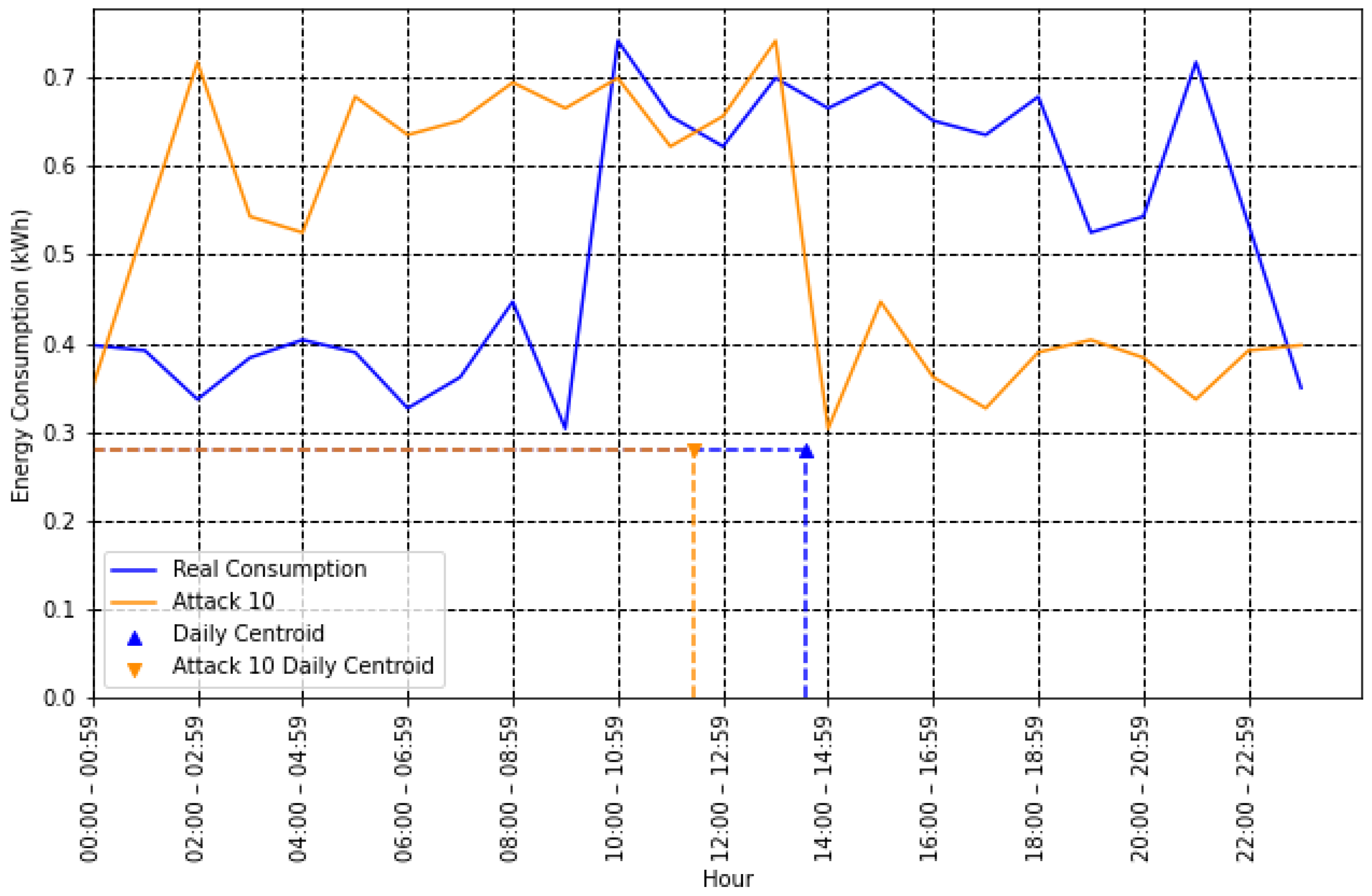
- Centroid (center of mass): Contains information about the time and value of energy consumption. It can potentially help detect an NTL because some attacks tend to occur at specific times of the day, reducing energy consumption only during that interval. The centroid coordinates and can be determined as follows [32]:In Figure 4, the centroids for type 10 attacks are illustrated. The coordinate is essential in this case to help differentiate the honest user from the fraudulent one.
3.5. Developed Models
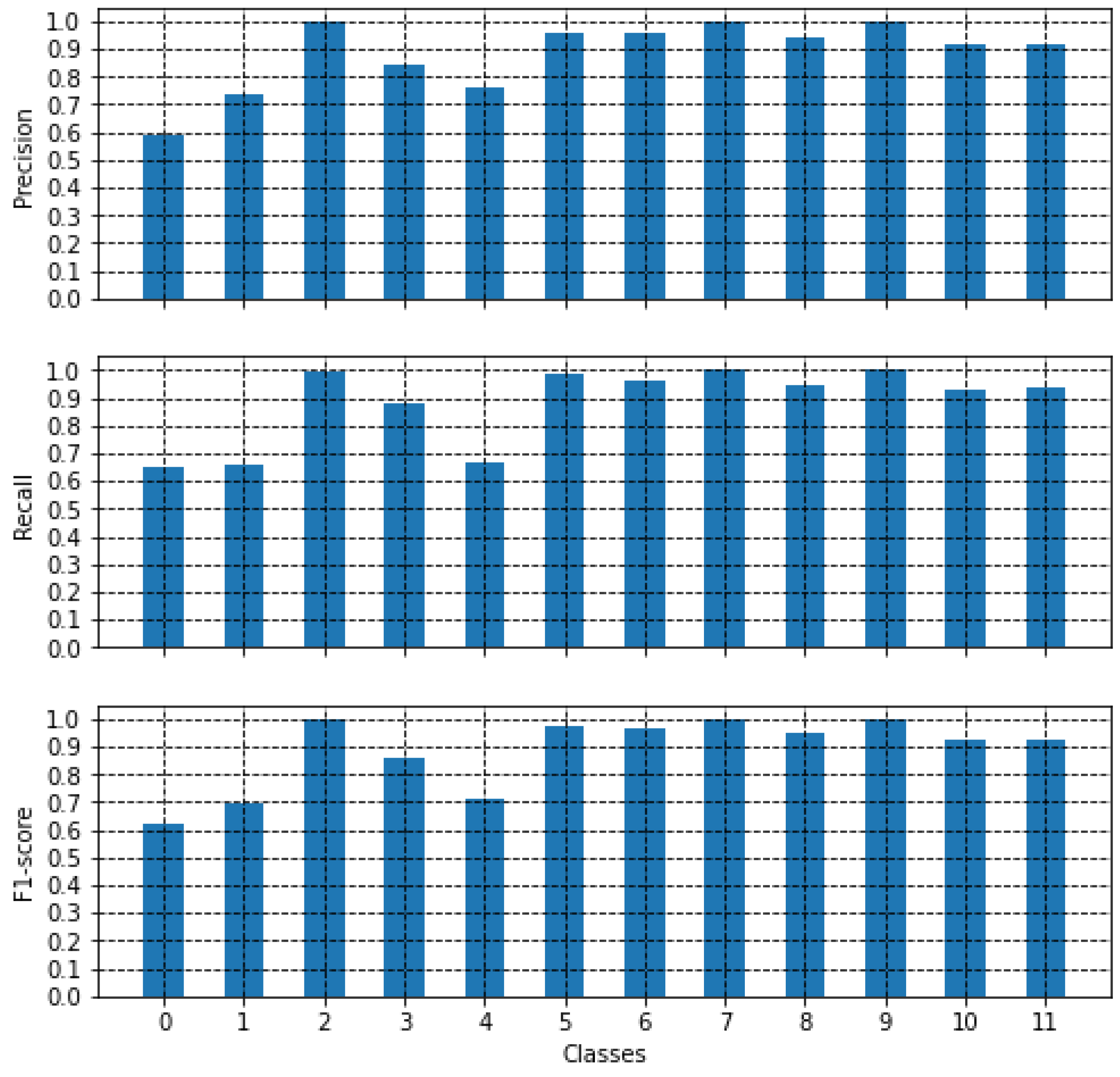
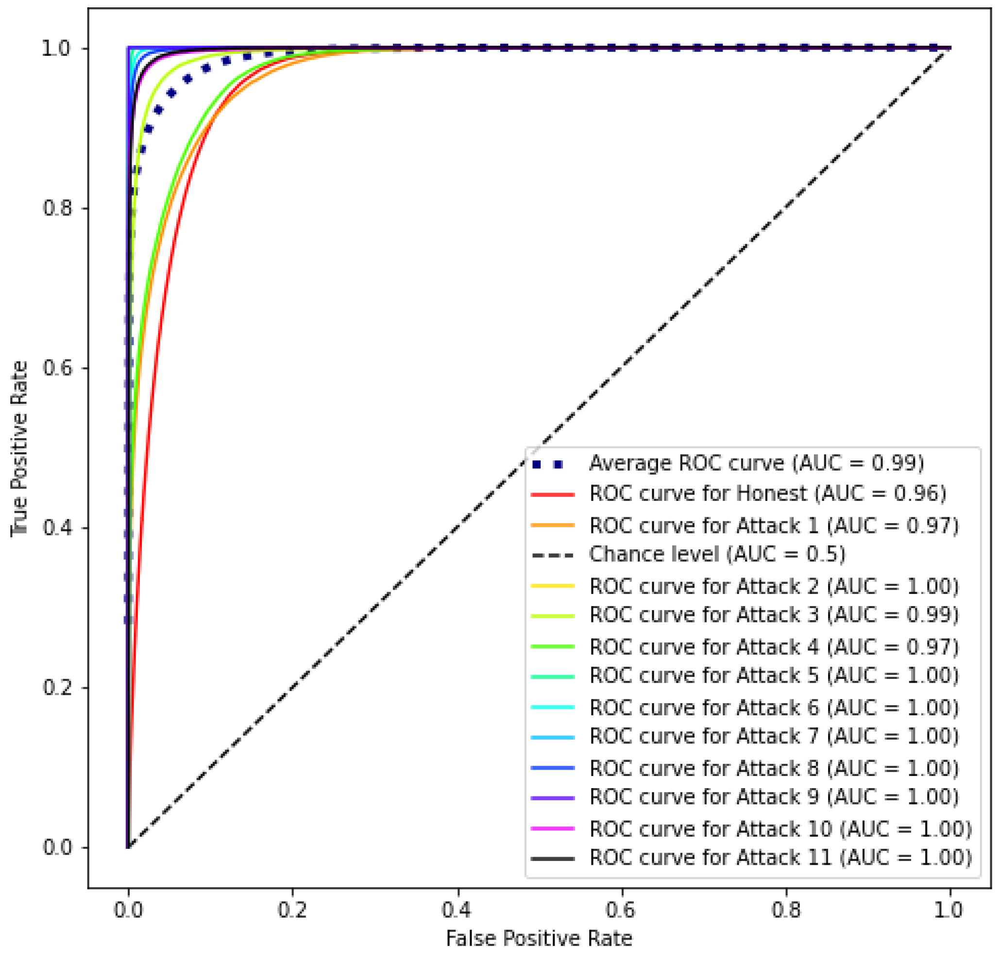
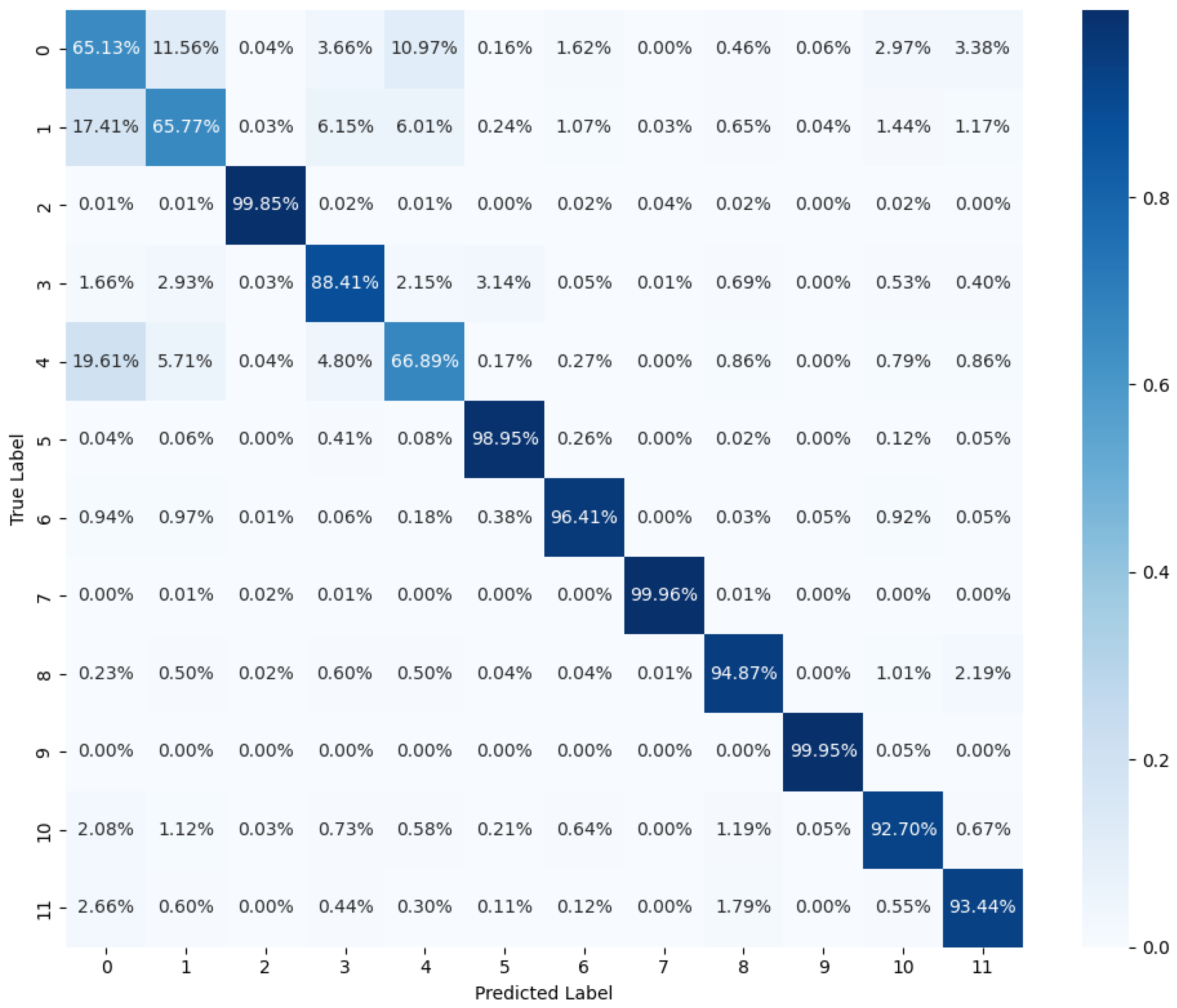
3.6. Classification Metrics
4. Results and Discussion
5. Conclusions
Author Contributions
Funding
Data Availability Statement
Conflicts of Interest
References
- Navani, J.; Sharma, N.; Sapra, S. Technical and Non-Technical Losses in Power System and Its Economic Consequence in Indian Economy. Int. J. Electron. Comput. Sci. Eng. 2012, 1, 757–761. [Google Scholar]
- Smith, T.B. Electricity theft: A comparative analysis. Energy Policy 2004, 32, 2067–2076. [Google Scholar] [CrossRef]
- Northeast Group LLC. Electricity Theft and Non-Technical Losses: Global Markets, Solutions and Vendors. Available online: http://www.northeast-group.com/ (accessed on 20 September 2023).
- McDaniel, P.; McLaughlin, S. Security and Privacy Challenges in the Smart Grid. IEEE Secur. Priv. Mag. 2009, 7, 75–77. [Google Scholar] [CrossRef]
- BC Hydro. Smart Metering & Infrastructure Program Business Case. Available online: https://app.bchydro.com/content/dam/BCHydro/customer-portal/documents/projects/smart-metering/smi-program-business-case.pdf (accessed on 20 September 2023).
- de Souza Savian, F.; Mairesse Siluk, J.C.; Bisognin Garlet, T.; Moraes do Nascimento, F.; Renes Pinheiro, J. Non-technical losses in electricity distribution: A bibliometric analysis. IEEE Lat. Am. Trans. 2021, 19, 359–368. [Google Scholar] [CrossRef]
- ANEEL. Perdas de Energia Elétrica na Distribuição. Available online: https://portalrelatorios.aneel.gov.br/luznatarifa/perdasenergias (accessed on 20 September 2023).
- de Oliveira Ventura, L.; Melo, J.D.; Padilha-Feltrin, A.; Fernández-Gutiérrez, J.P.; Sánchez Zuleta, C.C.; Piedrahita Escobar, C.C. A new way for comparing solutions to non-technical electricity losses in South America. Util. Policy 2020, 67, 101113. [Google Scholar] [CrossRef]
- Olaoluwa, O.G. Electricity Theft and Power Quality in Nigeria. Int. J. Eng. Res. Technol. 2017, 6, 1180–1184. [Google Scholar]
- Wang, W.; Lu, Z. Cyber security in the Smart Grid: Survey and challenges. Comput. Netw. 2013, 57, 1344–1371. [Google Scholar] [CrossRef]
- Jokar, P.; Arianpoo, N.; Leung, V.C.M. Electricity Theft Detection in AMI using customers’ consumption patterns. IEEE Trans. Smart Grid 2016, 7, 216–226. [Google Scholar] [CrossRef]
- Mrabet, Z.E.; Kaabouch, N.; Ghazi, H.E.; Ghazi, H.E. Cyber-security in smart grid: Survey and challenges. Comput. Electr. Eng. 2018, 67, 469–482. [Google Scholar] [CrossRef]
- Morgoev, I.D.; Dzgoev, A.E.; Kuzina, A.V. Algorithm for Operational Detection of Abnormally Low Electricity Consumption in Distribution. In Proceedings of the Advances in Automation V, Sochi, Russia, 10–16 September 2023; Radionov, A.A., Gasiyarov, V.R., Eds.; Springer Nature: Cham, Switzerland, 2024; pp. 37–49. [Google Scholar]
- Nizar, A.H.; Dong, Z.Y.; Jalaluddin, M.; Raffles, M.J. Load Profiling Method in Detecting non-Technical Loss Activities in a Power Utility. In Proceedings of the 2006 IEEE International Power and Energy Conference, Putra Jaya, Malaysia, 28–29 November 2006; pp. 82–87. [Google Scholar] [CrossRef]
- Nagi, J.; Yap, K.S.; Tiong, S.K.; Ahmed, S.K.; Mohamad, M. Nontechnical Loss Detection for Metered Customers in Power Utility Using Support Vector Machines. IEEE Trans. Power Deliv. 2010, 25, 1162–1171. [Google Scholar] [CrossRef]
- Saeed, M.S.; Mustafa, M.W.; Hamadneh, N.N.; Alshammari, N.A.; Sheikh, U.U.; Jumani, T.A.; Khalid, S.B.A.; Khan, I. Detection of Non-Technical Losses in Power Utilities—A Comprehensive Systematic Review. Energies 2020, 13, 4727. [Google Scholar] [CrossRef]
- Viegas, J.L.; Esteves, P.R.; Melício, R.; Mendes, V.; Vieira, S.M. Solutions for detection of non-technical losses in the electricity grid: A review. Renew. Sustain. Energy Rev. 2017, 80, 1256–1268. [Google Scholar] [CrossRef]
- Ngamchuen, S.; Pirak, C. Smart anti-tampering algorithm design for single phase smart meter applied to AMI systems. In Proceedings of the 2013 10th International Conference on Electrical Engineering/Electronics, Computer, Telecommunications and Information Technology, Krabi, Thailand, 15–17 May 2013; pp. 1–6. [Google Scholar] [CrossRef]
- Dey, H.S.; ul Mamun, M.; Shahadat, M.; Ahamed, A.; Ahamed, S.U.; Arefin, K.S. Design and Implementation of a Novel Protection Device to Prevent Tampering and Electricity Theft in Commercial Energy Meters. J. Comput. Inf. Technol. 2010, 1, 88–94. [Google Scholar]
- Ramos, C.C.; Souza, A.N.; Chiachia, G.; Falcão, A.X.; Papa, J.P. A novel algorithm for feature selection using Harmony Search and its application for non-technical losses detection. Comput. Electr. Eng. 2011, 37, 886–894. [Google Scholar] [CrossRef]
- Zanetti, M.; Jamhour, E.; Pellenz, M.; Penna, M.; Zambenedetti, V.; Chueiri, I. A Tunable Fraud Detection System for Advanced Metering Infrastructure Using Short-Lived Patterns. IEEE Trans. Smart Grid 2019, 10, 830–840. [Google Scholar] [CrossRef]
- Zheng, Z.; Yang, Y.; Niu, X.; Dai, H.N.; Zhou, Y. Wide and Deep Convolutional Neural Networks for Electricity-Theft Detection to Secure Smart Grids. IEEE Trans. Ind. Inform. 2018, 14, 1606–1615. [Google Scholar] [CrossRef]
- Messinis, G.M.; Rigas, A.E.; Hatziargyriou, N.D. A Hybrid Method for Non-Technical Loss Detection in Smart Distribution Grids. IEEE Trans. Smart Grid 2019, 10, 6080–6091. [Google Scholar] [CrossRef]
- Domingues, I.; Amorim, J.P.; Abreu, P.H.; Duarte, H.; Santos, J. Evaluation of Oversampling Data Balancing Techniques in the Context of Ordinal Classification. In Proceedings of the 2018 International Joint Conference on Neural Networks (IJCNN), Rio de Janeiro, Brazil, 8–13 July 2018; pp. 1–8. [Google Scholar] [CrossRef]
- Khan, Z.A.; Adil, M.; Javaid, N.; Saqib, M.N.; Shafiq, M.; Choi, J.G. Electricity Theft Detection Using Supervised Learning Techniques on Smart Meter Data. Sustainability 2020, 12, 8023. [Google Scholar] [CrossRef]
- Gunturi, S.K.; Sarkar, D. Ensemble machine learning models for the detection of energy theft. Electr. Power Syst. Res. 2021, 192, 106904. [Google Scholar] [CrossRef]
- Chuwa, M.G.; Wang, F. A review of non-technical loss attack models and detection methods in the smart grid. Electr. Power Syst. Res. 2021, 199, 107415. [Google Scholar] [CrossRef]
- Guarda, F.G.K.; Hammerschmitt, B.K.; Capeletti, M.B.; Neto, N.K.; dos Santos, L.L.C.; Prade, L.R.; Abaide, A. Non-Hardware-Based Non-Technical Losses Detection Methods: A Review. Energies 2023, 16, 2054. [Google Scholar] [CrossRef]
- Goodfellow, I.; Bengio, Y.; Courville, A. Deep Learning; MIT Press: Cambridge, MA, USA, 2016; Available online: http://www.deeplearningbook.org (accessed on 23 July 2018).
- Haykin, S. Neural Networks and Learning Machines, 3rd ed.; Pearson Education: Hoboken, NJ, USA, 2011. [Google Scholar]
- Commission for Energy Regulation. The Smart Metering Electricity Customer Behaviour Trials. Available online: https://www.ucd.ie/issda/data/commissionforenergyregulationcer/ (accessed on 16 October 2022).
- Strang, G.; Herman, E. Calculus Volume 1; OpenStax: Houston, TX, USA, 2016. [Google Scholar]
- Pham, T. Time–frequency time–space LSTM for robust classification of physiological signals. Sci. Rep. 2021, 11, 6936. [Google Scholar] [CrossRef]


| Model | Number of Inputs | Number of Outputs |
|---|---|---|
| MLP-M1 | 24 | 9 |
| MLP-M2 | 24 | 4 |
| MLP-M3 | 24 | 12 |
| MLP-M4 | 25 | 12 |
| MLP-M5 | 26 | 12 |
| MLP-M6 | 28 | 12 |
| LSTM-M7 | 24 | 12 |
| M8 | 28 | 12 |
| Model | Number of Hidden Layers | Units HL 1 | Units HL 2 |
|---|---|---|---|
| MLP-M1 | 2 | 48 | 18 |
| MLP-M2 | 2 | 48 | 8 |
| MLP-M3 | 2 | 48 | 24 |
| MLP-M4 | 2 | 50 | 24 |
| MLP-M5 | 2 | 52 | 24 |
| MLP-M6 | 2 | 56 | 24 |
| Model | - | ||
|---|---|---|---|
| MLP-M1 | 0.909 | 0.909 | 0.909 |
| MLP-M2 | 0.633 | 0.635 | 0.631 |
| Model | - | ||
|---|---|---|---|
| MLP-M3 | 0.721 | 0.728 | 0.723 |
| MLP-M4 | 0.747 | 0.744 | 0.746 |
| MLP-M5 | 0.759 | 0.766 | 0.761 |
| MLP-M6 | 0.777 | 0.786 | 0.779 |
| Model | - | ||
|---|---|---|---|
| LSTM-M7 | 0.871 | 0.869 | 0.869 |
| M8 | 0.885 | 0.885 | 0.885 |
Disclaimer/Publisher’s Note: The statements, opinions and data contained in all publications are solely those of the individual author(s) and contributor(s) and not of MDPI and/or the editor(s). MDPI and/or the editor(s) disclaim responsibility for any injury to people or property resulting from any ideas, methods, instructions or products referred to in the content. |
© 2024 by the authors. Licensee MDPI, Basel, Switzerland. This article is an open access article distributed under the terms and conditions of the Creative Commons Attribution (CC BY) license (https://creativecommons.org/licenses/by/4.0/).
Share and Cite
Souza, M.A.; Gouveia, H.T.V.; Ferreira, A.A.; de Lima Neta, R.M.; Nóbrega Neto, O.; da Silva Lira, M.M.; Torres, G.L.; de Aquino, R.R.B. Detection of Non-Technical Losses on a Smart Distribution Grid Based on Artificial Intelligence Models. Energies 2024, 17, 1729. https://doi.org/10.3390/en17071729
Souza MA, Gouveia HTV, Ferreira AA, de Lima Neta RM, Nóbrega Neto O, da Silva Lira MM, Torres GL, de Aquino RRB. Detection of Non-Technical Losses on a Smart Distribution Grid Based on Artificial Intelligence Models. Energies. 2024; 17(7):1729. https://doi.org/10.3390/en17071729
Chicago/Turabian StyleSouza, Murilo A., Hugo T. V. Gouveia, Aida A. Ferreira, Regina Maria de Lima Neta, Otoni Nóbrega Neto, Milde Maria da Silva Lira, Geraldo L. Torres, and Ronaldo R. B. de Aquino. 2024. "Detection of Non-Technical Losses on a Smart Distribution Grid Based on Artificial Intelligence Models" Energies 17, no. 7: 1729. https://doi.org/10.3390/en17071729