
Auditing and Analysis of Natural Gas Consumptions in Small- and Medium-Sized Industrial Facilities in the Greater Toronto Area for Energy Conservation Opportunities


Abstract
1. Introduction
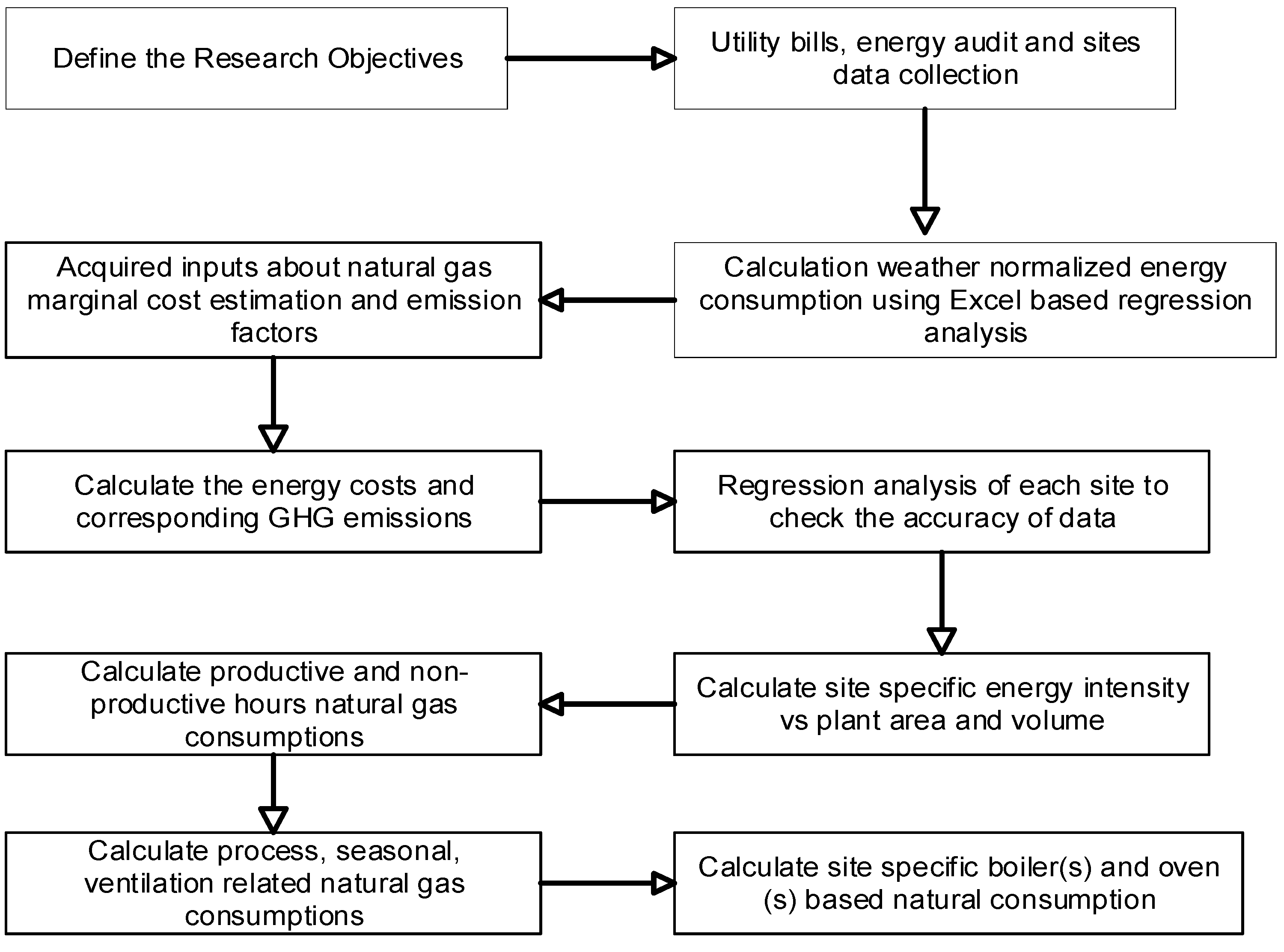
2. Methodology
2.1. Site Selection and Data Collection
2.2. Natural Gas Consumption Analysis
2.3. Productive and Non-Productive Consumption
2.4. Weather Normalized Energy Consumption
NAC = 365 α + δh βh Ho(τh) + δc βc Co(τc)
- α—daily base level consumption;
- βh—daily consumption per heating degree day;
- βc—daily consumption per cooling degree day;
- Ho(τh)—long-term average heating degree days per year;
- Co(τc)—long-term average cooling degree days per year;
- δh—‘1′ for heating only (HO) and “combined heating and cooling” (HC) model, otherwise zero;
- δc—‘1′ for cooling only (CO) and “combined heating and cooling” (HC) model, otherwise zero.
- CFM—ventilation rate;
- τ—reference temperature from the regression analysis;
- ηequipment—thermal efficiency of make-up air unit (%);
- HHVV—higher heating value of natural gas on volume basis;
- —long term average outdoor temperature.
2.5. Marginal Cost of Natural Gas

| Delivery to Customer Breakdown | |
|---|---|
| Amount of gas used per month in cubic meters | Cost in CAD cents per cubic meter (¢/m3) |
| First 500 | 8.1357 |
| Next 1050 | 6.4065 |
| Next 4500 | 5.1958 |
| Next 7000 | 3.10177 |
| Next 15,250 | 4.0721 |
| Over 28,300 | 3.9853 |
| Cost Adjustment Breakdown (CAD) | |
|---|---|
| Gas Supply | 0.9021 ¢/m3 |
| Transportation | 0.1660 ¢/m3 |
| Delivery | –0.2061 ¢/m3 |
| Total Cost Adjustment | 0.8620 ¢/m3 |
| Charge | Rate (¢/m3) (CAD) |
|---|---|
| Gas supply charge | 12.7159 |
| Transportation to Enbridge | 3.15665 |
| Cost adjustment | 0.8620 |
| Delivery to Customer | 3.9853 |
| Total Marginal Cost | 20.72 |
2.6. Greenhouse Gas Emission Factor
3. Results and Discussion
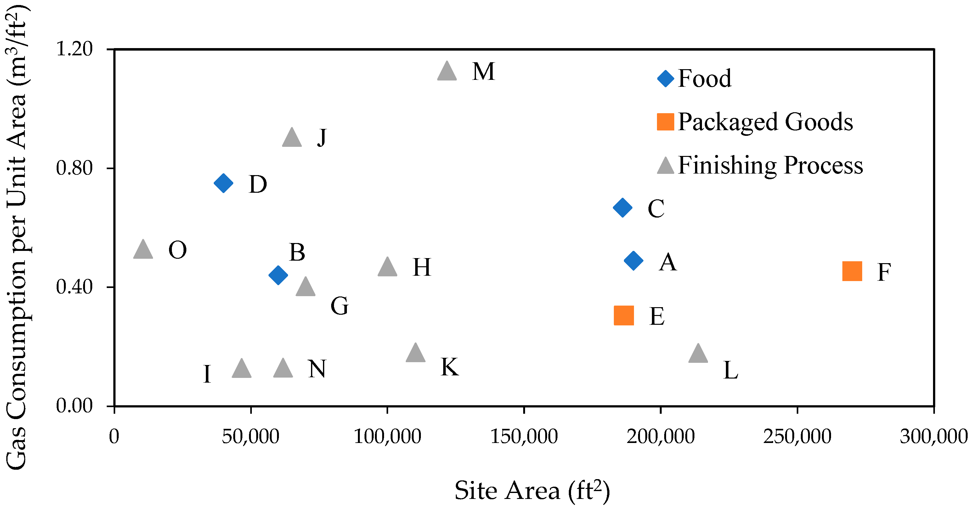
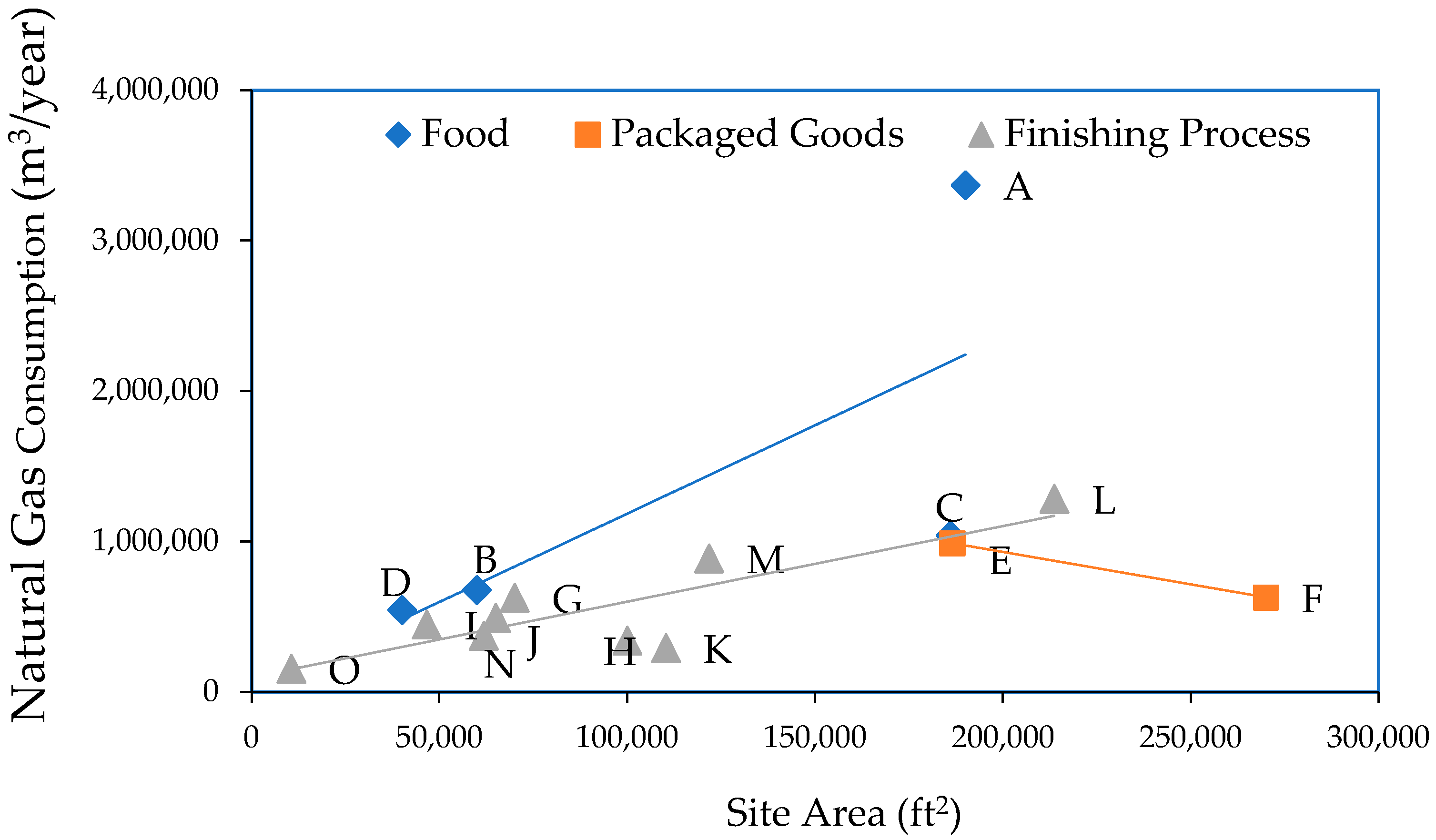
3.1. Natural Gas Consumption
3.1.1. Natural Gas Consumption from the Collected Data
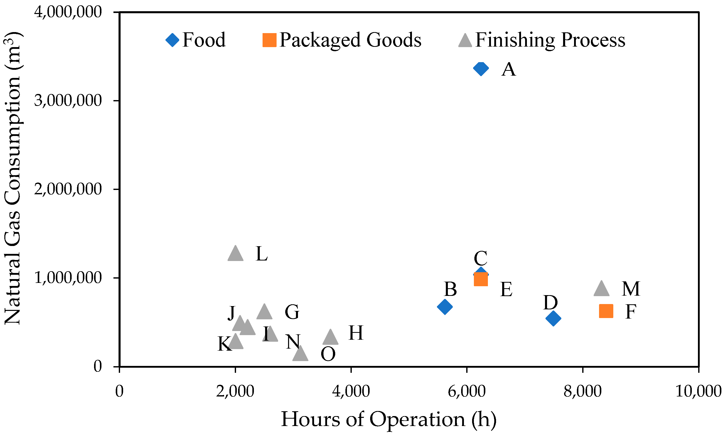
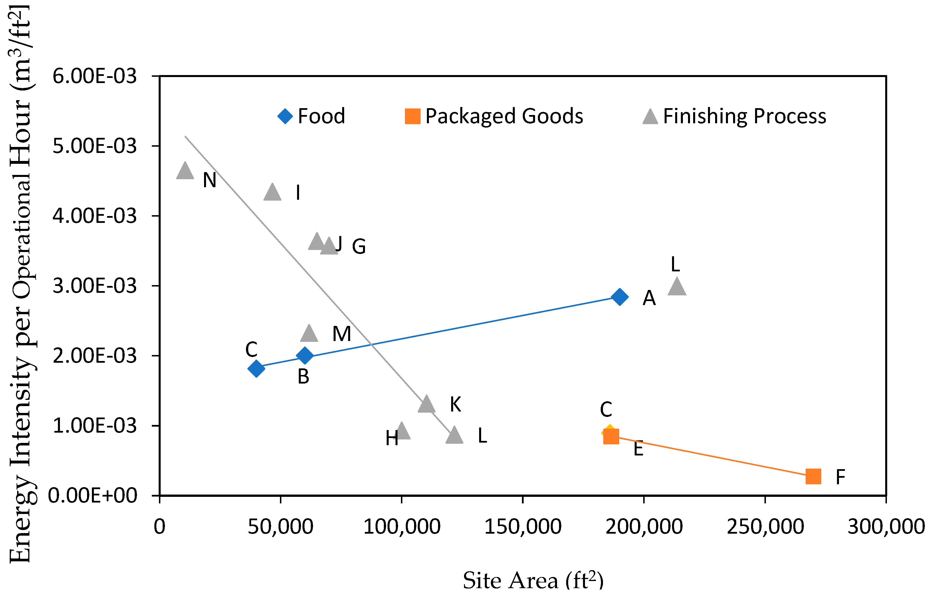
3.1.2. Natural Gas Consumption and Hours of Operation
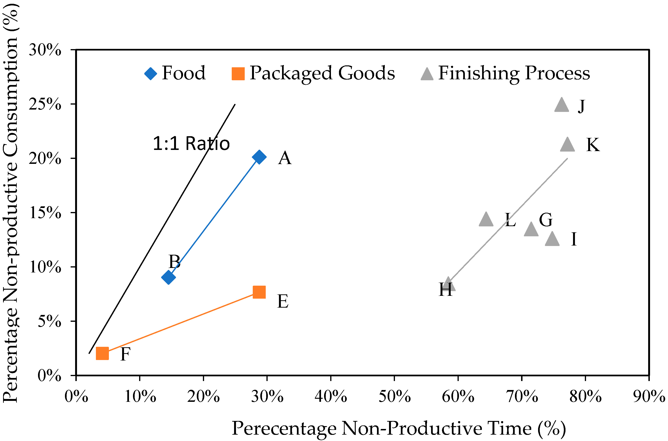
3.1.3. Productive and Non-Productive Natural Gas Consumption
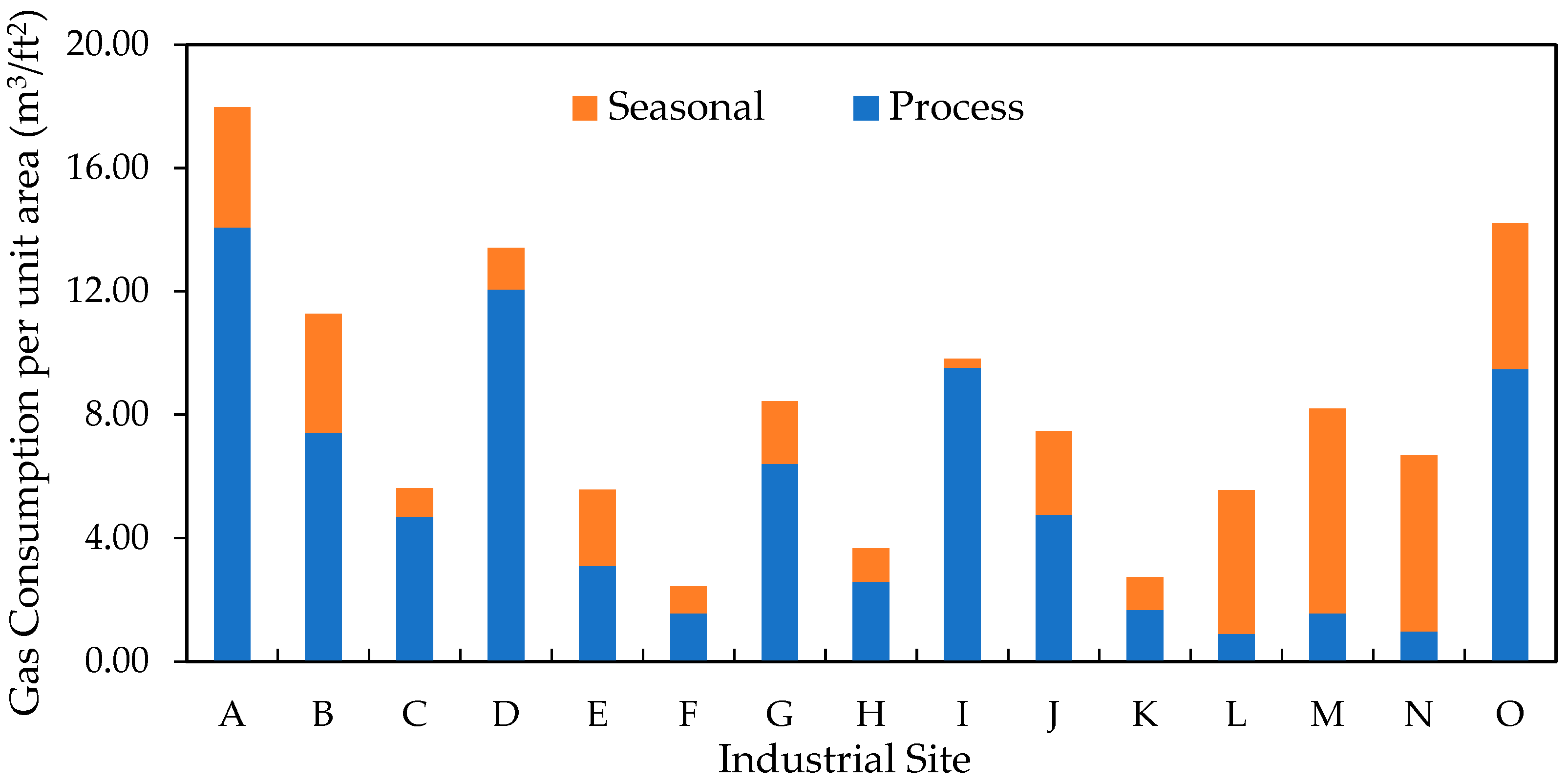
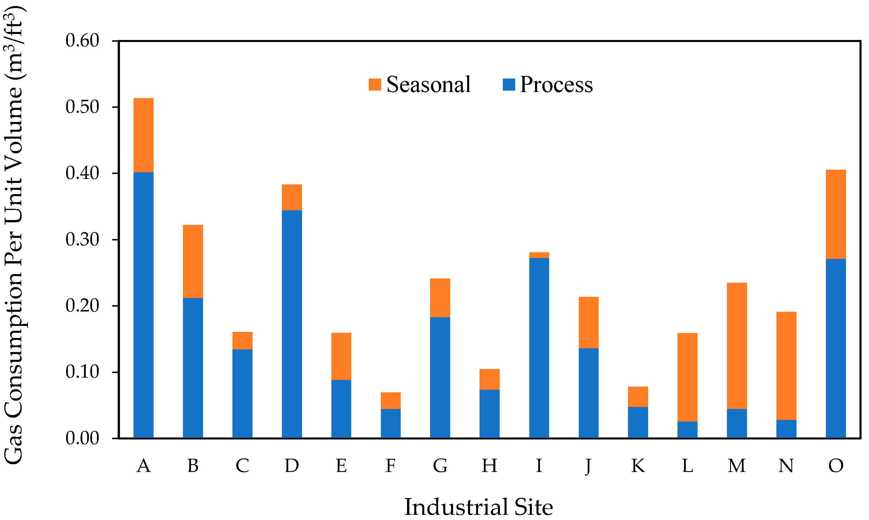
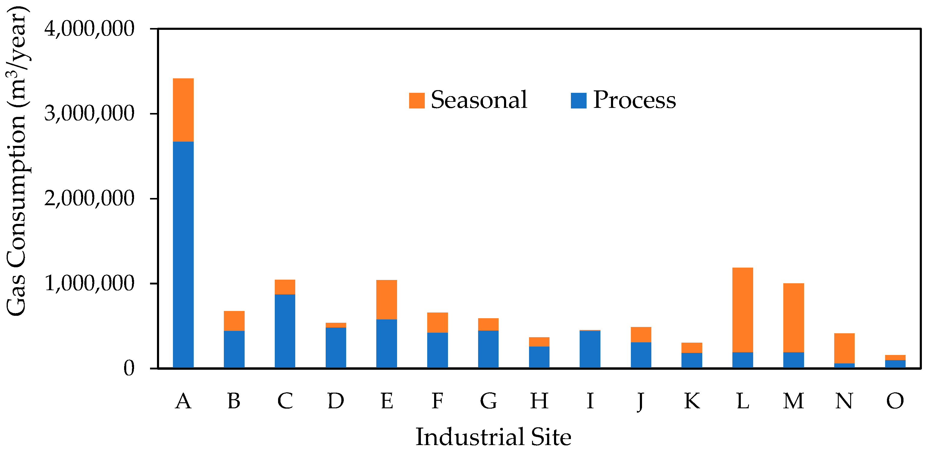
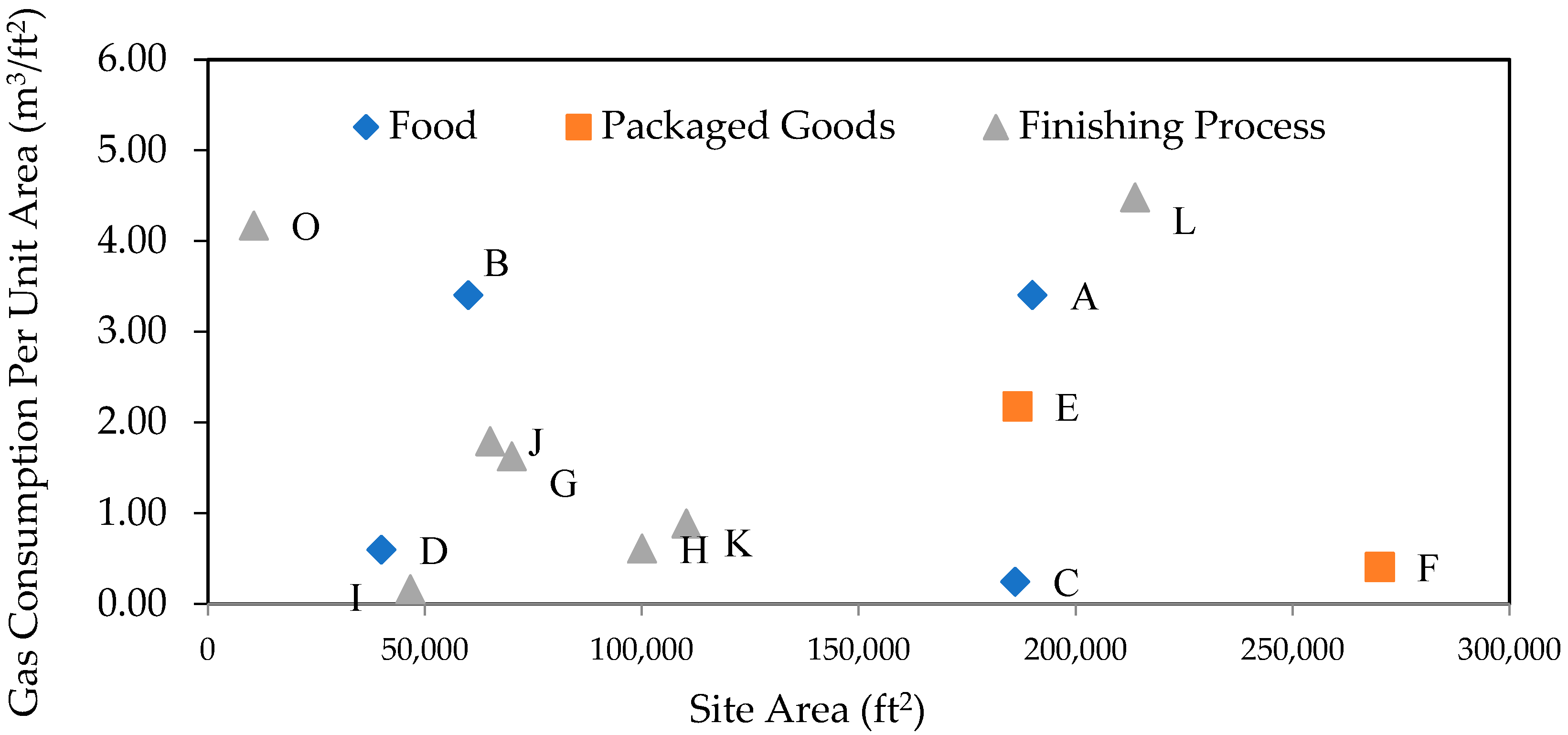
3.1.4. Normalized Natural Gas Consumption
3.2. Major-Gas-Fired Equipment
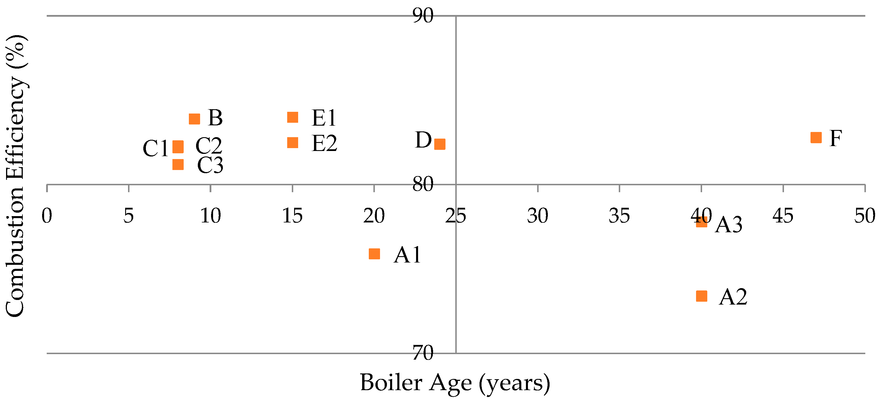
3.2.1. Boiler Performance
3.2.2. Ovens
4. Conclusions
5. Limitation of Study and Further Scope
Author Contributions
Funding
Data Availability Statement
Acknowledgments
Conflicts of Interest
References
- Bataille, C.; Melton, N. Energy efficiency and economic growth: A retrospective CGE analysis for Canada from 2002 to 2012. Energy Econ. 2017, 64, 118–130. [Google Scholar] [CrossRef]
- Bosu, I.; Mahmoud, H.; Hassan, H. Energy audit and management of an industrial site based on energy efficiency, economic, and environmental analysis. Appl. Energy 2023, 333, 120619. [Google Scholar] [CrossRef]
- World SME Forum (WSF). About World SME Forum. 2020. Available online: http://www.worldsmeforum.org/about/ (accessed on 29 March 2024).
- Pansiri, J.; Temtime, Z.T. Assessing managerial skills in SMEs for capacity building. J. Manag. Dev. 2008, 27, 251–260. [Google Scholar] [CrossRef]
- Calogirou, C.; Sørensen, S.Y.; Larsen, P.B.; Pedersen, K.; Kristiansen, K.R.; Mogensen, J.; Alexopoulou, S.; Marie Papageorgiou, M. SMEs and the Environment in the European Union. Planet SA and Danish Technological Institute for European Commission, DG Enterprise and Industry 2010, Brussels. Available online: https://op.europa.eu/en/publication-detail/-/publication/aa507ab8-1a2a-4bf1-86de-5a60d14a3977 (accessed on 30 March 2024).
- Hillary, R. Environmental management systems and the smaller enterprise. J. Clean. Prod. 2004, 12, 561–569. [Google Scholar] [CrossRef]
- McKenzie, R. Canada’s National Partnership Strategy for Industrial Energy Efficiency. In Proceedings of the International Energy Agency, Conference Proceedings—Industrial Energy Efficiency: Policies and Programs, Washington, DC, USA, 26–27 May 1994; Available online: https://www.osti.gov/biblio/20001853 (accessed on 3 February 2015).
- Akan, M.M.; Fung, A.S.; Kumar, R. Process energy analysis and saving opportunities in small and medium size enterprises for cleaner industrial production. J. Clean. Prod. 2019, 233, 43–55. [Google Scholar] [CrossRef]
- Khan, S.A.R.; Sheikh, A.A.; Ahmad, Z. Developing the interconnection between green employee behavior, tax avoidance, green capability, and sustainable performance of SMEs through corporate social responsibility. J. Clean. Prod. 2023, 419, 138236. [Google Scholar] [CrossRef]
- Jago, P. The Canadian Industry Program for Energy Conservation (CIPEC): The dynamics of a 24-year partnership between government and industry. In Proceedings of the 1999 American Council for an Energy-Efficient Economy Summer Study on Energy Efficiency in Industry, Albany, NY, USA, 15–18 June 1999. [Google Scholar]
- Sambor, D.J.; Penn, H.; Jacobson, M.Z. Energy optimization of a food-energy-water microgrid living laboratory in Yukon, Canada. Energy Nexus 2023, 10, 100200. [Google Scholar] [CrossRef]
- Anderson, S.T.; Newell, R.G. Information programs for technology adoption: The case of energy–efficiency audits. Resour. Energy Econ. 2004, 26, 27–50. [Google Scholar] [CrossRef]
- Barbose, G.L.; Goldman, C.A.; Hoffman, I.M.; Billingsley, M. The future of utility customer–funded energy efficiency programs in the USA: Projected spending and savings to 2025. Energy Effic. 2013, 6, 475–493. [Google Scholar] [CrossRef]
- Thollander, P.; Danestig, M.; Rohdin, P. Energy policies for increased industrial energy efficiency: Evaluation of a local energy programme for manufacturing SMEs. Energy Policy 2007, 35, 5774–5783. [Google Scholar] [CrossRef]
- Ahmed, T.; Fung, A.S.; Kumar, R. Energy benchmarking and ventilation related energy saving potentials for SMEs in Greater Toronto Area. J. Clean. Prod. 2020, 246, 118961. [Google Scholar] [CrossRef]
- Boyd, G.A. Motivating Auto Manufacturing Energy Efficiency Through Performance-based Indicators. J. Engines 2006, 115, 284–289. [Google Scholar]
- Government of Canada. Emission Factors and Reference Values. Government of Canada 2023. Available online: https://www.canada.ca/en/environment-climate-change/services/climate-change/pricing-pollution-how-it-will-work/output-based-pricing-system/federal-greenhouse-gas-offset-system/emission-factors-reference-values.html (accessed on 24 December 2023).
- Andersson, E.; Arfwidsson, O.; Thollander, P. Benchmarking energy performance of industrial small and medium-sized enterprises using an energy efficiency index: Results based on an energy audit policy program. J. Clean. Prod. 2018, 182, 883–895. [Google Scholar] [CrossRef]
- Baig, A.A. Analysis of Natural Gas Consumption and Energy Saving Measures for Small and Medium-Sized Industries in the Greater Toronto Area (GTA). Master’s Thesis, Ryerson University, Toronto, ON, Canada, 2014. [Google Scholar]
- Enbridge Gas Distribution Inc. Purchasing Gas from Enbridge. Enbridge Gas Distribution Inc. 2015. Available online: https://www.enbridgegas (accessed on 3 February 2015).
- Rachlin, J.; Fels, M.F.; Socolow, R.H. The Stability of PRISM Estimates. Energy Build. 1986, 9, 149–157. [Google Scholar] [CrossRef]
- ASHRAE. Thermal Environmental Conditions for Human Occupancy. American Society of Heating, Refrigerating and Air Conditioning Engineers. ANSI/ASHRAE 55-2010. Available online: https://www.ashrae.org/technical-resources/bookstore/standard-55-thermal-environmental-conditions-for-human-occupancy (accessed on 3 February 2015).
- RETScreen. Natural Resources Canada. Available online: https://www.nrcan.gc.ca/energy/software-tools/7465 (accessed on 3 February 2015).
- Energy Efficiency and Renewable Energy Software Tools, U.S Department of Energy. Available online: https://www.energy.gov/eere/amo/software-tools (accessed on 3 February 2015).
- Fels, M.F. PRISM: An introduction. Energy Build. 1986, 9, 5–18. [Google Scholar] [CrossRef]
- Fels, M.; Kissock, K.; Marean, M.; Reynolds, C. Description of PRISM® (Advanced Version 1.0)—Users’ Guide; Center for Energy and Environmental Studies; Princeton University: Princeton, NJ, USA, 1995. [Google Scholar]
- Climate Data and Information Archive. Daily Data Report. Retrieved from Environment Canada. Available online: https://climate.weather.gc.ca/historical_data/search_historic_data_e.html (accessed on 3 February 2015).
- Enbridge Gas, Commercial and Industrial. Available online: https://www.enbridgegas.com/business-industrial (accessed on 1 January 2014).


| Monthly Charges | Monthly Rates 1 January 2014 |
|---|---|
| Customer charge | CAD 70 |
| Gas supply charge | CAD 0.127159/m3 |
| Delivery to customer | See breakdown in Table 2 |
| Transportation to Enbridge | CAD 0.49665/m3 |
| Site | Type of Industry | Natural Gas Consumption (m3/Year) | Cost (CAD /Year) | GHG Emission (Tonnes CO2/Year) | Site Area (ft2) | Energy Intensity (m3/ft2) |
|---|---|---|---|---|---|---|
| A | Food | 3,369,563 | 759,152 | 6331 | 190,008 | 17.73 |
| B | 676,090 | 152,321 | 1270 | 60,000 | 11.27 | |
| C | 1,040,399 | 234,399 | 1955 | 186,026 | 5.59 | |
| D | 544,200 | 122,607 | 1023 | 40,000 | 13.61 | |
| E | Packaged Goods | 987,794 | 222,547 | 1856 | 186,500 | 5.30 |
| F | 628,339 | 141,563 | 1181 | 270,000 | 2.33 | |
| G | Finishing Process | 625,765 | 140,983 | 1176 | 70,000 | 8.94 |
| H | 340,017 | 76,605 | 639 | 100,000 | 3.40 | |
| I | 447,889 | 100,908 | 842 | 46,609 | 9.61 | |
| J | 492,795 | 111,025 | 926 | 65,000 | 7.58 | |
| K | 290,981 | 65,557 | 547 | 110,270 | 2.64 | |
| L | 1,283,047 | 289,067 | 2411 | 213,668 | 6.00 | |
| M | 886,747 | 199,781 | 1666 | 121,762 | 7.28 | |
| N | 373,955 | 84,251 | 703 | 61,756 | 6.06 | |
| O | 153,529 | 34,590 | 288 | 10,573 | 14.52 |
| Site | Type of Industry | Average Annual Consumption (m3/Year) | Annual Hours of Operation (h/Year) | Energy Per Hour of Operation (m3/h) |
|---|---|---|---|---|
| A | Food | 3,369,563 | 6240 | 540 |
| B | 676,090 | 5616 | 120 | |
| C | 1,040,399 | 6240 | 167 | |
| D | 544,200 | 7488 | 73 | |
| E | Packaged Goods | 987,794 | 6240 | 158 |
| F | 628,339 | 8400 | 75 | |
| G | Finishing Process | 625,765 | 2500 | 250 |
| H | 340,017 | 3640 | 93 | |
| I | 447,889 | 2210 | 203 | |
| J | 492,795 | 2080 | 237 | |
| K | 290,981 | 2000 | 145 | |
| L | 1,283,047 | 2000 | 642 | |
| M | 886,747 | 8320 | 107 | |
| N | 373,955 | 2600 | 144 | |
| O | 153,529 | 3120 | 49 |
| Site | Average Annual Non-Productive Consumption (m3/Year) | Percentage of Annual Consumption (%) | Average Annual Non-Productive Time (h/Year) | Percentage of Total Hours in a Year (%) |
|---|---|---|---|---|
| A | 677,810 | 20 | 2520 | 29 |
| D | 49,166 | 9 | 1272 | 15 |
| E | 75,710 | 8 | 2520 | 29 |
| F | 12,798 | 2 | 360 | 4 |
| G | 844,18 | 13 | 6260 | 71 |
| H | 28,719 | 8 | 5120 | 58 |
| I | 56,490 | 13 | 6550 | 75 |
| J | 123,000 | 25 | 6680 | 76 |
| L | 273,395 | 21 | 6760 | 77 |
| N | 53,885 | 14 | 6160 | 64 |
| Site | Average Productive Time Consumption (m3/Day) | Average Non-Productive Time Consumption (m3/Day) | Non-Productive Consumption as a Percentage of Productive Consumption (%) |
|---|---|---|---|
| A | 10,753 | 6368 | 59 |
| D | 1630 | 806 | 49 |
| E | 2250 | 670 | 30 |
| F | 1768 | 1422 | 72 |
| H | 1239 | 365 | 29 |
| I | 1537 | 620 | 40 |
| J | 1715 | 683 | 40 |
| L | 11,837 | 7139 | 60 |
| N | 1385 | 922 | 70 |
| Site | Normalized Annual Consumption (NAC) | Process Consumption | Seasonal Consumption | Coefficient of Correlation |
|---|---|---|---|---|
| (m3/Year) | (m3/Year) | (m3/Year) | (R2) | |
| A | 3,413,970 | 2,674,165 | 739,805 | 0.696 |
| B | 676,108 | 445,394 | 230,714 | 0.482 |
| C | 1,044,810 | 875,345 | 169,465 | 0.525 |
| D | 536,523 | 482,606 | 53,917 | 0.654 |
| E | 1,040,758 | 577,809 | 462,949 | 0.907 |
| F | 656,815 | 424,035 | 232,780 | 0.676 |
| G | 591,037 | 448,844 | 142,193 | 0.737 |
| H | 366,655 | 258,624 | 108,032 | 0.944 |
| I | 458,033 | 444,432 | 13,601 | 0.097 |
| J | 485,668 | 310,243 | 175,426 | 0.861 |
| K | 302,332 | 184,472 | 117,861 | 0.670 |
| L | 1,187,717 | 192,107 | 995,610 | 0.928 |
| M | 999,810 | 191,412 | 808,398 | 0.898 |
| N | 412,363 | 60,978 | 351,385 | 0.761 |
| O | 150,061 | 100,369 | 49,693 | 0.309 |
| Site | Daily Base Consumption Level (αh) | Consumption per Heating Degree Day (βh) | Reference Temperature (τ) |
|---|---|---|---|
| (m3/Day) | (m3/°C-Day) | (°C) | |
| A | 7377.2 | 189.8 | 16.0 |
| B | 1273 | 28.5 | 26.0 |
| C | 2396.5 | 72 | 9.0 |
| D | 1317.9 | 43.5 | 6.0 |
| E | 1594.3 | 158.1 | 14.2 |
| F | 1076.9 | 79.2 | 16.5 |
| G | 1261.3 | 31.3 | 18.0 |
| H | 713.0 | 48.6 | 10.8 |
| I | 1222.8 | 2.5 | 14.2 |
| J | 825.6 | 50.5 | 17.0 |
| K | 451.2 | 49.2 | 13.5 |
| L | 604.1 | 345.6 | 14.1 |
| M | 489.0 | 308.4 | 12.5 |
| N | 199.0 | 68.9 | 21.5 |
| O | 212.0 | 6.8 | 17.0 |
| Site | Boiler Number | Combustion Efficiency (%) | Fuel–Steam Efficiency (%) |
|---|---|---|---|
| A | 1 | 75.9 | 68.4 |
| 2 | 73.4 | 66.1 | |
| 3 | 77.8 | 71.0 | |
| B | 1 | 83.9 | 81.2 |
| C | 1 | 82.2 | 80.5 |
| 2 | 82.3 | 80.6 | |
| 3 | 81.2 | 79.5 | |
| D | 1 | 82.4 | 78.3 |
| E | 1 | 84.0 | 82.7 |
| 2 | 82.5 | 80.8 | |
| F | 1 | 82.8 | 79.8 |
| Site | Consumption (m3/Year) | Cost (CAD/Year) | Percentage of Annual Consumption (%) |
|---|---|---|---|
| A | 1,288,334 | 290,777 | 38 |
| B | 344,917 | 77,848 | 51 |
| C | 616,255 | 139,089 | 59 |
| D | 152,500 | 344,19 | 28 |
| E | 553,165 | 124,849 | 56 |
| F | 293,835 | 66,319 | 47 |
| Site | Type | Consumption | Cost | Oven Consumption as a Percentage of Annual Consumption | Combined Oven Consumption of Oven as a Percentage of Annual Consumption |
|---|---|---|---|---|---|
| (m3/Year) | (CAD/Year) | (%) | (%) | ||
| A | bake oven | 848,676 | 191,546 | 25 | 25 |
| D | bake oven | 366,000 | 82,606 | 54 | 54 |
| G | dry-off | 121,134 | 27,340 | 19 | 42 |
| cure | 140,804 | 31,780 | 23 | ||
| H | dry-off | 119,317 | 26,930 | 35 | 71 |
| cure | 121,134 | 27,340 | 36 | ||
| I | dry-off | 90,000 | 10,157 | 20 | 42 |
| cure | 100,000 | 11,285 | 22 | ||
| J | dry-off | 90,596 | 20,448 | 18 | 42 |
| cure | 119,509 | 26,973 | 24 | ||
| K | dry-off | 68,143 | 15,380 | 23 | 58 |
| cure | 100,394 | 22,659 | 35 | ||
| L | dry-off | 313,444 | 70,744 | 24 | 46 |
| cure | 288,369 | 65,085 | 22 | ||
| M | dry-off | 221,687 | 50,035 | 25 | 60 |
| cure | 310,361 | 70,049 | 35 | ||
| N | dry-off | 183,365 | 41,385 | 49 | 73 |
| cure | 88,015 | 19,865 | 24 | ||
| O | dry-off | 32,565 | 7350 | 21 | 55 |
| cure | 52,809 | 11,919 | 34 |
Disclaimer/Publisher’s Note: The statements, opinions and data contained in all publications are solely those of the individual author(s) and contributor(s) and not of MDPI and/or the editor(s). MDPI and/or the editor(s) disclaim responsibility for any injury to people or property resulting from any ideas, methods, instructions or products referred to in the content. |
© 2024 by the authors. Licensee MDPI, Basel, Switzerland. This article is an open access article distributed under the terms and conditions of the Creative Commons Attribution (CC BY) license (https://creativecommons.org/licenses/by/4.0/).
Share and Cite
Baig, A.A.; Fung, A.S.; Kumar, R. Auditing and Analysis of Natural Gas Consumptions in Small- and Medium-Sized Industrial Facilities in the Greater Toronto Area for Energy Conservation Opportunities. Energies 2024, 17, 1744. https://doi.org/10.3390/en17071744
Baig AA, Fung AS, Kumar R. Auditing and Analysis of Natural Gas Consumptions in Small- and Medium-Sized Industrial Facilities in the Greater Toronto Area for Energy Conservation Opportunities. Energies. 2024; 17(7):1744. https://doi.org/10.3390/en17071744
Chicago/Turabian StyleBaig, Altamash Ahmad, Alan S. Fung, and Rakesh Kumar. 2024. "Auditing and Analysis of Natural Gas Consumptions in Small- and Medium-Sized Industrial Facilities in the Greater Toronto Area for Energy Conservation Opportunities" Energies 17, no. 7: 1744. https://doi.org/10.3390/en17071744
APA StyleBaig, A. A., Fung, A. S., & Kumar, R. (2024). Auditing and Analysis of Natural Gas Consumptions in Small- and Medium-Sized Industrial Facilities in the Greater Toronto Area for Energy Conservation Opportunities. Energies, 17(7), 1744. https://doi.org/10.3390/en17071744