Cost-Optimal Aggregated Electric Vehicle Flexibility for Demand Response Market Participation by Workplace Electric Vehicle Charging Aggregators

Abstract

In recent years, with the growing number of EV charging stations integrated into the grid, optimizing the aggregated EV load based on individual EV flexibility has drawn aggregators’ attention as a way to regulate the grid and provide grid services, such as day-ahead (DA) demand responses. Due to the forecast uncertainty of EV charging timings and charging energy demands, the actual delivered demand response is usually different from the DA bidding capacity, making it difficult for aggregators to profit from the energy market. This paper presents a two-layer online feedback control algorithm that exploits the EV flexibility with controlled EV charging timings and energy demands. Firstly, the offline model optimizes the EV dispatch considering demand charge management and energy market participation, and secondly, model predictive control is used in the online feedback model, which exploits the aggregated EV flexibility region by reducing the charging energy based on the pre-decided service level for demand response in real time (RT). The proposed algorithm is tested with one year of data for 51 EVs at a workplace charging site. The results show that with a 20% service level reduction in December 2022, the aggregated EV flexibility can be used to compensate for the cost of EV forecast errors and benefit from day-ahead energy market participation by USD 217. The proposed algorithm is proven to be economically practical and profitable.

1. Introduction

Recently, electric vehicles (EVs), which—in aggregation—often are seen as a flexible battery resource, have been gaining popularity. With the rapid growth in EV demand, the impact of the aggregated EV load on the grid has drawn significant attention [1]. Various studies have offered solutions to mitigate the burden of the increasing EV load on the grid. Exploiting the flexibility of the charging/discharging time and location is the most common solution [2,3].

EV flexibility was first quantified by defining a flexibility index of EV aggregated demand (FIEVAD) using the probability of the demand increase in EV charging at each time step. The FIEVAD is bound between zero and one and reflects the extent of randomness of EV charging behavior. With a higher FIEVAD, less of a collective trend is observed, and the flexibility to change the collective behavior is higher [4]. Ref. [5] defined three indicators for EV flexibility: the transferable power (TP) and transferable time (TT) indicate the potential of an EV cluster to respond to demand response signals; the flat wave performance (FWP) indicates the peak shaving ability of the EV cluster. These indicators were applied to analyze different charging behaviors on weekdays and weekends.

Some studies treat EVs as controllable loads in the distribution grid and exploit their demand-side flexibility for distribution services. EVs benefit the distribution grid through demand reduction during peak hours [6,7,8]. Ref. [9] reviewed options for a flexibility service by EVs and discussed the technical and economic requirements. In addition to flexibility services, ref. [10] also discussed ancillary services provided by EVs and reviewed control architectures and state-of-the-art smart chargers.

To include flexibility in control algorithms for EV dispatch, ref. [11] proposed an optimal control method to minimize the cost and maximize the flexibility, defined as the upward and downward power deviation an EV charger can offer. Ref. [12] calculated the positive and negative aggregate EV flexibility based on the maximum amount of energy that can be postponed or consumed ahead of schedule at each time step. The sensitivity of the flexibility time series to different combinations of control strategies, tariffs, and EV battery capacities was studied. As the flexibility time series is time-coupled, when the EV operating point departs from the trajectory calculated at the beginning of the day in real time, the flexibility time series of the rest of the day changes accordingly.

To describe the aggregated flexibility, ref. [13] offered a method to approximate the aggregated flexibility set from the Minkowski sum of individual EV flexibility sets. Since explicitly computing the Minkowski sum is not achievable, the authors instead proposed an inner and outer approximation which can be computed by solving a linear optimization problem which is solvable. Ref. [14] defined the RT flexibility of the aggregated EV load as the frequency regulation capacity assuming ancillary service participation at an EV charging site. A model predictive control algorithm is used for co-optimization of energy dispatch and frequency regulation with a 5 min resolution. Ref. [15] proposed a maximum entropy feedback control algorithm for the aggregator to assess the RT-aggregated EV flexibility and perform online cost minimizations. The algorithm was tested and proved to be more computationally efficient and to result in a lower cost compared to the traditional MPC control algorithm. Ref. [16] proposed a time-decoupled aggregated EV flexibility region, which is the area between two energy trajectories: an upper trajectory, which is the sum of the individual EV charging trajectories that meet the maximum EV battery energy, and a lower trajectory, which is the sum of the individual EV charging trajectories that meet the minimum customer-requested energy. Individual EV trajectories differ both by the timing of EV charging and the ending state of the charge of the EV battery. The aggregated EV flexibility region, in which all operating points are feasible, is bounded from above by the aggregated upper trajectories and bounded from below by the aggregated lower trajectories. Then, the optimal operating trajectory is chosen based on electricity prices. To disaggregate the optimized aggregate EV load, the dumb charging, first-come-first-served principle is applied. The results show that this online feedback scheme of aggregated EV flexibility characterization is effective.

However, there is a lack of studies focusing on a cost-optimal EV scheduling algorithm that exploits the aggregated EV flexibility for DA demand response under forecast uncertainty. For an aggregated EV charging site with DA demand response market participation, the actual demand response capacity delivered in RT is usually different from the DA forecasted bidding capacity due to forecast uncertainty. To profit from the energy market, it is crucial for aggregators to strategically exploit aggregated EV flexibility as a buffer in RT to compensate for the forecast error and match the DA bidding demand response capacity.

In this work, we follow [16] and develop a cost-optimal EV scheduling algorithm which consists of two parts: (1) Offline optimization, in which the EV charging station aggregator considers demand charge management and bids in the day-ahead (DA) demand response market based on the forecasted aggregated EV load and the recent history of EV loads. (2) Online feedback real-time (RT) optimization (note that “real-time” here does not refer to a real-time market, but rather an optimization run during the day to update the DA dispatch), in which the arrival EV plug-in duration and session energy are updated and fed back to the model predictive control scheme every 15 min. The cost-optimal flexibility region is calculated based on defined service levels, which is the minimum acceptable percentage of the session energy requested by the customers. In online feedback optimization, six service levels are simulated, resulting in six scenarios of RT flexibility regions. RT flexibility exists due to (a) flexibility in the timing of charging, as for most EVs, the layover duration exceeds the required charging duration, and (b) reductions in service level. With online feedback control, the RT flexibility compensates for offline forecast errors and maximizes profits in the DA demand response market. Our method is demonstrated with a case study using real-world EV workplace charging data over one year. The results show that larger service level reductions allow for compensation of revenue losses due to offline optimization forecast errors by DA market revenue from reducing the aggregated EV load.

The main contributions and novelty of this work are as follows:

• A cost-optimal online feedback MPC model is proposed for EV charging site aggregators to profit from the DA energy market under forecast uncertainty by exploiting the aggregated EV flexibility in real time;
• A “value-stacked” cost function including multiple objectives is proposed for the aggregator to jointly consider demand charge management, TOU energy costs, DA market revenue, and EV charging service revenue;
• A detailed DA market bidding strategy which allows utilizing real-time aggregated EV flexibility to avoid under-performance during demand reduction is proposed.

The rest of the paper is organized as follows. Section 2 consists of the model structure, including the optimization control scheme (Section 2.1), the DA demand response market bidding strategy (Section 2.3), and the cost-optimal aggregated EV flexibility region calculation (Section 2.4). The simulation results and cost analysis are presented in Section 3. Finally, Section 4 concludes the paper.

2. Materials and Methods

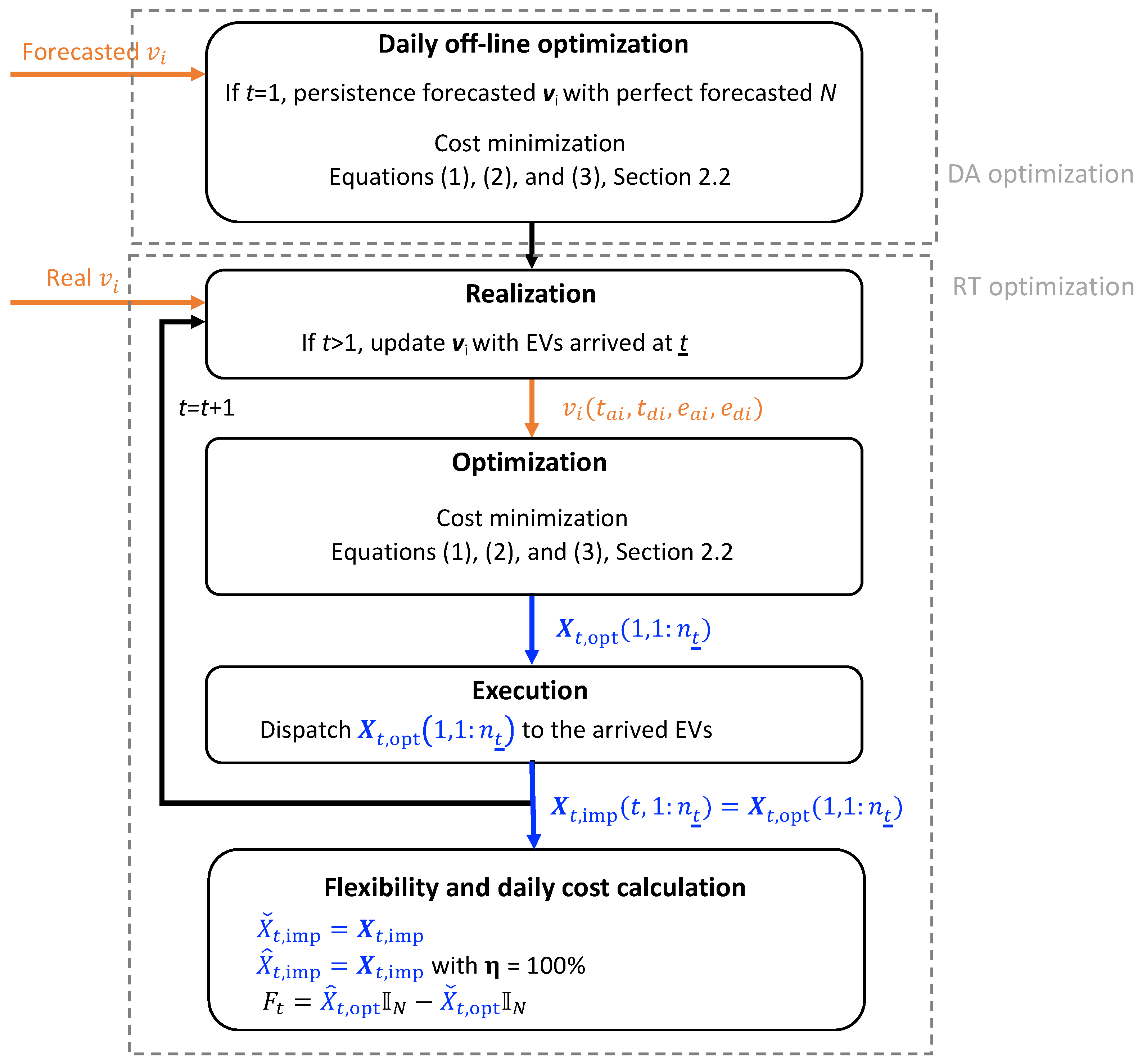
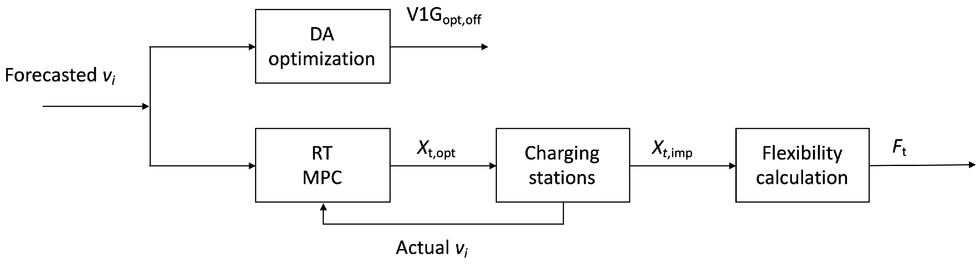
2.1. Offline/Online Optimization Model Overview

Figure 1 presents the model flowchart consisting of DA/offline optimization and RT optimization using a model predictive control (MPC) algorithm. In the optimization, the inputs are a set of forecasted EV arrival and departure times and the energy levels of the EV battery. From the arrival and departure time of EV i, ($t_{\mathrm{ai}}$, $t_{\mathrm{di}}$) (see the nomenclature at the end for all variable definitions), the plug-in duration is calculated. As the model resolution is 15 min, to be conservative, all arrival times are rounded up and departure times are rounded down to the next quarter hour, respectively. From the arrival and requested departure battery energy of EV i, ($e_{\mathrm{ai}}$, $e_{\mathrm{di}}$), the total session energy is calculated. From the charger power rating, the constraint of the maximum interval kWh that can be delivered to EV i during the plug-in duration can be calculated. Note that in reality, without ISO 15118 [17] implementation, the arrival energy is a vehicle property and is unknown and the session energy and departure time are driver inputs and are uncertain. In addition to the algorithm flow chart (Figure 1), a control block diagram is also presented in Figure 2.

In this case study, for the offline/DA optimization model, we assume perfect knowledge of the number of EVs arriving for the following 24 h. In reality, the absolute forecast error for the number of vehicles assuming a persistence forecast is 19% for the year 2022. The smart persistence forecast, which takes the historical data of the previous weekday/weekend (including holidays) day to forecast a weekday/weekend (holiday) day, is used to forecast the plug-in/plug-out times and the session energy of each car a day ahead [18]. These inputs to the MPC are further modified based on the discrepancy of the persistence forecasted and the real number of EVs; the sessions are sorted based on the EV arrival time, and the last n sessions are repeated/excluded if there are n more/less EVs on the current day compared to the forecast.

For the online/RT optimization, the persistence forecasted session energy and departure time of EV i are replaced with the real session energy and departure time of EV i arriving in real time, assuming perfect knowledge of the total session energy and departure time of EV i at the EV arrival time based on driver inputs. We further assume that the actually dispatched session energy in the historical dataset meets 100% of the customer requested session energy; i.e., there are no losses.

The output is an optimal scheduling matrix with rows of 15 min time intervals during the day, columns of N cars of the day, and entries of energy to be charged. For offline optimization, according to the forecasted EV load profile and the baseline, the aggregator can decide the bidding capacity and bidding price for the DA market as further discussed in Section 2.3. For online optimization, the first time step of the output is implemented, and the EV charging results are fed back to the MPC simulation at the next time step, which is further discussed in Section 2.2.

The online feedback process in the RT optimization model is illustrated in Figure 3. The number of time steps in the MPC simulation horizon is H. At time $t=\underline{t}$, the time stamp of the day, both input and output matrices have H time steps, where $H=T-\underline{t}+1$, which cover the time period from the following timestep until the end of the day. The orange input matrix is the constraint of the maximum interval energy capacity of the charger for each EV during its plug-in duration, called the availability matrix, ${\widehat{e}}_t$ (Equation (3)). The orange matrix represents the maximum energy an EV could receive in each time interval. At time $t=\underline{t}$, when $n_{\underline{t}}$ EVs have arrived, the first $n_{\underline{t}}$ columns of the availability matrix are calculated based on the actual arrival and departure times (gray shaded entries), and the rest of the columns are calculated based on the persistence forecasted EV arrival and departure times.

The blue output matrix, $X_{t,\mathrm{opt}}$ (Equation (1)), is the optimal dispatch power at each time interval for each EV. Only the first time step of the first $n_{\underline{t}}$ columns is implemented (the red squared entries). At time $t=\underline{t}+1$, the $(n_{\underline{t}}+1)$th EV arrives, and the $(n_{\underline{t}}+1)$th column of the availability matrix is replaced with the actual values based on the EV arrival and departure times. For the output matrix, only the first time step of the first $n_{\underline{t}+1}$ columns is implemented (red squared entries).

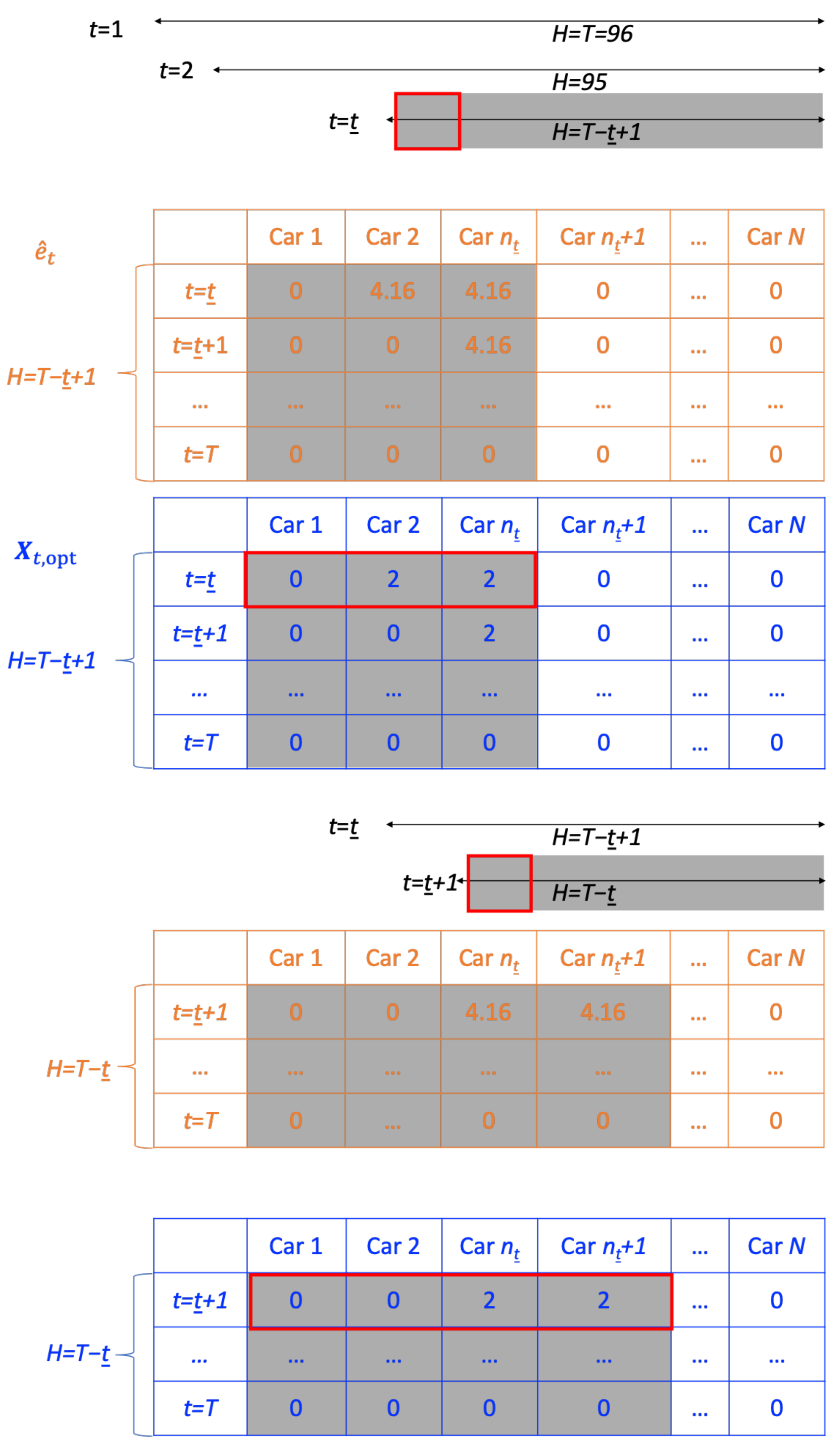
2.2. DA/RT MPC Algorithm

Both DA and RT optimization have the same objective function and constraints. The DA optimization is simulated offline using only the forecasted inputs to determine the DA market bids (see Section 2.3), and no EV dispatch actions are implemented, while the feedback RT optimization includes realization, optimization, and execution stages. For the realization stage, the forecasted inputs are updated with the real arrival/departure time and energy for the EVs that have arrived. For the optimization stage, the MPC model includes the Peak-Demand (PD) charge, Non-Coincident Demand (NCD) charge, Time-of-Use (TOU) energy charge, the EV charging revenue to the aggregator paid by the EV drivers, and the DA energy market revenue. (Demand charges are calculated on a monthly basis. By including demand charges and the demand charge thresholds in the daily optimization, the optimal demand charges are approached without optimizing for a whole month at once [19]. We refer to the first two terms in Equation (1) as the PD/NCD charge of the day.) (Note that currently, according to the CAISO demand response market tariff, the demand response resources must have a minimum load curtailment greater than 500 kW [20], which is one order of magnitude larger than our test setup. However, for this proof of concept, we assume that no minimum capacity is required to participate in the DA demand response market.).

$$\begin{array}{cc}\hfill \underset{X_{t,\mathrm{opt}}}{min}& \left\{\begin{array}{c}{c}_{\mathrm{NCD}}max\{max\left\{X_{t,\mathrm{opt}}{\mathbb{1}}_N\right\}{h}_{t,\mathrm{NCD}}\}+\hfill \\ c_{\mathrm{PD}}max(maxz\left(X_{t,\mathrm{opt}}{\mathbb{1}}_N\right),h_{t,\mathrm{PD}})+\hfill \\ c_{\mathrm{E}}\Delta t\sum _t^T{X}_{t,\mathrm{opt}}{\mathbb{1}}_N-\hfill \\ c_{\mathrm{EV}}\Delta t\sum _t^T{X}_{t,\mathrm{opt}}{\mathbb{1}}_N-\hfill \\ c_{\mathrm{LMP},\mathrm{DA}}\Delta t\sum _{t_1}^{t_2}{z}_{\mathrm{DR}}(X_{t,\mathrm{opt}}{\mathbb{1}}_N-L)\hfill \end{array}\right.\hfill \end{array}$$

(1)

$$\begin{array}{cc}\hfill \mathrm{s}.\mathrm{t}.& {\left({\mathbb{1}}_t{X}_{t,\mathrm{opt}}\right)}_i=\eta (e_{di}-e_{ai})/\Delta t\hfill \end{array}$$

(2)

$$\begin{array}{cc}\hfill & 0<X_{t,\mathrm{opt}}<{\widehat{e}}_t/\Delta t\hfill \end{array}$$

(3)

where $X_{t,\mathrm{opt}}$, a $T-t$ + 1 × N matrix, is the optimal dispatch matrix for all forecasted EVs from time t to T. $X_{t,\mathrm{opt}}$ is bounded between zero and the maximum charger capacity, ${\widehat{e}}_t$, as EV discharging is not considered in this study. ${\mathbb{1}}_N$ is a N× 1 vector with all entries being one. ${\mathbb{1}}_t$ is a 1 ×$T-t$ + 1 vector with all entries being one. z is the filter for peak hours. $c_{\mathrm{NCD}}$, $c_{\mathrm{PD}}$, $c_{\mathrm{E}}$, and $c_{\mathrm{EV}}$ are the NCD rate, PD rate, TOU energy rate, and EV charging site energy rate; $c_{\mathrm{LMP},\mathrm{DA}}$ is the DA demand response price for the offline DA/online RT optimization; $h_{t,\mathrm{NCD}}$ is the highest actual EV load during the prior days of the month till time t; $h_{t,\mathrm{PD}}$ is the highest actual EV load during the peak demand hours during the prior days of the month till time t; L is the baseline reference load for the DA/RT demand response market; $z_{\mathrm{DR}}$ is 0/1 if it is a non-event/event hour; $\eta$ is the service level of both individual and aggregated charging sessions; and ${\widehat{e}}_t$ is the maximum charger energy capacity in a 15 min interval. In the execution stage, only the first time step of the output matrix $X_{t,\mathrm{opt}}$ is implemented, and at time $t=\underline{t}$, when $n_{\underline{t}}$ cars have arrived, the $n_{\underline{t}}$ plugged-in EVs are dispatched accordingly. The dispatched EV energy is updated and sent back to the MPC feedback loop into the realization stage as the updated state for the RT optimization in the next time step.

The service level is decided in the RT optimization and defines what percentage of EV load will be fulfilled. Here, for simplicity, all users agree to the same service level and the service level is fixed for the entire duration of the simulation. Multiple scenarios are simulated with six service levels of 100%, 80%, 60%, 40%, 20%, and 0%. A lower service level, i.e., a larger flexibility region, which is further defined in Section 2.4, provides the aggregator a higher chance to profit from the DA market.

At the end of the daily simulation, for each service level, the implemented dispatch is used to calculate the flexibility region and the corresponding total cost. Note that in an operational setting, the service level could differ at each time step and the forecasted flexibility region should be calculated in RT. However, in this work, for simplicity and to demonstrate the influence of different flexibility regions on forecast error compensation and DR market net revenue, six fixed service levels are simulated and analyzed in retrospect.

2.3. Bidding Strategy and Market Settlement for the DA Demand Response Market

The following bidding strategy is applied: if the forecasted load (at 100% service level) is lower than the baseline load, the aggregator bids at a price equal to the floor price (the floor price is the on-peak and off-peak monthly minimum market clearing prices published by CAISO [21,22]) and the capacity of the difference between the baseline and the forecasted load [19]. (The baseline is calculated on an hourly basis: for the nth hour on a weekday, the baseline hour is the average of the previous ten non-event nth hours of the weekdays. Likewise, for the nth hour on a weekend day or a holiday, the baseline hour is the average of the previous four non-event nth hours of the non-event weekends/holidays.) Note that the actual demand response payouts are based on the market price (not the floor price). Bidding at the floor price is reasonable as the forecasted load is lower than the baseline. That is, the cost of demand “reduction” is zero as there is no loss in EV charging revenue. Details are provided in the results section with a case study.

Mathematically, based on the offline optimization results, the bidding price at hour h, $c_{\mathrm{bid},\mathrm{h}}$, and the bidding capacity at hour h, $p_{\mathrm{bid},\mathrm{h}}$, for the DA market are:

$$\begin{array}{cc}\hfill c_{\mathrm{bid},h}& =\left\{\begin{array}{cc}\underline{c}\hfill & \mathrm{if}{\underline{L}}_h>{\underline{Y}}_{0,h}\hfill \\ \overline{c}\hfill & \mathrm{otherwise}.\hfill \end{array}\right.\hfill \end{array}$$

(4)

$$\begin{array}{cc}\hfill p_{\mathrm{bid},h}& ={\underline{L}}_h-{\underline{Y}}_{0,h}\hfill \end{array}$$

(5)

where $\underline{c}$ is the floor locational marginal price (LMP), and $\overline{c}$ is the ceiling LMP, which is USD 1/kWh (or USD 1/kW, as the DA market has a resolution of one hour) for the CAISO market. $\underline{L}$ is the hourly average of the baseline load L, and ${\underline{L}}_h$ is the hourly baseline load at hour h. $Y_0$ is the DA forecasted load $X_{0,\mathrm{opt}}{\mathbb{1}}_N$, ${\underline{Y}}_0$ is the hourly average of $Y_0$, and ${\underline{Y}}_{0,h}$ is the DA forecasted hourly load at hour h. With this bidding strategy, the aggregator has control over the market participation hours as the floor/ceiling LMP is almost always lower/higher than the DA LMP, and thus a floor/ceiling bidding price almost always results in an event/non-event hour. In Equation (5), the forecasted demand response capacity is the difference between the baseline $L_h$ and the forecasted aggregated EV demand $Y_{0,h}$ as the output from the offline optimization at t = 0. At t = T, the DA demand response settlement contains two parts: the settlement from demand reduction based on the bidding capacity, $S_{\mathrm{DA}}$, and the settlement (penalty) from overperforming (underperforming), $S_{\mathrm{RT}}$. The settlements are calculated based on DA/RT LMP, $c_{\mathrm{LMP},\mathrm{DA}}$, and $c_{\mathrm{LMP},\mathrm{RT}}$, respectively, as

$$\begin{array}{cc}\hfill S_{\mathrm{DA}}& =|\min (L-X_{0,\mathrm{opt}}{\mathbb{1}}_N,L-X_{T,\mathrm{imp}}{\mathbb{1}}_N)|\Delta t{c}_{\mathrm{LMP},\mathrm{DA}},\hfill \end{array}$$

(6)

$$\begin{array}{cc}\hfill S_{\mathrm{RT}}& =(X_{T,\mathrm{imp}}{\mathbb{1}}_N-X_{0,\mathrm{opt}}{\mathbb{1}}_N)\Delta t{c}_{\mathrm{LMP},\mathrm{DA}}.\hfill \end{array}$$

(7)

The total daily settlement is the sum of $S_{\mathrm{DA}}$ and $S_{\mathrm{RT}}$. In both Equations (6) and (7), the time resolution is 15 min. (The raw data of DA and RT LMP are collected on an hourly and 5 min basis, respectively. For consistency, all variables are calculated on a 15 min basis, which matches the dispatch output of the optimization model.) Here, the settlements are calculated based on the baseline of the 100% service level simulation, assuming no service reduction for the baseline days. While the baseline is usually calculated based on the previous ten non-event weekdays or four non-event weekend days [17], here, for simplicity, no historical market participation is assumed and the baseline is calculated based on the prior 10/4 days.

2.4. Aggregated EV Flexibility

The aggregated EV flexibility is defined as the operating region between the maximum and the minimum cost optimal aggregated EV load time series ${\widehat{X}}_{t,\mathrm{opt}}{\mathbb{1}}_N$, ${\check{X}}_{t,\mathrm{opt}}{\mathbb{1}}_N$:

$$\begin{array}{cc}\hfill F_t& ={\widehat{X}}_{t,\mathrm{opt}}{\mathbb{1}}_N-{\check{X}}_{t,\mathrm{opt}}{\mathbb{1}}_N.\hfill \end{array}$$

(8)

where ${\widehat{X}}_{t,\mathrm{opt}}$ is the optimal dispatch matrix based on the 100% session energy satisfaction level, referred to as the service level, and ${\check{X}}_{t,\mathrm{opt}}$ is the optimal dispatch matrix based on the minimal service level. For demonstration purposes, we assume the minimal service level is known and constant throughout the simulation, and six predetermined service levels—100%, 80%, 60%, 40%, 20%, and 0%—are simulated. With this setup, the economic benefit of exploiting the flexibility region is discussed based on the cost optimal dispatch results for each service level, and the impact of service level reduction in demand response market revenue is analyzed.

In real market operation, the aggregator would navigate the conflicting objectives of satisfying the users’ energy demand and maximizing demand response market revenue. If the demand response market prices are unattractive, i.e., the DA LMP is smaller than the net EV charging revenue (the difference between the TOU energy rate paid to the utility and the EV charging rate paid by the EV users), then the aggregator would operate at 100% service level to maximize charging station revenue (and utilization). If the demand response market prices are attractive, then the aggregator would attempt to reduce the service level as much as possible. But there are limits to reducing the service level without risking customer dissatisfaction. In practice, the aggregator could either guarantee a certain service level (e.g., 50%) to all users in their terms and conditions and then freely operate between that service level and 100%. Alternatively, the aggregator could design a market that allows users to communicate their desired charging energy and flexibility at certain remuneration levels. Then, the aggregator could optimize service levels around the user flexibility and price elasticity.

However, note that both of these situations require the aggregator to know the state of charge of the battery upon arrival. Unfortunately, at present, most aggregators do not know the EV battery’s state of charge. The ISO 15118 standard [17] is designed to change that by allowing bidirectional communication between the EV and the charging station. Without this, operators would have to rely on driver communications, e.g., through a mobile application, which are notoriously inaccurate and subject to driver manipulation. For example, the drivers could overstate their energy demand only to get paid for the operator not being able to meet it.

In summary, our assumptions are as follows: (1) The optimization input is based on persistence forecasted EV loads, assuming perfect knowledge of the number of EVs. (2) The optimization input is updated in real time based on the EV arrival/departure energy level and arrival/departure time, which are assumed to be known at the EV arrival time. (3) For the bidding strategy, if the forecasted load is lower than the baseline, we assume that the cost of demand (service) reduction is negligible.

3. Results

3.1. Data and Algorithm

The algorithm was implemented in Python (version 3.10) using the cvxpy solver. The runtime for 1 year of charging dispatch is 2.5 h on an Intel Core i7-4790 CPU at 3.60 GHz, 32.0 GB.

The model was tested with PowerFlex EV charging data from 2022 at the UC San Diego campus with 5 Tesla chargers (with a maximum power capacity of 10.3 kW) and 46 AeroVironment/Webasto DX chargers (with a maximum power capacity of 6.7 kW). The chargers are located at Athena garage and Gilman parking structure on UC San Diego campus. The Gilman parking structure presents a typical workplace charging site, serving staff, faculty, and students at nearby office buildings, labs, and classrooms. The Athena garage serves medical facilities and experiences different charging profiles due to the 12 h shifts of many medical workers and shorter-duration patient and visitor traffic. A total of 502,023 sessions were recorded in 2022.

The utility tariffs are as follows: $c_{\mathrm{NCD}}$, $c_{\mathrm{PD}}$, $c_{\mathrm{E}}$ [23], and $c_{\mathrm{EV}}$ are USD 24.48/kW and USD 28.92/kW in summer; USD 19.23/kW in winter; USD 0.107/kWh for off-peak hours and USD 0.126/kWh for peak hours; and USD 0.150/kWh, respectively. The threshold, $h_{\mathrm{NCD}}$ ($h_{\mathrm{PD}}$), is the highest actual EV load up to time t (during peak demand hours) of the month. The DA and RT market prices are the DA and interval locational marginal prices at UC San Diego obtained from CAISO OASIS [24].

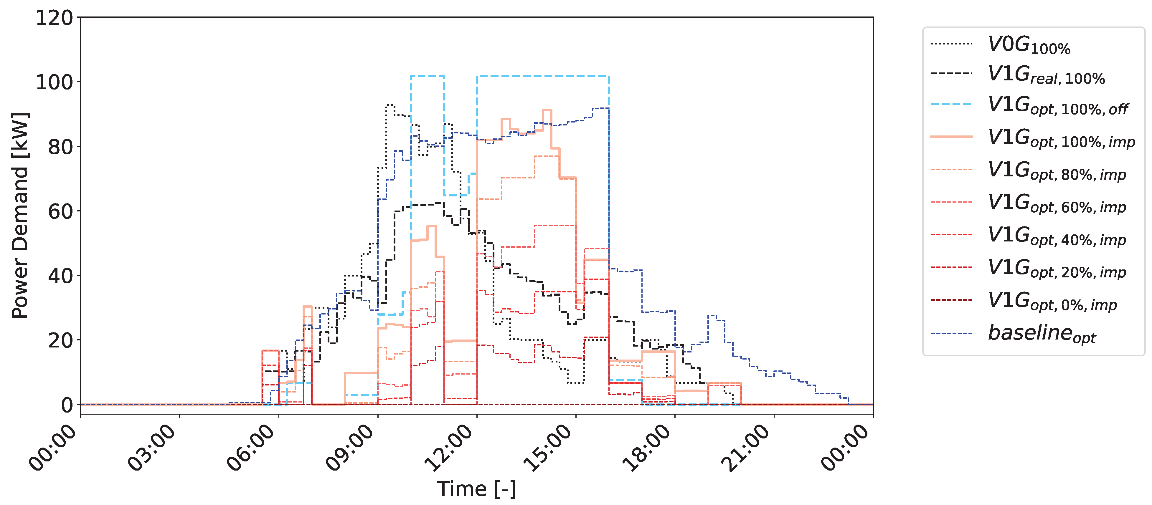
3.2. Daily Profile on 7 December 2022

3.2.1. EV Load and Demand Charges

Figure 4 shows the actual and simulated aggregated EV loads with different control schemes and different service levels on 7 December 2022. The simulated (uncontrolled) dumb charging, with 100% service level, is denoted as V0G_100% (dotted black); the actual PowerFlex controlled, 100% service level load profile of the day is denoted as V1G_real,100% (dashed black). PowerFlex operates chargers based on [25], but since actual site demand charges are not assessed only by the EV charging load, the optimization function differs and the optimization performance in this paper does not reflect the skill of the PowerFlex algorithm. The smart persistence forecasted offline optimal load with 100% service level, as the output of the DA optimization, also referred to as the forecasted optimal load, is denoted as V1G_opt,100%,off (dashed light blue). The baseline_opt (dashed blue) is the average of the V1G optimal implemented load over the previous 10 weekdays (in the simulations) with 100% service level. We assume market participation during hours when the baseline_opt is higher than the forecasted optimal load. Baseline_opt is referred to as the dispatch baseline in the rest of the paper.

Due to forecast errors, the implemented optimal load with 100% service level, V1G_opt,100%,imp (solid light red line), does not match the forecasted optimal load trajectory, V1G_opt,100%,off. V0G_100%, V1G_real,100%, and V1G_opt,100%,imp are the loads controlled by three different schemes, i.e., simulated dumb charging, real PowerFlex-controlled charging, and the simulated cost optimal MPC proposed in this study, respectively. With the cost optimal control, demand charge management is conducted by shaving the peak load based on the thresholds (104 kW for NCD and 41 kW for PD based on EV energy demand between 1 and 6 December) to avoid additional demand charges. The monthly cost analysis is discussed in Section 3.3.

As all chargers are workplace charging stations with few cars plugged in after 16:00 h, a plateau lasting from around 9:00 to 16:00 h is observed for all forecasted/implemented optimal loads, with a higher aggregated EV load and potentially more flexibility from service reductions during 9:00–16:00 h. As the PD charge rate (USD 28.92/kW) is higher than the NCD charge rate (USD 24.48/kW), and the PD period lasts for only five hours (16:00–21:00) compared to 24 h for the NCD period, the total demand charge cost can be reduced by shifting energy from the PD period to outside of the PD period [26]. The forecasted optimal load is reduced from 11:00 to 12:00 as this market event hour has a higher DA LMP compared to the adjacent hours. While avoiding demand charges, i.e., controlling the non-coincident demand/peak demand to be no higher than the non-coincident demand/peak demand thresholds, the cost optimal MPC successfully lowers the total cost by reducing the load during hours with a higher DA LMP to increase the DA market settlement.

3.2.2. Demand Response Market Revenue

Based on the bidding strategy (Section 2.3), the floor price is submitted for the hours when the dispatch baseline is higher than the forecasted load. There are fifteen such event hours on 7 December (4:00–10:00, 11:00–12:00, 16:00–24:00 h), and the forecasted DA total market settlement is USD 54.53. The algorithm shifts energy from 11:00–12:00 h and early morning and late afternoon hours to the 10:00–11:00 and 12:00–16:00 h intervals without market participation. In real time, due to forecast errors, the optimal dispatch deviates from the offline optimal trajectory. Every 15 min, the EV inputs of arrival time, departure time, and energy demand are updated and the optimal setpoint changes accordingly. For event hours with a lower/higher implemented load than the forecasted load, the overperformed/underperformed demand response capacity will be rewarded/penalized based on the RT price, which is the 5 min interval LMP (Equation (7)). On the 7 December, out of the fifteen hours, only two hours (9:00–10:00 and 11:00–12:00) result in a reward from overperformance, and the remaining thirteen hours receive a penalty due to underperformance. As a result, the DA market settlement with 100% service level is USD 46.15, which is the sum of the demonstrated demand response capacity payment of USD 44.74 and the sum of the rewards (from overperformance during 9:00–10:00 and 11:00–12:00) and penalties (from underperformance during the remaining hours) of USD 1.42. To reduce penalties and increase rewards, the EV charging site aggregator could exploit EV flexibility by reducing the service level to compensate for the load forecast error.

3.2.3. Increasing Demand Response Market Revenue through Cost-Optimal Aggregated EV Flexibility

The aggregated EV flexibility region is the area between ${\mathrm{V1G}}_{\mathrm{opt},100\%,\mathrm{imp}}$ and the $\eta$% service level load time series, ${\mathrm{V1G}}_{\mathrm{opt},\eta \%,\mathrm{imp}}$ (Equation (8)). All operating points in the flexibility region are feasible [16] and cost optimal. As discussed in Section 3.2, due to forecast errors, the DA market settlement is USD 8.38 (=USD 54.53 − USD 46.15) less than the forecasted market revenue. For the case with 80% service level, the aggregated EV flexibility region is the area between ${\mathrm{V1G}}_{\mathrm{opt},100\%,\mathrm{imp}}$ and ${\mathrm{V1G}}_{\mathrm{opt},80\%,\mathrm{imp}}$. By reducing the dispatch energy by 20% (93 kWh), the total DA market settlement becomes USD 58.92, which is the sum of the demonstrated demand response bid payment of USD 49.81 and the reward/penalty from overperformance/underperformance of USD 9.11. Meanwhile, by reducing the service level from 100% to 80%, the EV charging service revenue reduction is USD 3.75 (=79 kWh × USD 0.043/kWh + 14 kWh × USD 0.024/kWh). That is, in real time, if the operator chooses to exploit the flexibility region by reducing the dispatch energy by 20% for all charging sessions, the aggregated EV flexibility results in a net revenue of USD 9.02 (=USD 58.92 − USD 46.15 − USD 3.75). If the service level is allowed to further decrease below 80%, with a larger flexibility region, the market settlement is further increased but the EV charging service revenue is further decreased. The tradeoff and the cost analysis for December 2022 are discussed in the next section.

3.3. Monthly and Annual Cost Analysis

The optimization results for December 2022 are shown in Appendix A, and the cost analysis for December 2022 is shown in

Table 1. Aggregator costs and revenues in December 2022. Negative net EV service cost and DA demand response market costs indicate income from these sources.

	Non-Coincident Demand Charge [USD]	Peak Demand Charge [USD]	TOU Energy Cost [USD]	Taxes [USD]	Net EV Service Cost [USD]	DA Demand Response Market Cost [USD]	Total Dispatched Energy [kWh]	EV Service Revenue + Demand Response Rewards [USD]
${\mathrm{V0G}}_{100\%}$	4976	1230	1733	573	−678	-	16,075	678
${\mathrm{V1G}}_{\mathrm{real},100\%}$	9111	2134	1749	865	−670	-	16,127	670
${\mathrm{V1G}}_{\mathrm{opt},100\%,\mathrm{off}}$	3473	1185	1720	482	−675	−1415	15,971	2090
${\mathrm{V1G}}_{\mathrm{opt},100\%,\mathrm{imp}}$	3473	2673	1748	570	−664	−648	16,075	1312
${\mathrm{V1G}}_{\mathrm{opt},80\%,\mathrm{imp}}$	2791	2140	1403	458	−536	−993	12,927	1529
${\mathrm{V1G}}_{\mathrm{opt},60\%,\mathrm{imp}}$	1969	1953	1054	356	−401	−1225	9695	1626
${\mathrm{V1G}}_{\mathrm{opt},40\%,\mathrm{imp}}$	1298	1308	703	237	−267	−1507	6464	1774
${\mathrm{V1G}}_{\mathrm{opt},20\%,\mathrm{imp}}$	652	770	351	125	−133	−1800	3232	1933
${\mathrm{V1G}}_{\mathrm{opt},0\%,\mathrm{imp}}$	0	0	0	0	0	−2091	0	2091

. Comparing the load profiles with three different control algorithms, ${\mathrm{V0G}}_{100\%}$, ${\mathrm{V1G}}_{\mathrm{real},100\%}$, and ${\mathrm{V1G}}_{\mathrm{opt},100\%,\mathrm{imp}}$, the implemented load controlled by our algorithm has the lowest demand charges of USD 4658 (=USD 3473 NCD + USD 1185 PD). The total costs are dominated by the NCD and PD charges. That is, with our control algorithm, EV charging is operated at a much lower cost. The benefits associated with EV flexibility are further evaluated according to different service levels below.

At a 100% service level (${\mathrm{V1G}}_{\mathrm{opt},100\%,\mathrm{imp}}$ in Figure 4), the flexibility region is zero, and the December monthly market reward is USD 648 (= a bid payment of USD 1036 minus a USD 388 penalty from underperformance). Due to forecast errors, the market settlement is USD 767 (= USD 1415 − USD 648) smaller than the expected offline DA market settlement.

With a 20% service level reduction (${\mathrm{V1G}}_{\mathrm{opt},80\%,\mathrm{imp}}$ in Figure 4), the flexibility region is the cost-optimal operating area between the ${\mathrm{V1G}}_{\mathrm{opt},100\%,\mathrm{imp}}$ and the ${\mathrm{V1G}}_{\mathrm{opt},80\%,\mathrm{imp}}$ trajectories. The operator demonstrates a DA demand response capacity by exploiting the flexibility region to compensate for the forecast error and receives USD 345 (=USD 993 − USD 648) in additional market revenue.

By further reducing the service level, the flexibility region is increased, allowing the operator to further benefit from higher market settlements. For example, by reducing the service level from 80% to 0% (${\mathrm{V1G}}_{\mathrm{opt},0\%,\mathrm{imp}}$ in Figure 4), the flexibility region is the entire area under the ${\mathrm{V1G}}_{\mathrm{opt},100\%,\mathrm{imp}}$ load trajectory. The total market settlement for a 0% service level is USD 2091 (with USD 1414 from the bid payments and USD 676 from overperformance).

Note that in Table 1, demand charges do not play a role in choosing the cost optimal service level for the six V1G opt scenarios, as the charging sites are expected to be operated at a 100% service level in most hours of the month (when market prices are not favorable). Therefore, the trade-off between EV service revenue losses and demand response market rewards is the primary factor considered by the operator to choose the cost optimal service level. As shown in the last column, V1G opt with lower service levels has higher sums of EV service revenue and demand response rewards. This is because, in December 2022, the EV service net revenue rate (USD 0.043/kWh for off-peak hours and USD 0.024/kWh for on-peak hours) was often lower than the demand response market rates (average DA LMP of USD 0.26/kWh and RT LMP of USD 0.24/kWh).

An annual cost analysis of the trade-off between the market settlement revenue and the EV service reduction losses is shown in

Table 2. Monthly revenue and cost increment with an 80% service level in the year 2022. The red color in the last two columns indicates months when the revenue from market participation exceeds losses from EV service reduction.

	Forecasted Market Revenue [USD]	DA Market Settlement, Bid Payment, 100% Dispatch [USD]	DA Market Settlement, Ver/Under-Performance, 100% Dispatch [USD]	Total DA Market Settlement, 100% Dispatch [USD]	DA Market Settlement, Capacity Demonstrated, 80% Dispatch [USD]	DA Market Settlement, Over/Under-Performance, 80% Dispatch [USD]	Total DA Market Settlement, 80% Dispatch [USD]	Market Settlement Increment [USD]	EV Service Reduction Cost [USD]
February	211	169	−42	126	181	−22	159	32	105
March	333	242	−113	130	258	−65	194	64	137
April	503	335	−187	148	360	−129	231	83	146
May	425	294	−132	162	320	−80	241	79	138
June	434	329	−84	245	356	−36	321	76	134
July	491	345	−202	143	377	−111	266	122	137
August	630	424	−184	239	474	−65	410	170	148
September	893	591	−425	166	650	−266	384	218	148
October	350	186	−174	12	222	−87	135	123	163
November	589	211	299	509	239	367	606	97	146
December	1950	1036	−388	648	1127	−134	993	345	128
February–December	6809	4162	−1632	2528	4564	−628	3940	1409	1530

. A 20% service level reduction is used as an example. The increase in the total DA market reward is higher than the increase in the EV service reduction cost in August, September, and December 2022. That is, by reducing the service level from 100% to 80%, the operator receives positive net benefits from exploiting the aggregated EV flexibility. For the other months, demand response market rates are too small to justify reductions in the service level over the entire month.

4. Conclusions

In conclusion, an aggregated EV flexibility quantification method is proposed in this study. The proposed algorithm exploits the aggregated EV flexibility by (1) optimizing the individual dispatch pattern considering demand charge management and demand response market participation and (2) exploiting flexibility from reducing the session energy delivered based on different service levels. The algorithm is practically relevant as the size of the flexibility region corresponds to the service level, and any operational point inside the flexibility region is cost optimal for the aggregator. Through the service level, EV users can provide their acceptable service reduction without needing to input energy values, providing a user-friendly way to transfer flexibility information between the customers and the aggregator.

The method is tested with a one-year case study. The results show that the flexibility can not only compensate for forecast errors but can also be used by the operator to generate revenue in the DA demand response market. A service level reduction is only beneficial if demand response revenues exceed the losses from decreased EV charging station utilization.

In terms of future work, in this study, the flexibility region was decided by the service level, which is an input in the optimization model, and six different service levels were analyzed. In real-world scenarios, the operator needs to switch between different service levels when operating in real time. As a result, the service level needs to be included in the online feedback decision-making process. For true cost optimization, externalities such as customer satisfaction and revenue-sharing also need to be considered for the operator to choose the service level.

The current optimization does not consider carbon emission costs. Different carbon emission costs will be simulated to study the impact of carbon prices and the resulting emission reductions. Such future work will offer an optimal EV scheduling scheme considering both economic and environmental impacts. Finally, a better forecast model for the EV load is expected to increase market revenue.

References

1. Tan, K.M.; Ramachandaramurthy, V.K.; Yong, J.Y. Integration of electric vehicles in smart grid: A review on vehicle to grid technologies and optimization techniques. Renew. Sustain. Energy Rev. 2016, 53, 720–732. [Google Scholar] [CrossRef]
2. Bessa, R.J.; Matos, M.A. Economic and technical management of an aggregation agent for electric vehicles: A literature survey. Eur. Trans. Electr. Power 2012, 22, 334–350. [Google Scholar] [CrossRef]
3. Geng, X.; Khargonekar, P.P. Electric vehicles as flexible loads: Algorithms to optimize aggregate behavior. In Proceedings of the 2012 IEEE Third International Conference on Smart Grid Communications (SmartGridComm), Tainan, Taiwan, 5–8 November 2012; IEEE: New York, NY, USA; pp. 430–435. [Google Scholar]
4. Munshi, A.A.; Mohamed, Y.A.R.I. Extracting and defining flexibility of residential electrical vehicle charging loads. IEEE Trans. Ind. Inform. 2017, 14, 448–461. [Google Scholar] [CrossRef]
5. Zhao, H.; Yan, X.; Ren, H. Quantifying flexibility of residential electric vehicle charging loads using non-intrusive load extracting algorithm in demand response. Sustain. Cities Soc. 2019, 50, 101664. [Google Scholar] [CrossRef]
6. Hao, H.; Sanandaji, B.M.; Poolla, K.; Vincent, T.L. Aggregate flexibility of thermostatically controlled loads. IEEE Trans. Power Syst. 2014, 30, 189–198. [Google Scholar] [CrossRef]
7. Plaum, F.; Ahmadiahangar, R.; Rosin, A.; Kilter, J. Aggregated demand-side energy flexibility: A comprehensive review on characterization, forecasting and market prospects. Energy Rep. 2022, 8, 9344–9362. [Google Scholar] [CrossRef]
8. Villar, J.; Bessa, R.; Matos, M. Flexibility products and markets: Literature review. Electr. Power Syst. Res. 2018, 154, 329–340. [Google Scholar] [CrossRef]
9. Knezović, K.; Marinelli, M.; Codani, P.; Perez, Y. Distribution grid services and flexibility provision by electric vehicles: A review of options. In Proceedings of the 2015 50th International Universities Power Engineering Conference (UPEC), Stroke-on-Trent, UK, 1–4 September 2015; IEEE: New York, NY, USA, 2015; pp. 1–6. [Google Scholar]
10. Sevdari, K.; Calearo, L.; Andersen, P.B.; Marinelli, M. Ancillary services and electric vehicles: An overview from charging clusters and chargers technology perspectives. Renew. Sustain. Energy Rev. 2022, 167, 112666. [Google Scholar] [CrossRef]
11. Diaz-Londono, C.; Colangelo, L.; Ruiz, F.; Patino, D.; Novara, C.; Chicco, G. Optimal strategy to exploit the flexibility of an electric vehicle charging station. Energies 2019, 12, 3834. [Google Scholar] [CrossRef]
12. Zade, M.; You, Z.; Kumaran Nalini, B.; Tzscheutschler, P.; Wagner, U. Quantifying the Flexibility of Electric Vehicles in Germany and California—A Case Study. Energies 2020, 13, 5617. [Google Scholar] [CrossRef]
13. Taha, F.A.; Vincent, T.; Bitar, E. An Efficient Method for Quantifying the Aggregate Flexibility of Plug-in Electric Vehicle Populations. arXiv 2022, arXiv:2207.07067. [Google Scholar] [CrossRef]
14. Wang, B.; Zhao, D.; Dehghanian, P.; Tian, Y.; Hong, T. Aggregated electric vehicle load modeling in large-scale electric power systems. IEEE Trans. Ind. Appl. 2020, 56, 5796–5810. [Google Scholar] [CrossRef]
15. Li, T.; Sun, B.; Chen, Y.; Ye, Z.; Low, S.H.; Wierman, A. Learning-based predictive control via real-time aggregate flexibility. IEEE Trans. Smart Grid 2021, 12, 4897–4913. [Google Scholar] [CrossRef]
16. Yan, D.; Huang, S.; Chen, Y. Real-time Feedback Based Online Aggregate EV Power Flexibility Characterization. arXiv 2023, arXiv:2301.03342. [Google Scholar] [CrossRef]
17. ISO 15118-1:2019; Road Vehicles—Vehicle to Grid Communication interface—Part 1: General Information and Use-Case Definition. ISO: Geneva, Switzerland, 2019. Available online: https://www.iso.org/obp/ui/en/#iso:std:iso:15118:-1:ed-2:v1:en (accessed on 1 February 2024).
18. McClone, G.; Ghosh, A.; Khurram, A.; Washom, B.; Kleissl, J. Hybrid Machine Learning Forecasting for Online MPC of Work Place Electric Vehicle Charging. IEEE Trans. Smart Grid 2023, 15, 2. [Google Scholar] [CrossRef]
19. Chen, Y.A.; Greenough, R.; Ferry, M.; Johnson, K.; Kleissl, J. Value stacking of a behind-the-meter utility-scale battery for demand response markets and demand charge management: Real-world operation on the UC San Diego campus. In Proceedings of the 2021 IEEE Power & Energy Society General Meeting (PESGM), Washington, DC, USA, 26–29 July 2021; IEEE: New York, NY, USA, 2021; pp. 1–6. [Google Scholar]
20. CAISO. CAISO, Proxy Demand Resource (PDR) & Reliability Remand Response Resource (RDRR) Participation Overview. Available online: https://www.caiso.com/documents/pdr_rdrrparticipationoverviewpresentation.pdf (accessed on 1 February 2024).
21. CAISO. Demand Reponse Net Benefits Test. 2023. Available online: https://www.caiso.com/Pages/documentsbygroup.aspx?GroupID=C751BDD9-704C-482C-B4F4-468BE2A92647 (accessed on 1 February 2024).
22. CAISO. Business Practice Manual for Demand Response. 2020. Available online: https://bpmcm.caiso.com/BPM%20Document%20Library/Demand%20Response/BPM_for_Demand_Response_V3_clean.pdf (accessed on 1 February 2024).
23. Ghosh, A.; Zapata, M.Z.; Silwal, S.; Khurram, A.; Kleissl, J. Effects of number of electric vehicles charging/discharging on total electricity costs in commercial buildings with time-of-use energy and demand charges. J. Renew. Sustain. Energy 2022, 14, 035701. [Google Scholar] [CrossRef]
24. CAISO. CAISO OASIS. 2024. Available online: http://oasis.caiso.com/mrioasis/logon.do (accessed on 1 February 2024).
25. Lee, Z.J.; Lee, G.; Lee, T.; Jin, C.; Lee, R.; Low, Z.; Chang, D.; Ortega, C.; Low, S.H. Adaptive charging networks: A framework for smart electric vehicle charging. IEEE Trans. Smart Grid 2021, 12, 4339–4350. [Google Scholar] [CrossRef]
26. Liu, S.; Silwal, S.; Kleissl, J. Power and energy constrained battery operating regimes: Effect of temporal resolution on peak shaving by battery energy storage systems. J. Renew. Sustain. Energy 2022, 14, 014101. [Google Scholar] [CrossRef]
Figure 1. The structure of the model predictive control consists of DA and RT optimization. The smart persistence forecast of arrival and departure times and energies is used for offline/DA optimization. In the RT optimization, as EVs arrive, the optimization is updated with real inputs of the EV arrival/departure time t a and t d and energy e a and e d . Receding horizon model predictive control (MPC) with 15 min resolution is applied given different service levels η . The inputs are in orange and the variables/outputs are in blue. The flexibility region F t is calculated as the difference between the maximum and minimum operating trajectories.
Energies 17 01745 g001
Figure 2. A control block diagram of a hierarchical predictive control method.
Energies 17 01745 g002
Figure 3. An example of the MPC shrinking horizon and the input and output matrices. At time t = t ̲ , the MPC horizon has H time steps (gray shaded area), both matrices have H rows, and the n t ̲ columns represent the EVs that have arrived (gray shaded entries). The remaining columns are constructed based on the forecasted data. For the output matrix, only the first time step of the plug-in EVs (red squared entries) is implemented. At the next time step, t = t ̲ + 1 , the ( n t ̲ + 1 ) th EV arrives, and the ( n t ̲ + 1 ) th column of the input matrix is updated based on the actual user input from the newly arrived EVs at each time step.
Energies 17 01745 g003
Figure 4. Aggregated EV loads with different control schemes on 7 December 2022: simulated dumb charging ( V0G 100 % , black dotted), real PowerFlex controlled ( V1G real , 100 % , black dashed), and simulated cost optimal MPC ( V1G opt , η % , imp , red solid/dashed) loads with different service levels ( η = 100%, 80%, 60%, 40%, 20%, and 0%.) The dispatch baseline (blue dashed) is higher than the forecasted load (light blue dashed) for fifteen hours of the day (4:00–10:00, 11:00–12:00, 16:00–24:00), and the total DA demand response market settlements during these hours are USD 54.53/USD 46.15/USD 58.92 for the forecasted, implemented—100% service level, and implemented—80% service level case, respectively.
Energies 17 01745 g004