Micro Photosynthetic Power Cell Array for Energy Harvesting: Bio-Inspired Modeling, Testing and Verification

Abstract

A micro-photosynthetic power cell (µPSC) generates electricity through the exploitation of living photosynthetic organisms through the principles of photosynthesis and respiration. Modeling such systems will enhance insights into the µPSC that can be employed to design real-time applications from µPSC. In this study, the bio-inspired electrical equivalent modeling of the array of µPSC is elucidated. The model is validated for array configurations of the micro-photosynthetic power cells. The developed arrayed model foresees the steady-state response at various electrical loadings. The polarization characteristics of the current-voltage (I-V) and current-power (I-P) characteristics of the array of µPSC in series and parallel, and their combinations in series and parallel connected µPSCs were validated with the experimental results. From this analysis, it is predicted that the arraying of the µPSC in the combination of series and parallel is the optimal array strategy to obtain the desired voltage and current from the µPSC such that it can be used to power real-time low and ultra-low power devices.

1. Introduction

Powering the rising necessity of energy from fossil fuels leads to catastrophic consequences, such as global warming and climate change [1]. In addition to these environmental consequences, the depletion of fossil fuels demands the need to find alternative power sources. To this effect, the various renewable energy sources that can produce power in different ranges are in demand [1]. Scaling down high power sources to low power applications leads to an increase in the size of the devices due to the add-on of power converters [2]. Moreover, tremendous growth in miniaturized recent technologies such as IoT sensors, and low-power devices has increased the necessity for low-power sustainable power sources demand [3].

In this context, micro-photosynthetic power cells (µPSC) are a sustainable option for low- and ultra-low power applications. The µPSC is a microbial fuel cell that generates electricity through the exploitation of living photosynthetic microorganisms or cells. In the presence of light through photosynthesis, photosynthetic microorganisms release electrons through water-splitting reactions. In dark conditions, by the respiration principle, through catabolic activity, electrons are released. These released electrons are harvested through efficiently designed electrochemical cells [4,5,6,7,8]. The significant benefit of the µPSC is that they consist of living photosynthetic microorganisms; these microorganisms have self-repair ability, which enables them to function for a longer period [4,6,9,10,11,12,13,14,15]. Recently, the perspective commercial utilization of µPSC along with their growing power density was reported in [2].

Still, efforts have been made to generate electricity from various photosynthetic microorganisms and photosynthetic pigments such as thylakoid membranes, reaction centers, etc. [5,8,10,16]. Moreover, significant endeavors have been made in engineering design and experimental investigations [5,8,10,16]. Modern research evolved in understanding this green energy for sustainable use over the recent years [17,18,19,20,21,22,23,24,25,26,27].

Modeling such complex systems enables understanding the underlying phenomenon of the device, and it aids in optimizing the metrics of the device [28]. The modeling of this µPSC is feasible via the coupled solution of the Nernst equation and the Butler–Volmer equation. This approach accounts for the mass transfer across the proton exchange membrane, countering the electrons collected in carefully engineered electrodes. In this regard, attempts have been made in mathematical modeling of the single µPSC from the first principle approach and electrical equivalent modeling of the single individual µPSCs [28,29]. This modeling approach resulted in optimizing the operational parameters via proper engineering design. However, for the µPSC to find application in powering real-time day-to-day applications, it is necessary to improve the power rating of this device via interfacing (arraying) several individual µPSCs. Modeling and analysis of such arrayed systems are crucial, as they not only result in understanding the dynamics and physics of this system but also fine-tune the metrics of this arrayed µPSC.

Despite this necessity, the maximum performance of the single µPSC is limited by thermodynamics. The maximum possible terminal voltage that could be generated from the single µPSC is only 1.8 V [29]. Therefore, using the µPSC for real-time applications with a single µPSC is unfeasible. It is essential to realize the array configurations to obtain the desired voltage and current from the µPSCs. Few experimental works have been reported in this direction [5]. Nevertheless, to our knowledge, further studies are needed for the modeling of the array of µPSC.

In this effect, in the current study, electrical equivalent modeling of the array of the µPSC in several array configurations is presented. The proposed arraying model extends the electrical equivalent model of a single µPSC [29]. All the parameters and operating conditions were maintained the same as those of the previous single µPSC. The total area of the electrode was 4.84 cm², and the volume of anolyte (photosynthetic microorganism) and catholyte (potassium ferricyanide) was 2 mL. The array of six µPSCs was simulated for series, parallel, and combinations of series and parallel configurations, and further, the simulated results were compared with experimental results. The study includes steady-state responses with an external electrical loading of 1 kΩ. Nevertheless, loading conditions could be extended to any electrical load. The polarization characteristics of the current-voltage (I-V) and current-power (I-P) characteristics of the array of µPSCs in series and parallel and their combinations in series and parallel connected µPSCs were validated with the experimental results.

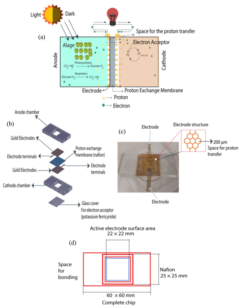
2. µPSC Operation and Fabrication

The principle of operation of the µPSC is the natural photosynthesis and respiration process. The µPSC involves the membrane electrode assembly sandwiched between the anode and cathode chambers. In the anode, photosynthesis drives the water-splitting reaction and releases electrons. In contrast, in the respiration process, electrons are also released by the catabolic activity of the photosynthetic microorganisms. These electrons traverse through electrodes in the membrane electrode assembly. Figure 1a demonstrates the principle of operation of the µPSC. As the detailed principle of operation is presented in our previous works, the authors recommend referring to [3,8,11].

Photosynthesis

$$6C{O}_2+6H_{2}O\stackrel{\hspace{1em}\downarrow \downarrow \downarrow \left(Light\right)\hspace{1em}}{\to }{C}_6{H}_{12}{O}_6+6O_2$$

(1)

Respiration

$$C_6{H}_{12}{O}_6+6O_2\stackrel{\hspace{1em}\hspace{1em}}{\to }6C{O}_2+6H_{2}O$$

(2)

3. µPSC Fabrication

The µPSC comprises two chambers: anode and cathode. Both chambers are separated by the proton exchange membrane (PEM). The microelectrodes were fabricated on both sides of the PEM. The microelectrodes comprised a thin aluminum honeycomb-structured arrayed grid coated with 40 nm gold through the sputtering technique. The electrode-patterned PEM was sandwiched between the anode and cathode chambers. The cathode chamber was sealed with a microscopic glass slide to hold the electron acceptor (potassium ferricyanide). Figure 1b illustrates the various components and assemblies of the µPSC. Figure 1c shows the photo image of the assembled µPSC. The detailed dimensions of the whole µPSC are shown in Figure 1d. As the focus of this work is on the modeling of the µPSC, for fabrication and experimental details, it is suggested to refer to our previous work [3,8,30]. The micro-photosynthetic power cells have been evaluated under an illumination level of 2 µmolm⁻²s⁻¹, which has consistently demonstrated superior performance compared to other lighting conditions. Consequently, all characterizations have been conducted under this specific illumination setting [29].

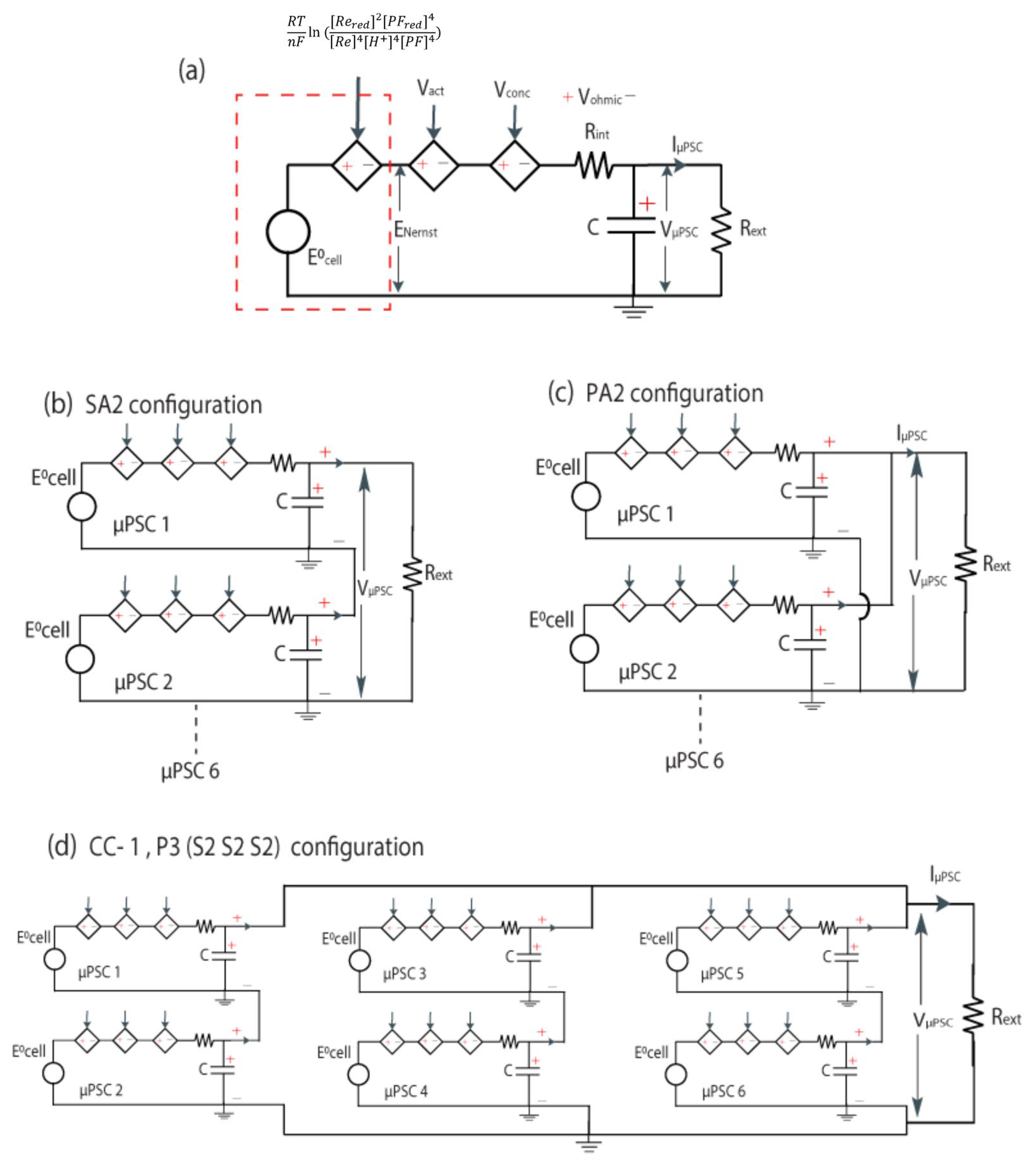
4. Modeling the Electrical Equivalent Circuit of a Single µ-PSC

The terminal voltage of the µPSC is the Nernst reversible voltage with µPSC internal losses such as activation voltage loss, concentration voltage loss, and ohmic voltage loss. Hence, the terminal voltage could be written as

$$V=E_0-V_{act}-V_{conc}-V_{ohmic}$$

(3)

where,

$V$—Voltage of the µPSC measured across terminals (V)

$E_0$—Nernst reversible voltage (V)

$V_{act}$, activation voltage loss = $\frac{RT}{\alpha F}{\sinh }^{-1}(\frac{i}{2{\mathit{i}}_0})$

$V_{conc}$, concentration voltage loss = $\left(\frac{-RT}{nF}\ln (1-\frac{i}{i_L})\right)$

$V_{ohmic}$, Ohmic voltage losses = $R_{ohmic}i$

The activation, concentration, and Ohmic losses were directly substituted from the work [29]. where,

R	Universal gas constant (8.31447 J/mol-K)
T	Operating temperature (Room temperature, (298.15 K)
F	Faraday’s constant (96,486 C/mol)
n	Number of transferred electrons/reactions (4 mol)
$i_L$	Limiting current density (0.1818 mA/cm2)
$i_0$	Equilibrium exchange current density (10−8 A/cm2)
$R_{ohmic}$	Ohmic resistance (Ω)

All these parameters are constants [29]. The Nernst Reversible voltage is given by,

$$E_0=E_{cell}^0-\frac{RT}{nF}ln\left(\frac{{[R{e}_{red}]}^2{[P{F}_{red}]}^4}{{\left[Re\right]}^4{[H^{+}]}^4{[PF]}^4}\right)$$

(4)

The anode chamber of the µPSC consist of anolyte (algal cells with electron mediators’ methylene blue). The cathode chamber consists of electron acceptors (potassium ferricyanide). The oxidation and reduction of methylene blue and electron acceptors potassium ferricyanide during the process are the reactants and products.

The electrical equivalent circuit of the single µPSC is shown in Figure 2a [29]. In the Nernst reversible voltage, $E_{cell}^0$ of the µPSC is modelled as DC voltage source and reactants and products were modelled as controlled voltage source, which is the function of the rate of change in the anode and cathode species concentration. The rate of change of species concentration is the solution of a set of first-order differential equations [28]. Both the activation and concentration voltage losses were modeled as controlled voltage sources. The Ohmic loss is represented as the resistive element. The proton exchange membrane is modeled as a capacitor. The resistive load is connected to the terminals of the µPSC [29]. Figure 2b shows the electrical equivalent model of the two µPSCs in series connection and Figure 2c shows the electrical equivalent model of the two µPSCs in parallel connection. Figure 2d shows the electrical equivalent circuit of a combination of series and parallel connections of the µPSC.

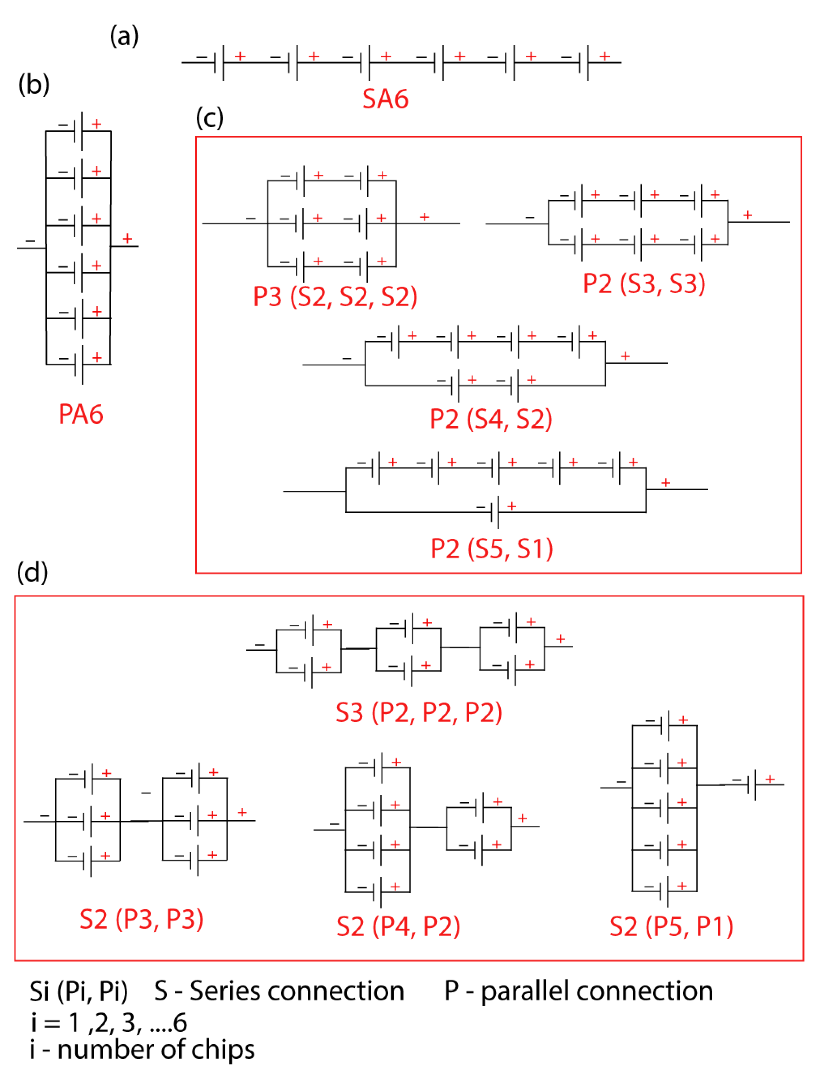
5. Modeling Array Configurations of µ-PSCs

5.1. SA6 Configuration

In the SA6 configuration, the µPSCs were connected in series connections. The six µPSCs were all connected in series (Figure 3a).

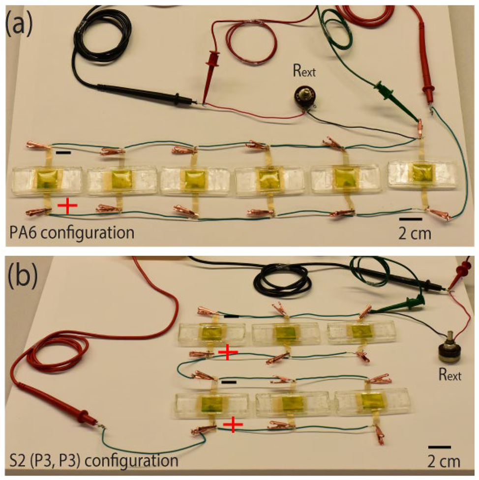
5.2. PA6 Configuration

In the PA6 configuration, the µPSCs were connected in parallel. The first µPSCs anode and sixth µPSCs cathode terminals were connected to the DAQ for the current and voltage sensing (Figure 3b). The photo image of the PA6 configurations is shown in Figure 4a.

5.3. Combinatory Configuration (CC-1)

To observe the performance of the µPSCs in sequences of series and parallel configurations, four unique configurations were chosen to analyze the performance. In the [P3 (S2, S2, S2)] configuration, two µPSCs were connected in series, and such three sets were connected in parallel connection (Figure 3c). In other configurations, two sets of three µPSCs were connected in series; then, both the sets were connected in parallel connection [P2 (S3, S3)]. In [ P2 (S4, S2)] configuration, four µPSCs were connected in series, and separate two µPSCs were connected in series then both sets were connected in parallel. In [P2 (S5, S1)] configuration, the five µPSCs were connected in series connection, and single µPSC were connected in parallel connection.

5.4. Combinatory Configuration (CC-2)

In the CC-2 configuration four unique configurations were chosen. In the [S3 (P2, P2, P2)] configuration, two µPSCs were connected in parallel, and three sets of such parallel connections were connected in series connection (Figure 3d). In configuration S2 (P3, P3), two sets of three µPSCs were connected in parallel, and then both the sets were connected in series connection. A photo image of this configuration is shown in Figure 4b. In S2 (P4, P2) configuration, four µPSCs were connected in parallel and two µPSCs were connected in parallel, then both sets were connected in series. In the last CC-2 configuration, five µPSCs were connected in parallel connection, and single µPSC were connected in a series connection to that [S2 (P5, P1)].

The experimental performances of the µPSCs may differ due to variations in the fabrication and also transient parameters such as rate of changes in species concentration, illumination on the surface of the anode chamber, and many more. Therefore, for simplicity and to demonstrate the capacity of the model for the arrayed configurations, normalized values are presented to analyze the I-V and I-P characteristics of the array of the µPSCs. The normalized voltage of the µPSC is calculated as, $Vr=\frac{V}{V_{oc}}$, where V is the terminal voltage of the µPSC and Voc is the open circuit voltage of the µPSC. The similarly normalized current of the µPSC is calculated as, $Ir=\frac{I}{I_{sc}}$, where I, is the µPSC current and Isc is the short circuit current of the µPSC. The normalized power of the µPSC is calculated as, $Pr=\frac{P}{P_{mp}}$, where P is the power of the µPSC and Pmp is the maximum power of the µPSC.

6. Results and Discussion

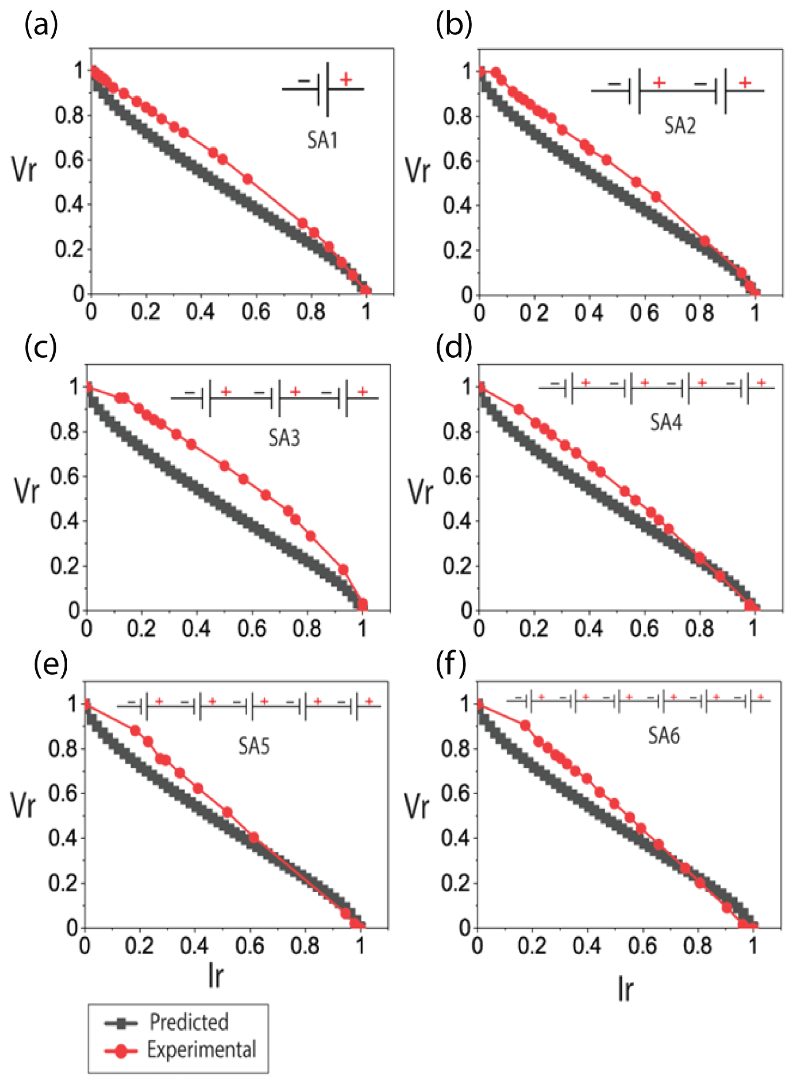
6.1. Polarization (I-V) Characteristics of SA6 Configuration

The I-V polarization characteristics are vital to comprehending the performance of the power-generating device. The I-V characteristics could be exploited to design suitable power converters for practical applications. Figure 5b demonstrates the normalized I-V characteristics of the SA2 configuration. In the SA2 configuration, the effective terminal voltage was the sum of their terminal voltages (

Table 1. Real-time predicted and experimental Voc, Isc, and Pmp of SA6 configurations.

Array	(Voc) mV		(Isc) µA		(Pmp) µW
	Predicted	Experimental	Predicted	Experimental	Predicted	Experimental
SA1	848.6	780	800	820	180	186
SA2	1697	1404	800	500	314	202
SA3	2545	2101	800	370	472	271
SA4	3394	3000	800	340	629	285
SA5	4243	3700	800	334	786	330
SA6	5091	4200	800	410	944	474

). In contrast, the effective current remained the same as that of the least µPSCs current in this array configuration.

In the model, all of the µPSCs utilized in array configurations demonstrated consistent performance because of consistent transient parameters. In contrast, the experimental results exhibited distinct performance, mainly because of the inconsistent performances of the µPSCs due to the uncontrolled transient parameters, which are yet to be understood in detail. Another significant reason for the inconsistent performance is the non-uniformity of the fabrication and transient behaviors [3,8].

Figure 5c reveals the SA3 configuration. In the model in the series configurations, the effective current remained unchanged at 800 µA, whereas the effective voltage was observed to be the summation of their voltages (Table 1). Figure 5d–f demonstrated the SA4, SA5, and SA6 configurations. Here, similar observations as those of the SA2 and SA3 configurations were also made. In the SA6 configuration, the effective voltage was the sum of their voltages, and the effective current remained the same as those of the least-performing µPSCs (Table 1).

6.2. Polarization (I-V) Characteristics of PA6 Configuration

Figure S1 demonstrates the normalized I-V characteristics of the PA6 configuration. In parallel configurations, the effective voltages remained identical to those of the least-performing µPSCs voltage (

Table 2. Real-time predicted and experimental Voc, Isc, and Pmp of PA6 configurations.

Array	(Voc) mV		(Isc) µA		(Pmp) µW
	Predicted	Experimental	Predicted	Experimental	Predicted	Experimental
PA1	848.6	780	800	820	180	186
PA2	848.6	725	1600	880	314	183.96
PA3	848.6	765	2400	1480	472	308.7
PA4	848.6	675	3200	1700	629	256
PA5	848.6	736	4000	2400	786	496.2
PA6	848.6	730	4800	2600	944	412.5

). In contrast, the effective current of the configuration was the sum of their µPSCs currents. For the PA2 configuration, experimental results demonstrated a current of 840 µA, whereas the predicted current demonstrated 1600 µA. The lower performance of the current in the experimental results was because of the meager performance of the µPSC owing to its inconsistent fabrications. The predicted current of 1600 µA indicated two µPSCs in parallel could potentially increase the mentioned performance using consistent fabrication of the µPSCs. Similar observations were made in the PA3, PA4, PA5, and PA6 configurations. Their effective terminal voltages almost remained the same as those of the least-performing µPSCs voltage. In contrast, their effective current was the sum of their µPSCs current (Table 2). In the PA6 configuration, a maximum effective voltage of 800 mV and a current of 4800 µA were predicted.

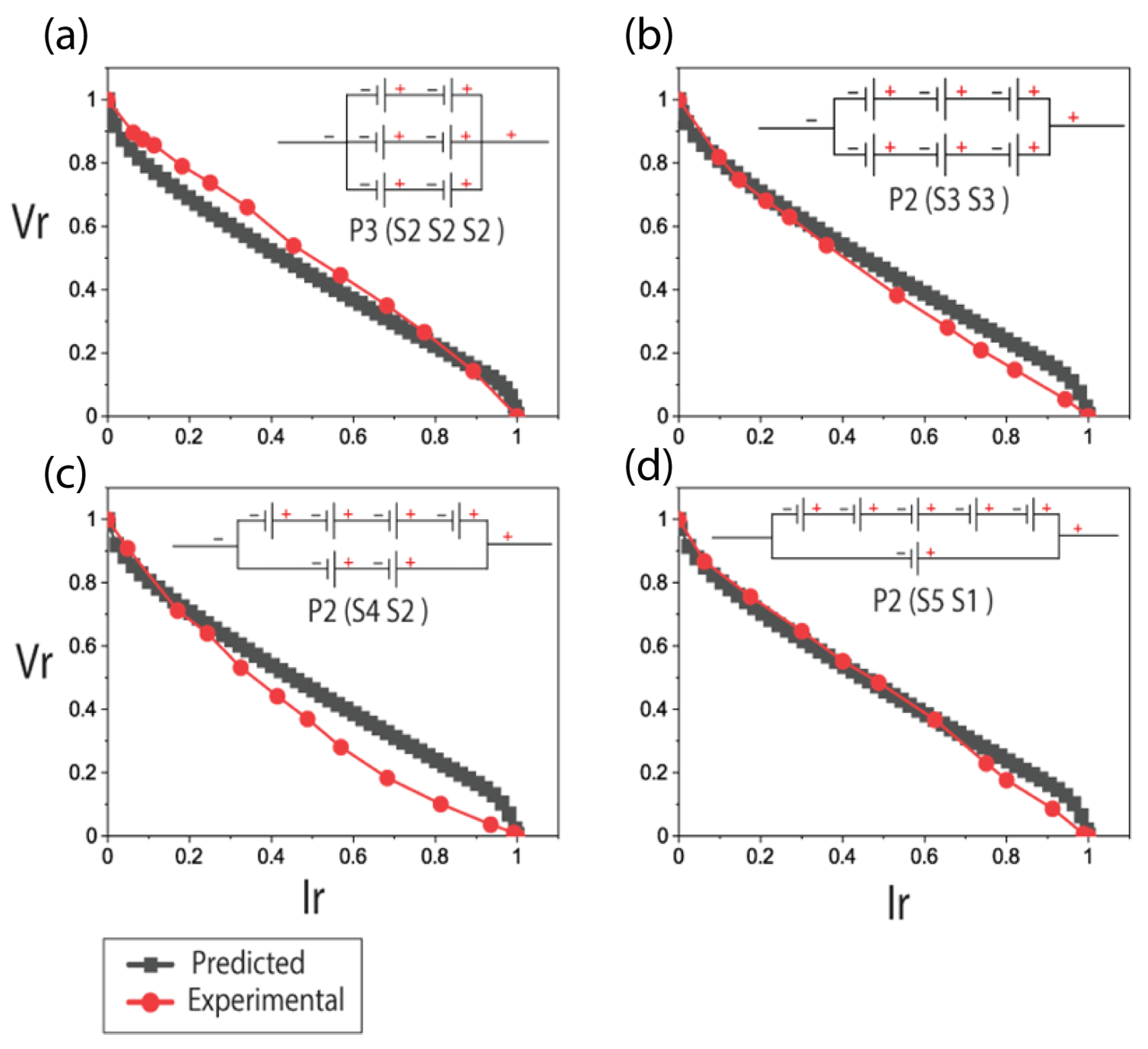
6.3. Polarization (I-V) Characteristics of CC-1 Configuration

The effective terminal voltages of the µPSCs were increased in the series configurations, and effective µPSCs currents remained the least µPSCs current. In contrast, the effective µPSC currents were enhanced in the parallel configurations, and their effective voltage remained the least-performing µPSC. Based on this understanding, to enhance both the effective voltage and effective µPSCs current of the arrayed µPSCs different array combinations of series and parallel were chosen.

Figure 6a demonstrates the normalized I-V characteristics of the [P2 (S2, S2, S2)] combination of the CC-1 configuration. The predicted values were slightly greater than the experimental values, indicating that the experimental µPSC current could be boosted by consistent fabrication (

Table 3. Real-time predicted and experimental Voc, Isc, and Pmp of CC-1 configurations.

CC-1	(Voc) mV		(Isc) µA		(Pmp) µW
	P	E	P	E	P	E
P3 (S2,S2,S2)	1839	1550	2400	1760	985	616
P2 (S3,S3)	2741	2430	1600	1220	1026	624
P2 (S4,S2)	2438	2800	1600	1230	912	396
P2 (S5,S1)	1526	1302	1600	800	570	246

). In this combination, both effective voltages and currents were enhanced. Figure 6b reveals the normalized I-V characteristics of the [P2(S3, S3)] combination. Herein, the experimental results were almost matching the predicted values, whereas the experimental currents were slightly less than the predicted values. However, it was found that in both of these combinations, voltages and currents were enhanced.

Figure 6c shows the normalized I-V characteristics of the [P2 (S4, S2)] configuration. The predicted effective terminal voltages were slightly lower than the experimental value, perhaps because of the increase in the voltage in the long-term performance (Table 3) [10]. Figure 6d shows the normalized I-V characteristics of the [P2 (S5, S1)] configuration. The effective terminal voltages of the experiment were almost close to the predicted values. However, the effective currents of the experiment were quite lower than the predicted ones.

6.4. Polarization (I-V) Characteristics of CC-2 Configuration

To observe the performance of the µPSCs in combinations of parallel configurations, unique parallel combination strategies were chosen. Their corresponding normalized I-V characteristics were simulated and validated with the experimental results. Figure S2a demonstrates the normalized I-V characteristics of the CC-2 configuration [S2 (P2, P2, P2)]. Figure S2b demonstrates the [S2 (P3, P3)] configuration. Here, it was observed that experimental terminal currents were slightly higher than the predicted currents, perhaps because of a higher rate of electron transfer to the electrode surface, which is not considered in the modeling (

Table 4. Real time predicted and experimental Voc, Isc, and P_mp of CC-2 configurations.

CC-2	(Voc)		(Isc)		(Pmp)
	P	E	P	E	P	E
S3 (P2, P2, P2)	2741	2300	1600	1390	1026	869
S2 (P3, P3)	1839	1475	2400	2100	985	926
S2 (P4, P2)	1833	1680	1600	1820	887	777
S2 (P5, P1)	1826	1530	800	960	561	141

). Figure S2c shows the [S2 (P4, P2)] configuration. Here too, similar observation was made, like that of the [S2 (P3, P3)] configuration. Figure S2d shows the normalized I-V characteristics of the [S2 (P5, P1)].

6.5. I-P Characteristics

The current—Power (I-P) characteristics provide the maximum power of the typical power generating device—these aid to design the appropriate power converters for maximum power enhancement. Figure 7 demonstrates the normalized I-P characteristics of the µPSC array configurations.

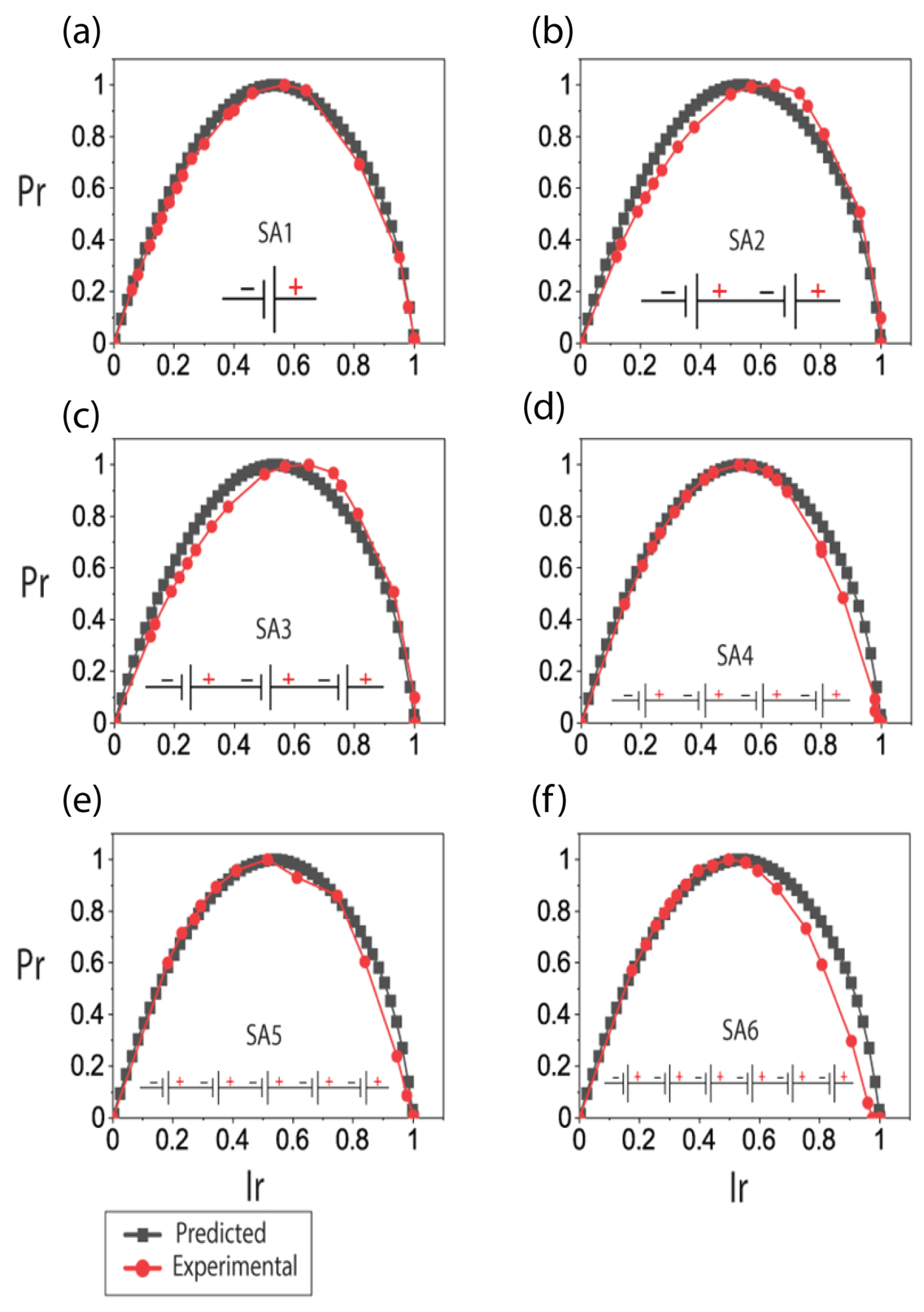
6.6. I-P Characteristics of SA6 Configuration

Figure 7b demonstrates the normalized I-P characteristic of the SA2 configuration. The predicted values indicate that the experimental power could be enhanced up to the maximum potential predicted by the modeling for the said dimensions (Table 1). Similar observations were made with the SA3, SA4, SA5, and SA6 configurations. From the simulation, it was realized that by adding a greater number of µPSCs in series, its power output could be enhanced. The enhancement factor follows the linear relationship, provided all the µPSCs in that configuration have the same performance (Table 1). One of the µPSC’s lower performances leads to lower effective performance. In all the SA6 configurations, the current has remained the same, and the voltage increased with an increase in the number of µPSCs. The increase in the voltage has led to increased power output in the SA6 configuration.

6.7. I-P Characteristics of PA6 Configuration

Figure S3b demonstrates the normalized I-P characteristic PA2 configuration. The predicted maximum power indicated that in the parallel connection, both current and power could be enhanced by increasing the number of µPSCs. The similar observations were made in PA3 (Figure S3c), PA4 (Figure S3d), PA5 (Figure S3e) and PA6 (Figure S3f) configuration.

6.8. I-P Characteristics of CC-1 Configuration

Figure S5a demonstrates the normalized I-P characteristics of the [P2 (S2, S2, S2)] configuration. Compared to the SA6 and PA6 configurations, the combination of series and parallel µPSCs has demonstrated higher maximum power. In this array configuration, the model has predicted a maximum power (Pmp) of 1000 µW, indicating the maximum power that could be potentially generated by this array configuration. Similar observations were made with [P2 (S3, S3)] (Figure S5b), [P2 (S4, S2)] (Figure S5c) and P2 (S5, S1) (Figure S5d) configurations.

6.9. I-P Characteristics of CC-2 Configuration

Figure S4a demonstrates the normalized I-P characteristics of the CC-2 configuration’s [S2 (P2, P2, P2)] configuration. Compared to all other configurations, the [S2 (P2, P2, P2)] configuration has generated higher maximum power than any other combination. In the case of combination [S2 (P4, P2)] and [S2 (P5, P1)], the experimental currents were slightly greater than the predicted values, perhaps because of the higher rate of electron transport in the long-term performance of the µPSCs, which was not considered in the modeling (Table 4).

The combinations [S2 (P4, P2)] (Figure S4c) and [S2 (P5, P1)] (Figure S4d) have shown a slightly different pattern than the other combinations. Both experimental and predicted I-P characteristics showed slightly different patterns, which perhaps indicates slightly different phenomena with these combinations. More investigations are necessary to understand the underlying phenomenon of this combination. Moreover, both combinations’ effective terminal voltage and currents were much lower than all other combinations in this study.

6.10. Variation of Open-Circuit Voltage (Voc), Short Circuit Current (Isc), Load Voltage (V_L), and Load Current (I_L)

6.10.1. Variation of Open-Circuit Voltage (Voc)

In the case of the SA6 configuration, the model has predicted slightly higher values than the experimental values, indicating the experimental values could be potentially enhanced by the consistent performances of all the µPSCs in an array configuration. In the SA2 configuration, experimental values have demonstrated a slightly lower Voc of 1404 mV compared to the predicted value of 1697 mV. In the SA3 configuration, experimental values have demonstrated a Voc of 2101 mV, while the model has predicted 2550 mV. It was observed that with an increase in the number of µPSCs in series connection, the losses (ohmic) in the circuit have increased. This indicates that the Voc of the effective array of µPSCs in series connections is the summation of the individual Voc with ohmic losses in the circuit.

In the PA6 configuration, the effective Voc was the result of the least-performing µPSC’s Voc. Here, the predicted values remained at 848. A total of 8 mV, while the experimental values varied in the range of 675 mV to 765 mV. However, the variation is insignificant.

The experimental values of [P2 (S2,S2,S2)], [P2 (S3,S3)], and [P2 (S5,S1)] were slightly less than the predicted values. In these combinations, the difference between experimental and predicted values was insignificant. The combination [P2 (S4, S2)] has predicted a slightly lower Voc than the experimental value, perhaps because, in the long run, the Voc has increased during the experimental section.

The combination [S2 (P2, P2, P2)] has demonstrated a higher Voc than the experimental value, indicating the possibility of improving the performance of the µPSC with consistent performance. In all other combinations, the experimental values were slightly less than the predicted values.

6.10.2. Variation of Short Circuit Current (Isc)

In the SA6 configuration, the effective Isc has remained the least-performing µPSC Isc. The predicted Isc has remained at 800 µA in all series configurations of µPSCs. Theoretically, the experimental values should be closer to the predicted values; however, due to the inconsistent performance of the µPSCs, the experimental results demonstrated slightly lesser values (Table 1).

In a parallel connection, effective Isc was the summation of the individual Isc of the µPSCs. The two µPSCs in parallel connection have a predicted Isc of 1600 µA. It was observed that as the number of µPSCs increased in the parallel connection, the Isc increased. It was the linear summation of the individual µPSCs Isc (Table 2).

The combination [P2 (S2, S2, S2)] has demonstrated a difference of 480 µA from their predicted values. The combination [P2 (S3, S3)] has demonstrated a 300 µA lesser value than their predicted values. Similar observations were made with [P2 (S4, S2)]. Only the combination [P2 (S5, S1)] has shown a higher difference of 800 µA compared to their predicted values. It was observed that these combinations generated near values similar to those of their corresponding predicted values.

The [S2 (P2, P2, P2)] has shown a slight difference of 220 µA compared to their predicted value of 1600 µA. The combination [S2 (P3, P3)] has demonstrated a difference of 200 µA from their predicted values. The combination [P2 (S4, S2)] has a slightly higher experimental Isc than the predicted values. The combination [P2 (S5, S1)] has also shown a slightly higher experimental value than predicted values. The main reason might be µPSCs dynamics. During the dynamics, their performance may have increased, as in the long run, the µPSCs performance increases. Furthermore, these operation dynamics were not considered in the modeling.

6.10.3. Variation of Load Voltage (V_L) and Current (I_L) at 1 kΩ

To observe the performance of µPSC under real-time loading conditions, a load test at 1 kΩ was simulated for all array configurations. The resistance of 1 kΩ was connected to the terminals of the µPSC, and their corresponding terminal voltage and currents were recorded. Further, their predicted results were compared with experimental results.

The µPSC follows the ohms law. When the load resistance was set to 1 kΩ, their voltages and currents were the same. Therefore, separate load currents were not provided. The V_L and I_L were provided in mV and µA, respectively.

Figure S6a illustrates the V_L of the SA6 configuration. For all six µPSCs in series connection, the model has predicted a V_L of 661 mV. However, the experimental values varied in the range of 322 to 370 mV due to variations in their performances. The number of µPSCs increased, but their V_L was not increased, indicating that for real-time loading conditions, these connections are ineffective. Similar observations were made with load currents as well, and currents are in µA.

Figure S6b shows the V_L of the PA6 configuration. The parallel-connected µPSCs have demonstrated a higher V_L than the series-connected µPSCs. The two µPSCs in parallel configurations have demonstrated a V_L of 450 mV, whereas the model has predicted 559 mV. In this configuration, an increase in the V_L was observed with an increase in the number of µPSCs in parallel connection. For PA3 configuration, the model has predicted a V_L of 605 mV, and with PA6 configuration, the model has predicted a V_L of 660 mV. With an increase in the number of µPSCs in parallel connection, V_L was found to be increased. A similar trend was observed with experimental results too. As the number of µPSCs increased in the parallel configurations, their corresponding V_L increased. Though there are some discrepancies in the values, the overall trend increased with an increase in the number of µPSCs in parallel connection, and therefore, compared to the series connection of µPSCs, parallel configurations have a slightly increasing trend with an increase in the number of µPSCs.

Figure S6c illustrates the V_L of CC-1 configurations. For the combination [P2 (S2, S2, S2)], the model has predicted a higher V_L than the series (SA6) and parallel (PA6) configurations. This combination has predicted a V_L of 1039 mV, whereas the experimental values demonstrated a value of 800 mV. The difference of 239 mV is perhaps because of the ohmic losses and inconsistent performances of the µPSCs in the array configurations. For the combination [P2 (S3, S3)], the model has predicted a V_L of 909 mV, whereas the experimental value has demonstrated a value of 800 mV. The combination of [P2 (S4, S2)] and [P2 (S5, S1)] experimental and predicted values is shown in Figure S6c. In all the combinations, it was observed that the predicted V_L was much higher than the experimental values of series and parallel configurations.

Figure S6d shows the CC-2 configuration µPSCs. Here it was found that the experimental V_L was much higher than the predicted values, perhaps because µPSC has shown an increasing trend with long-term operation. The long-term performance dynamics are not included in the modeling.

Among all these four different array configurations, it was found that the CC-1 and CC-2 configurations have demonstrated higher V_L and I_L than the only series and parallel connected µPSCs. Therefore, for real-time loading conditions, the combinations of series and parallel connections were considered the optimal strategies.

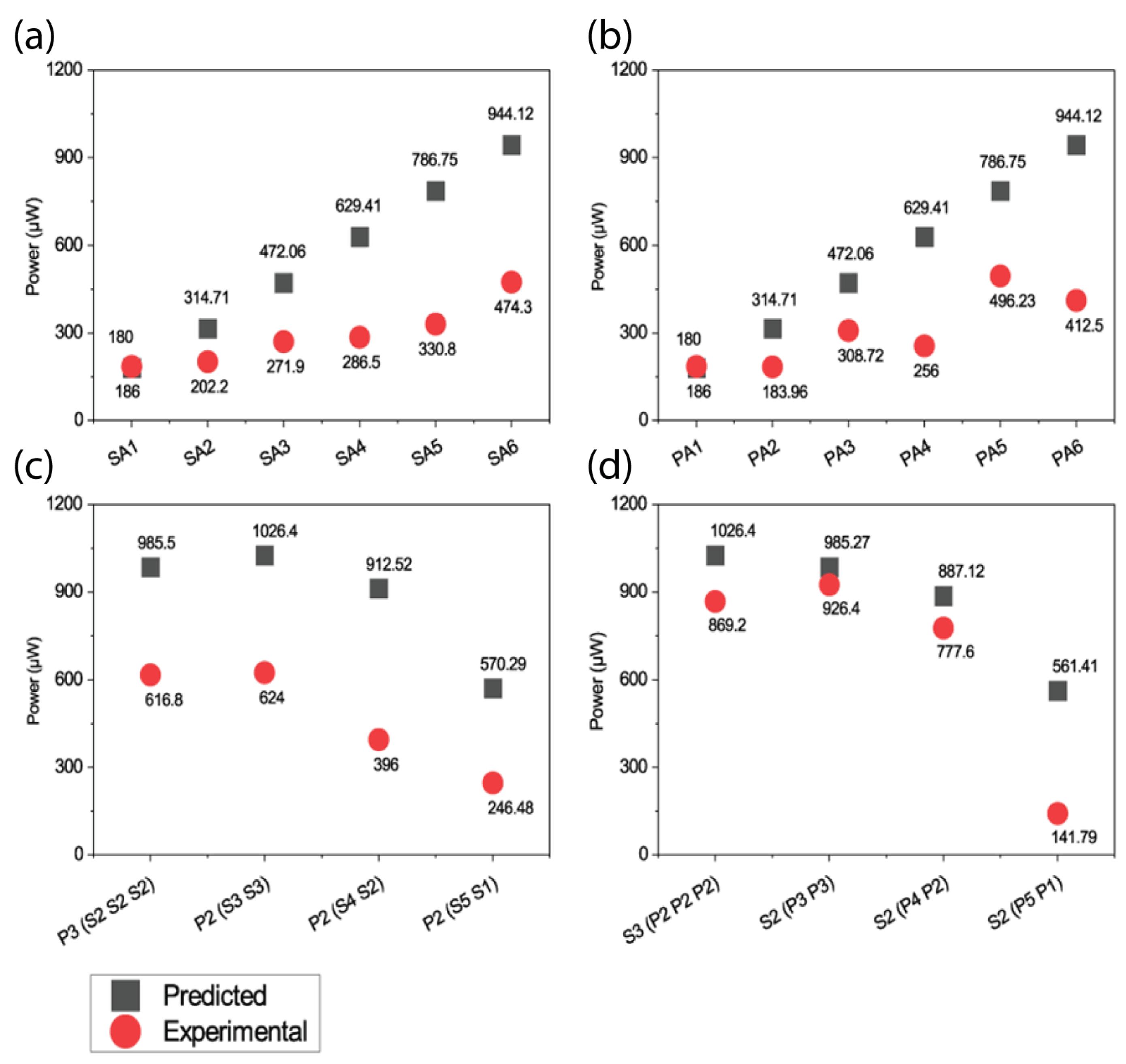
6.10.4. Variation of Maximum Power (P_mp) of Array Configurations

P_mp is the highest power generated from the µPSCs. Figure 8a demonstrates the P_mp of an array of µPSCs in the SA6 configuration. According to the model, it was observed that the maximum power increased with an increase in the number of µPSCs in the series connection. For the SA2 configuration, the model has predicted a P_mp of 359.9 µW, whereas the experimental value has shown 202.2 µW (Table 1). The lower experimental value was mostly perhaps because of the inconsistent performances of the µPSCs and ohmic losses in the circuit. The six µPSCs in series connection have a predicted P_mp of 1079.9 µW. Overall, in the series connection of µPSC, the P_mp has observed an increasing trend.

Figure 8b shows the P_mp of the PA6 configuration. Also, with an increase in the number of µPSCs, an increase in the P_mp was observed. For six µPSCs in parallel connection, the model has predicted a P_mp of 908.2 µW. Overall, an increase in the number of µPSCs in parallel connections was observed. However, series-connected µPSCs have demonstrated a slightly higher P_mp compared to parallel-connected µPSCs.

Figure 8c shows the P_mp of CC-1 configurations. For the combination [P2 (S2, S2, S2)], the model has predicted a P_mp of 985.5 µW, whereas the experimental values have demonstrated 616.8 µW. The combination [P2(S3, S3)] has predicted a P_mp of 1026.4 µW, and whereas the experiment has demonstrated 624 µW. The combination [P2(S4, S2)] and [P2 (S5, S1)] has predicted a slightly lower P_mp than the experimental values.

Figure 8d shows the Pmp of the CC-2 configuration. The combination [S2 (P2, P2, P2)] has predicted a Pmp of 1026.4 µW, whereas the experimental results have demonstrated a closer value of 869.2 µW. The combination [S2 (P3, P3)] model has predicted 985.27 µW. In contrast, the experimental values have predicted s value of 926.4 µW, which is close to the predicted one. For the combinations [S2 (P4, P2)] and [S2 (P5, P1)], the model has predicted values lower than the other two combinations.

In the comparison of P_mp, V_L, and I_L currents at 1 kΩ amongst all the array configurations, it was found that CC-1 and CC-2 configurations that too combinations [P2 (S2, S2, S2)], [P2 (S3, S3)] and [S2 (P2, P2, P2)], [S2 (P3, P3)] have demonstrated higher performance both experimentally and with predicted ones. From the model, it is understood that these configurations could be utilized for real-time applications where one can increase both voltages and currents.

6.11. Fill Factor (FF)

Fill factor is the ratio of maximum power obtained by the µPSC to the product of open circuit voltage and short circuit current of the µPSC.

$$Fill factor \left(FF\right)=\frac{P_{mp}}{\left(V_{oc}\times I_{sc}\right)}$$

(5)

Figure S7 shows the I-V and I-P characteristics demonstrating the fill factor. The FF of all the predicted array configurations is calculated and presented in

Table 5. Fill factor of all array configurations.

Array	FF	Array	FF
SA1	0.267	PA1	0.267
SA2	0.245	PA2	0.233
SA3	0.236	PA3	0.234
SA4	0.238	PA4	0.234
SA5	0.233	PA5	0.233
SA6	0.236	PA6	0.234
S3 (P2, P2, P2)	0.237	P3 (S2, S2, S2)	0.228
S2 (P3, P3)	0.228	P2 (S3, S3)	0.237
S2 (P4, P2)	0.307	P2 (S4, S2)	0.237
S2 (P5, P1)	0.389	P2 (S5, S1)	0.237

.

Table 5 shows the FF of the SA6 configurations. It was observed that the FF of the SA6 configurations varied from 0.233 to 0.267. For the single µPSC, FF was found to be 0.267. In contrast, the FF for the SA2 configurations was observed as 0.245. For SA3, SA4, SA5, and SA6 configurations FF variations are insignificant. Similar observations were made with PA6 and CC-1 configurations too. Here also the variation is insignificant. However, in CC-2, S2 (P4, P2) configuration FF was found to be 0.307. In S2 (P5, P1), configuration FF was found to be 0.389. Amongst all of the array configurations, the CC-1 P3 (S2, S2, S2) configuration and the CC-2 S2 (P3, P3) configuration have shown the lowest FF of 0.228. A maximum power of 985 µW was predicted with these configurations. In addition, the conversion efficiency of the micro-photosynthetic power cell, which is discussed in this manuscript, has a light input to electricity conversion efficiency of 0.18%. This is smaller in comparison with conventional photovoltaic cells. However, the micro-photosynthetic power cell is in its infancy stage. With advancements in technology, conversion efficiency will improve. Detailed research on the conversion efficiency of light energy to electricity is published in our previous works [15]. Moreover, comparing conventional photovoltaic (PV) solar cells, typically silicon-based, with bio-solar cells involves evaluating their energy conversion efficiencies and operation lifetimes. Conventional silicon-based PV cells exhibit higher efficiencies, ranging from 15% to 22%, with monocrystalline panels being the most efficient (around 20–22%). These cells are renowned for their long-term stability, often maintaining efficiency for over 25 years. In contrast, bio-solar cells, employing biological materials like algae or bacteria, generally achieve lower efficiencies (0.1% to 8%) and face challenges due to the limitations of biological organisms and sensitivity to environmental factors. Operational lifetimes for bio-solar cells are still a subject of research and development, while silicon-based PV panels are known for their durability and established warranties of 25 years or more.

7. Conclusions

This study presents a comprehensive investigation into the performance of array configurations of micro-photosynthetic power cells (µPSCs). Through rigorous modeling and experimental validation, we explored various array configurations, including series, parallel, and combinations thereof, under real-time loading conditions. Our findings reveal that combinations of series and parallel arrays of µPSCs are more effective in generating optimal power compared to configurations that utilize solely series or parallel connections. This insight is crucial for the practical application of µPSCs in powering low- and ultra-low-power devices. The study’s primary contribution lies in the proposed model’s versatility and applicability across various array configurations, enabling a deeper understanding of the performance characteristics of µPSC arrays. The polarization characteristics, current-voltage (I-V), and current-power (I-P) profiles of these arrays were validated against experimental results, affirming the model’s robustness. Furthermore, the study’s findings indicate that the devised array configurations, particularly those combining series and parallel arrangements, are promising for real-time applications where a balance of voltage and current is essential. This research not only advances the understanding of µPSCs in array configurations but also paves the way for future studies focusing on optimizing these systems for practical energy harvesting applications. The integration of µPSCs into the realm of sustainable energy sources represents a significant stride forward, potentially impacting various sectors reliant on low-power solutions. Further research is required to enhance the efficiency and stability of these bio-inspired energy systems, ensuring their viability in real-world applications.

References

1. Dresselhaus, M.S.; Thomas, I.L. Alternative energy technologies. Nature 2001, 414, 332–337. [Google Scholar] [CrossRef] [PubMed]
2. Kuruvinashetti, K.; Guoqing, G.; Haobin, J.; Packirisamy, M. Perspective—Application of Micro Photosynthetic Power Cells for IoT in Automotive Industry. J. Electrochem. Soc. 2020, 167, 037545. [Google Scholar] [CrossRef]
3. Tanneru, H.K.; Kuruvinashetti, K.; Pillay, P.; Rengaswamy, R.; Packirisamy, M. Perspective—Micro photosynthetic power cells. J. Electrochem. Soc. 2019, 166, B3012. [Google Scholar] [CrossRef]
4. Saar, K.L.; Bombelli, P.; Lea-Smith, D.J.; Call, T.; Aro, E.M.; Müller, T.; Howe, C.J.; Knowles, T.P. Enhancing power density of biophotovoltaics by decoupling storage and power delivery. Nat. Energy 2018, 3, 75–81. [Google Scholar] [CrossRef]
5. Sawa, M.; Fantuzzi, A.; Bombelli, P.; Howe, C.J.; Hellgardt, K.; Nixon, P.J. Electricity generation from digitally printed cyanobacteria. Nat. Commun. 2017, 8, 1327. [Google Scholar] [CrossRef]
6. Bombelli, P.; Müller, T.; Herling, T.W.; Howe, C.J.; Knowles, T.P.J. A High Power-Density, Mediator-Free, Microfluidic Biophotovoltaic Device for Cyanobacterial Cells. Adv. Energy Mater. 2015, 5, 1401299. [Google Scholar] [CrossRef]
7. McCormick, A.J.; Bombelli, P.; Bradley, R.W.; Thorne, R.; Wenzel, T.; Howe, C.J. Biophotovoltaics: Oxygenic photosynthetic organisms in the world of bioelectrochemical systems. Energy Environ. Sci. 2015, 8, 1092–1109. [Google Scholar] [CrossRef]
8. Ramanan, A.V.; Pakirisamy, M.; Williamson, S.S. Advanced Fabrication, Modeling, and Testing of a Microphotosynthetic Electrochemical Cell for Energy Harvesting Applications. IEEE Trans. Power Electron. 2015, 30, 1275–1285. [Google Scholar] [CrossRef]
9. Ravi, S.K.; Yu, Z.; Swainsbury, D.J.; Ouyang, J.; Jones, M.R.; Tan, S.C. Enhanced output from biohybrid photoelectrochemical transparent tandem cells integrating photosynthetic proteins genetically modified for expanded solar energy harvesting. Adv. Energy Mater. 2017, 7, 1601821. [Google Scholar] [CrossRef]
10. Driver, A.; Bombelli, P. Biophotovoltaics. Catalyst. 2011, 13–15. [Google Scholar]
11. Bradley, R.W.; Bombelli, P.; Rowden, S.J.; Howe, C.J. Biological photovoltaics: Intra-and extra-cellular electron transport by cyanobacteria. Biochem. Soc. Trans. 2012, 40, 1302–1307. [Google Scholar] [CrossRef] [PubMed]
12. Yang, Y.; Gobeze, H.B.; D’Souza, F.; Jankowiak, R.; Li, J. Plasmonic enhancement of biosolar cells employing light harvesting complex II incorporated with core–shell metal@ TiO2 nanoparticles. Adv. Mater. Interfaces 2016, 3, 1600371. [Google Scholar] [CrossRef]
13. Robinson, M.T.; Armbruster, M.E.; Gargye, A.; Cliffel, D.E.; Jennings, G.K. Photosystem I multilayer films for photovoltage enhancement in natural dye-sensitized solar cells. ACS Appl. Energy Mater. 2018, 1, 301–305. [Google Scholar]
14. Wey, L.T.; Bombelli, P.; Chen, X.; Lawrence, J.M.; Rabideau, C.M.; Rowden, S.J.; Zhang, J.Z.; Howe, C.J. The development of biophotovoltaic systems for power generation and biological analysis. ChemElectroChem 2019, 6, 5375–5386. [Google Scholar] [CrossRef] [PubMed]
15. Kuruvinashetti, K.; Pakkiriswami, S.; Packirisamy, M. Gold Nanoparticle interaction in algae enhancing quantum efficiency and power generation in microphotosynthetic power cells. Adv. Energy Sustain. Res. 2022, 3, 2100135. [Google Scholar] [CrossRef]
16. Lam, K.B.; Irwin, E.F.; Healy, K.E.; Lin, L. Bioelectrocatalytic self-assembled thylakoids for micro-power and sensing applications. Sens. Actuators B Chem. 2006, 117, 480–487. [Google Scholar] [CrossRef]
17. Firoozabadi, H.; Mardanpour, M.M.; Motamedian, E. A system-oriented strategy to enhance electron production of Synechocystis sp. PCC6803 in bio-photovoltaic devices: Experimental and modeling insights. Sci. Rep. 2021, 11, 12294. [Google Scholar] [CrossRef]
18. Ng, F.-L.; Phang, S.-M.; Periasamy, V.; Beardall, J.; Yunus, K.; Fisher, A.C. Algal biophotovoltaic (BPV) device for generation of bioelectricity using Synechococcus elongatus (Cyanophyta). J. Appl. Phycol. 2018, 30, 2981–2988. [Google Scholar] [CrossRef]
19. Kim, M.J.; Bai, S.J.; Youn, J.R.; Song, Y.S. Anomalous power enhancement of biophotovoltaic cell. J. Power Sources 2019, 412, 301–310. [Google Scholar] [CrossRef]
20. Park, S.H.; Song, Y.S. Carbon nanofluid flow based biophotovoltaic cell. Nano Energy 2021, 81, 105624. [Google Scholar] [CrossRef]
21. Carbas, B.B.; Güler, M.; Yücel, K.; Yildiz, H.B. Construction of novel cyanobacteria-based biological photovoltaic solar cells: Hydrogen and photocurrent generated via both photosynthesis and respiratory system. J. Photochem. Photobiol. Chem. 2023, 442, 114764. [Google Scholar] [CrossRef]
22. Choi, D. Developing Sustainable Water and Electricity for Impoverished Regions using Algae-based Bio-Photovoltaics. Available online: https://www.gcrsef.org/wp-content/uploads/formidable/13/State-Research-Paper_Dorothy-Choi.pdf (accessed on 2 October 2023).
23. Chin, J.-C.; Khor, W.-H.; Chong, W.W.F.; Wu, Y.-T.; Kang, H.-S. Effects of anode materials in electricity generation of microalgal-biophotovoltaic system—Part I: Natural biofilm from floating microalgal aggregation. Mater. Today Proc. 2022, 65, 2970–2978. [Google Scholar] [CrossRef]
24. Amjadian, S.; Esmaeilzadeh, M.; Ajeian, R.; Riazi, G.; Ramakrishna, S. Efficiency Enhancement of Biophotovoltaic Solid-State Solar Cells. Energy Technol. 2023, 11, 2300337. [Google Scholar] [CrossRef]
25. Lee, S.J.; Song, J.J.; Lee, H.J.; Jeong, H.Y.; Song, Y.S. Enhanced energy harvesting in a bio-photovoltaic cell by integrating silver nanoparticles. J. Korean Phys. Soc. 2022, 80, 420–426. [Google Scholar] [CrossRef]
26. Liu, L.; Choi, S. Self-sustainable, high-power-density bio-solar cells for lab-on-a-chip applications. Lab. Chip 2017, 17, 3817–3825. [Google Scholar] [CrossRef] [PubMed]
27. Indro, M.N.; Maddu, A.; Eviana, E. Utilization of cyanobacteria in photovoltaic technology. IOP Conf. Ser. Earth Environ. Sci. 2019, 299, 012064. [Google Scholar] [CrossRef]
28. Tanneru, H.K.; Suresh, R.; Rengaswamy, R. On modeling and optimization of micro-photosynthetic power cells. Comput. Chem. Eng. 2017, 107, 284–293. [Google Scholar] [CrossRef]
29. Masadeh, M.A.; Kuruvinashetti, K.; Shahparnia, M.; Pillay, P.; Packirisamy, M. Electrochemical Modeling and Equivalent Circuit Representation of a Microphotosynthetic Power Cell. IEEE Trans. Ind. Electron. 2017, 64, 1561–1571. [Google Scholar] [CrossRef]
30. Kuruvinashetti, K.; Tanneru, H.K.; Pillay, P.; Packirisamy, M. Review on Microphotosynthetic Power Cells—A Low-Power Energy-Harvesting Bioelectrochemical Cell: From Fundamentals to Applications. Energy Technol. 2021, 9, 2001002. [Google Scholar] [CrossRef]
Figure 1. (a) Operating principle, (b) components of the µPSC, (c) photo image of the fabricated µPSC, (d) dimensions of the µPSC.
Energies 17 01749 g001
Figure 2. (a) Electrical equivalent circuit of the single µPSC, (b) equivalent circuit of two µPSCs in series connection, (c) equivalent circuit of two µPSCs in parallel connection, (d) equivalent circuit of P3 (S2, S2, S2) configuration.
Energies 17 01749 g002
Figure 3. (a) SA6 configuration of µPSCs (b) PA6 configuration of µPSCs (c) Combinatory configuration—1 (CC-1) of µPSCs, four combinations ([P3 (S2, S2, S2)], [P2 (S3, S3)], [P2 (S4, S2)], [P2 (S5, S1)]) (d) combinatory configuration—2 of µPSCs, four combinations ([S3 (P2, P2, P2)], [S2 (P3, P3)], [S2 (P4, P2)], [S2 (P5, P1)]).
Energies 17 01749 g003
Figure 4. Photo image of the array configurations of the µPSCs. (a) PA6 configuration (b) S2 (P3,P3) configuration.
Energies 17 01749 g004
Figure 5. Normalized I-V characteristics of SA6 configuration, (a) SA1 configuration, (b) SA2 configuration, (c) SA3 configuration, (d) SA4 configuration, (e) SA5 configuration, (f) SA6 configuration. Red circle lines represent the experimental results; black squares represent the simulated (predicted values).
Energies 17 01749 g005
Figure 6. Normalized I-V characteristics of CC-1 configuration. (a) [P2(S2, S2, S2)] configuration (b) [P2(S3, S3)] configuration (c) [P2(S4, S2)] configuration (d) [P2 (S5, S1)] configuration. The red circles represent the experimental results; black squares represent the simulated (predicted values).
Energies 17 01749 g006
Figure 7. Normalized I-P characteristic curves SA6 configuration. (a) SA1 configuration, (b) SA2 configuration, (c) SA3 configuration, (d) SA4 configuration, (e) SA5 configuration, (f) SA6 configuration. The circles represent the experimental results; black squares represent the simulated (predicted values).
Energies 17 01749 g007
Figure 8. Variation of Pmp of predicted and experimental results of all four array configurations. (a) SA6 configuration, (b) PA6 configuration, (c) CC-1 configuration, (d) CC-2 configuration.
Energies 17 01749 g008