
Transmission Expansion Planning Considering Storage, Flexible AC Transmission System, Losses, and Contingencies to Integrate Wind Power


Department of Electrical Engineering, Federal University of Rio de Janeiro, COPPE, Rio de Janeiro 21941-901, Brazil
*
Author to whom correspondence should be addressed.
Energies 2024, 17(7), 1777; https://doi.org/10.3390/en17071777
Submission received: 21 March 2024
/
Revised: 30 March 2024
/
Accepted: 6 April 2024
/
Published: 8 April 2024
(This article belongs to the Section F1: Electrical Power System)
Abstract
:To meet future load projection with the integration of renewable sources, the transmission system must be planned optimally. Thus, this paper introduces a comparative analysis and comprehensive methodology for transmission expansion planning (TEP), incorporating the combined effects of wind power, losses, N-1 contingency, a FACTS, and storage in a flexible environment. Specifically, the optimal placement of the FACTS, known as series capacitive compensation (SCC) devices, is used. The intraday constraints associated with wind power and energy storage are represented by the methodology of typical days jointly with the load scenarios light, heavy, and medium. The TEP problem is formulated as a mixed-integer nonlinear programming (MINLP) problem through a DC model and is solved using a specialized genetic algorithm. This algorithm is also used to determine the optimal placement of SCC devices and storage systems in expansion planning. The proposed methodology is then used to perform a comparison of the effect of the different technologies on the robustness and cost of the final solution of the TEP problem. Three test systems were used to perform the comparative analyses, namely the Garver system, the IEEE-24 system, and a real-world Colombian power system of 93 buses. The results indicate that energy storage and SCC devices lead to a decrease in transmission requirements and overall investment, enabling the effective integration of wind farms.
1. Introduction
1.1. Background
Integrating renewable energy sources (RESs) into modern energy systems imposes a significant challenge when compared to conventional energy systems featuring steady, forseeable, and controllable generation [1]. The intermittent nature of RESs is one of the primary challenges, since most depend on the availability of sunlight and wind speed. This intermittency introduces variability in the electricity supply, making it difficult to match generation with load. However, this challenge would be lighter and more effective if new elements were added to some buses, such as energy storage systems (ESSs), or if the parameters of some lines were slightly modified using devices based on power electronics, such as flexible AC transmission systems (FACTSs). Thus, it is necessary to introduce new flexible assets that contribute to maintaining the balance between generation and load [2].
Storage systems are flexible assets that assume a crucial role in electrical systems and are being widely installed in many countries. The global electricity market in 2026 is expected to increase on a utility scale equal to 50 GW considering distributed ESSs. In the United States alone, ESS installation is expected to reach 35 GW by 2025 [3]. ESSs also play an important role in many areas, including (1) shifting energy in time from periods of over-production of RESs to periods of under-production of RESs [4] and having the potential to alleviate peak loads, alleviate line saturation, and minimize necessary investments [5] and (2) improving network congestion while building new lines [6]. Furthermore, ESS-based technologies have also been proven to offer increased flexibility to networks with high levels of non-conventional RESs, reduce transmission losses, and be used in auxiliary services, such as frequency control, voltage control, and power oscillation damping [7,8].
The other tool is the placement of the FACTSs, which serve to better redistribute power flow and enhance transmission capacity. Various types of FACTSs can be found in the literature [9,10]. However, fixed series compensation (FSC) and series capacitive compensation (SCC) devices may provide the simplest and most suitable transmission technology to redistribute power [11,12]. SCC devices are deployed on transmission lines to modify the overall reactance, thereby influencing power flows within the surrounding network [13,14]. Likewise, in order to realistically model the operation of the power system, the contingencies and power losses must be considered in the transmission expansion planning to ensure a viable operation even if a transmission line is removed [15]. Therefore, the TEP problem involving contingencies, power losses, ESSs, and SCC devices, alongside the integration of renewable sources, is a topic of interest among planners to guarantee the robustness, security, and stability of electrical systems.
1.2. Literature Review
In general, the primary aim of the transmission expansion planning (TEP) problem is to identify the optimal plan for the expansion of the electrical system, which includes determining the installation of new transmission lines with the lowest cost investment. The TEP problem has been extensively studied and addressed by power system planners, who consider a wide range of factors, such as load forecasting, network modeling, economic analysis, risk assessment, and environmental aspects. Likewise, from the point of view of the planning horizon, the TEP problem is divided into static and multistage planning [16]. Static planning (single stage) determines where and how many transmission line reinforcements must be implemented, while multistage planning (several stages) determines where, when, and how many transmission line reinforcements should be added to the electrical network [17].
The TEP problem is considered a very complex problem since it is modeled as a mixed-integer nonlinear programming (MINLP) problem, and this problem is multimodal and non-convex, so it cannot be successfully solved using exact optimization techniques when the system has large dimensions [18].
There are several mathematical models to represent the TEP problem; among them are the DC and AC models. According to the characteristics of the TEP problem, the AC model is considered ideal to represent the TEP problem. However, complexity due to inclusion of nonlinear equations, phase angles, and reactive power increases computational effort and leads to longer solution times, whereas the DC model includes linear equations without phase angle or reactive power flows, which makes it more attractive, fast, and efficient in solving the problem. Likewise, the most important factor in solving the TEP problem is determining the transmission paths that the power flow must follow [19]. From this point of view, the DC model (MINLP-type model) is considered the ideal model for long-term planning [20].
In addition, several optimization techniques are proposed in the literature to solve the TEP problem, such as exact methods and approximate methods (heuristic and metaheuristic techniques) [21]. Within the exact methods are mixed-integer linear programming, nonlinear programming, branch and bound, branch and cut, dynamic programming, and decomposition methods, and within the approximate methods are genetic algorithms [22], ant colony optimization [23], and others [24].
On the other hand, the installation of storage systems and SCC devices in the specialized literature are presented separately. In [25], a high integration of renewable sources in the TEP problem is presented together with the optimal sizing and location of photovoltaic (PV) sources, in which a particle swarm optimization algorithm is used to select the best location for PV sources. Storage systems, thermal generators, and high penetration of wind in transmission expansion planning are presented in [26] and were tested in the Gansu provincial electric systems in 2017. The uncertainties of planning through a stochastic optimization model are used to coordinate long-term transmission planning and storage facilities in [27], which is to be tested in the energy systems of northwest China in 2030. In [28], the authors propose the Latin hypercube sampling method to solve the TEP problem considering the uncertainties of wind sources.
Contingencies through the N-1 criterion and a genetic algorithm are introduced in [29]. That work only presents a mathematical model considering security constraints, and it neglects the power losses and flexible assets indicated above. Furthermore, an approximation using mixed-integer linear programming through the piecewise linearization technique to solve the TEP problem is proposed in [30].
Optimal placement of ESSs and SCC devices simultaneously remains an open issue that needs to be defined in power systems. In [14], a mathematical model is proposed to solve the multistage TEP problem considering fixed series compensation placement and contingencies. A mathematical model with the optimal placement of SCC devices and using a high-performance hybrid genetic algorithm (HPHGA) to solve the static and multistage TEP problems is presented in [13] and is presented with power losses in [31]. However, the optimal placement of ESSs and contingencies is neglected.
An optimization methodology is proposed in [2] that incorporates an optimal mix of flexible assets such as batteries and TCSC devices. Although flexible assets with power losses are included in that work, contingencies were neglected. In [32], the TEP problem with the optimal placement and the type and size of the storage systems are presented, neglecting contingency and SCC devices.
Therefore, the installation of ESSs and SCC devices in expansion planning is a topic of great interest for researchers and energy companies since they can improve the utilization of the existing network and delay the construction of new lines. In contrast to [2,13,14,15,33], this paper outlines a mathematical formulation that integrates the optimal placement of storage and SCC devices simultaneously considering N-1 contingency and power losses. Due to the complexity of the proposed method, a specialized genetic algorithm proposed by Chu and Beasley is used.
Thus, the contributions of this paper are threefold:
- A complete mathematical formulation to solve the TEP problem incorporating power losses with security constraints. This formulation helps the planner to model the TEP problem in a way that approximates the real world. Power losses are modeled using the piecewise linearization technique.
- Inclusion of ESSs and SCC devices in transmission expansion planning considering contingencies and power losses simultaneously. This support scheme decides on the adequacy of the transmission expansion and the optimal placement of the ESS and SCC devices.
- Intraday time constraints are included to represent the daily storage charge and discharge cycle considering non-dispatchable renewable generation (wind farms). In this context, 12 energy scenarios are used, which are represented as light load, heavy load, and medium load on weekdays and weekends for winter and summer. Furthermore, a specialized genetic algorithm is used to support expansion planning and minimize the total investment cost of lines, ESSs, and SCC devices.
The structure of this paper is organized as follows. Section 2 illustrates the structure of the planning model. Section 3 presents the mathematical models to solve the TEP problem as well as the mathematical expressions used to represent the ESS and SCC devices. In Section 4, the specialized genetic algorithm is presented. Section 5 presents the outcomes achieved through the proposed methodology for three test power systems. Finally, conclusions are outlined in Section 6.
2. The Structure of the Planning Model
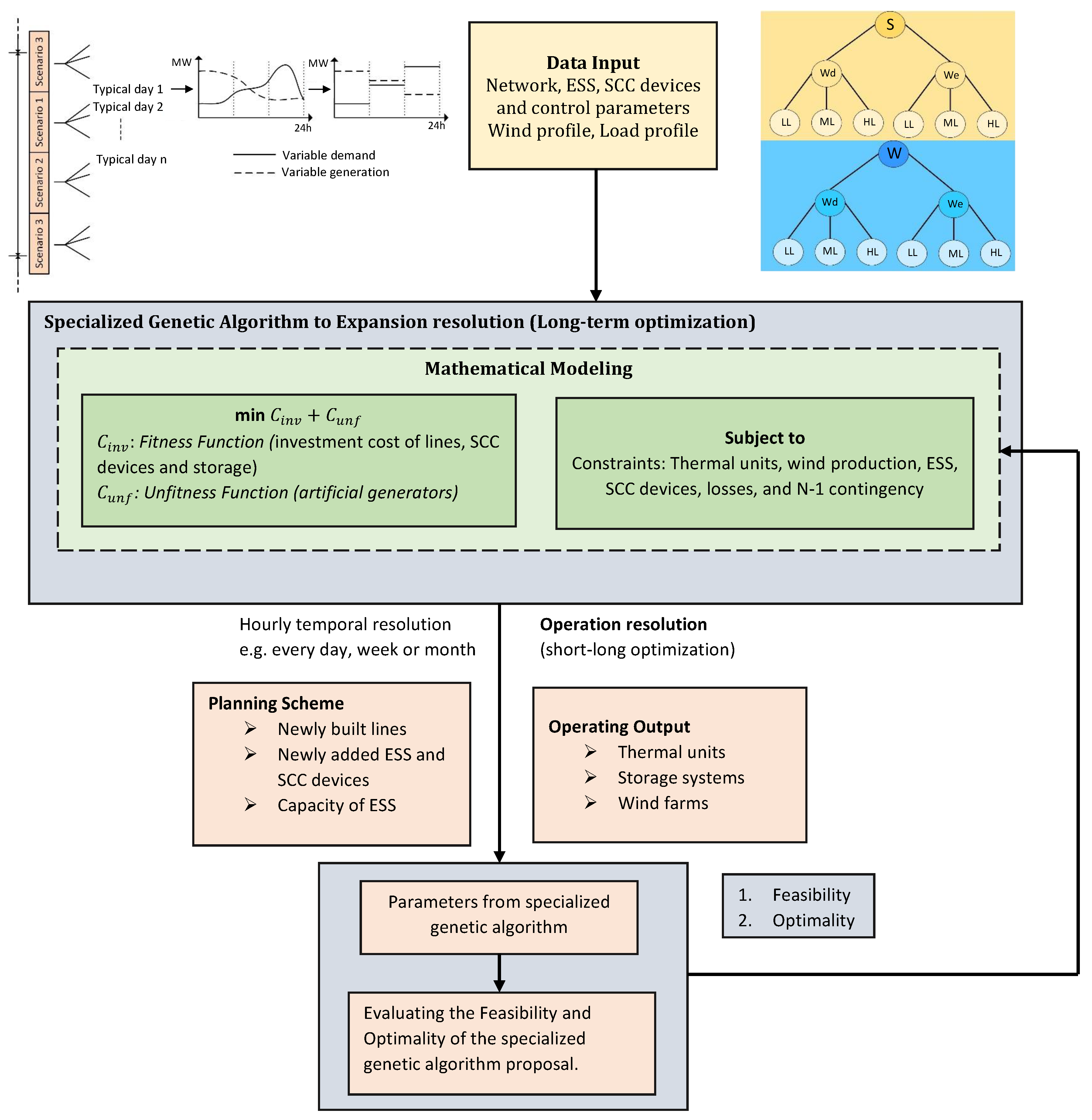
The outline of the planning model in this work addresses a coordinated TEP problem involving intraday time constraints, transmission lines, storage, and series compensation with losses and N-1 contingency. The structure of the proposed methodology is shown in Figure 1, where planning programming seeks to minimize the optimal value of the investment in the newly built facilities. Basically, the specialized genetic algorithm depends on mathematical modeling, marked in green, where the objective function is separated into fitness and unfitness functions. At this stage, the specialized algorithm proposes a configuration or topology for long-term expansion planning, for example, 5 or 10 years (in this paper the 12 scenarios marked in yellow and blue in Figure 1 are used). The specifics of the genetic algorithm are provided in Section 4. In the lower-level optimization marked in orange, the individuals proposed by the algorithm are solved using mathematical modeling again to ensure the viability and optimality of the individuals. In this stage, the configuration proposed by the algorithm for short-term operations planning is evaluated, for example, days, weeks, or months. Note that at this stage, the cost of the unfitness function must be equal to zero.
The scenarios shown in Figure 1 (top) are used to illustrate the variability in load growth and available wind production capacity. Thus, an approach based on energy scenario curves and typical days is proposed for the TEP problem. The stepped demand and wind power curves form the scenarios that will be considered in the formulation of the TEP problem. The higher the level of detail is in this representation, the more accurate the problem modeling will be. However, to maintain the computational effort required for the model solution to be within reasonable limits, it is necessary to limit the number of elements represented (scenarios, typical days, and curve levels). As an illustrative example of this modeling, Figure 1 shows energy scenarios for summer (S), marked in yellow, and winter (W), marked in blue, with attributes such as typical days (weekdays (Wd) and weekends (We)) and load levels (light load (LL), medium load (ML), and heavy load (HL)).
Therefore, the model structure will be represented as in Figure 1, where the TEP problem is modeled with twelve variable generation and demand scenarios. These stepped curves are related to the CBGA, where for each scenario, mathematical modeling is executed to find optimality and feasibility. The step curves are obtained from historical data by applying the arithmetic mean of wind production and daily load.
3. Mathematical Model
In this section, the mathematical model for the TEP problem considering the optimal placement of ESSs and SCC devices with N-1 contingency and power losses is presented [13,15,27,30,34]. The integrated formulation of these concepts is listed below.
where Equation (1) seeks to minimize the total investment cost expressed as the sum of the investment cost in the build of the new line, plus the cost of the installation of the SCC devices involving the number of lines in the base topology , plus the cost of the installation of the ESSs (which are related to the fixed storage cost, variable costs related to charge and discharge power, and unit energy capacity), plus the cost of load shedding. Constraint (2) represents Kirchhoff’s first law, which corresponds to the input/output power of the transmission lines, power losses, thermal plant and wind production, and artificial generators. Constraints (3) and (4) indicate Kirchhoff’s second law, which implicitly imposes nonlinear constraints. Due to these constraints, the TEP problem is formulated as an MINLP problem, where (3) is the constraint without contingency and (4) is the constraint with contingency for each , knowing that is the number of paths. Constraint (5) represents the energy limits for storage in each period and scenario, where denotes the initial storage level starting the day, and is the storage level during , where the charge and discharge efficiency of the storage system in this work are considered unitary. Constraint (6) denotes the storage energy balance per day. The linearized losses computed by adding the linear functions through the piecewise linearization method are expressed through constraints (7)–(11). Note that the model incorporates loss linearization based on [35]. Constraints (12) and (13) represent the power flow limit without and with N-1 contingency. Constraints (14) and (15) are discharging and charging bounds for the ESSs. Constraints (16)–(18) establish the production bounds for thermal plants, wind production, and load shedding. Constraint (19) ensures that the maximum number of lines to be added in branch is not exceeded.
The constraint (20) represents the maximum number of ESSs. Decision variables for storage devices, number of circuits with and without N-1 contingency, and phase angle are represented by constraints (21)–(24). It is worth noting that in this formulation, there are sets of operational variables, with one set designated for each contingency, where all paths are considered .
To obtain the annual equivalent costs, the capital costs of the lines and ESSs in the objective function are converted to annual values by multiplying by the annuity factors [36]
where x is the discount rate, while y denotes the lifespan in years. Although transmission lines and ESSs incur considerable initial costs, their annual costs are relatively lower due to their extended lifespan.
4. Specialized Genetic Algorithm
Genetic algorithms (GAs) are optimization techniques that utilize the principles of natural selection and the evolutionary processes of species. GAs can solve highly complex combinatorial optimization problems with an acceptable computational effort [15,24,37].
In this paper, the Chu and Beasley genetic algorithm (CBGA) proposed in [15] is slightly modified to solve the TEP problem with the optimal placement of ESSs and SCC devices.
To employ the CBGA in the mathematical model of the TEP problem in this work, the objective function is divided into two sub-functions, namely the fitness function (circuits and ESSs costs) and the unfitness function (identifies the unfeasibility of the individual, i.e., the load shedding ).
The characteristics of CBGA are described below.
4.1. Codification
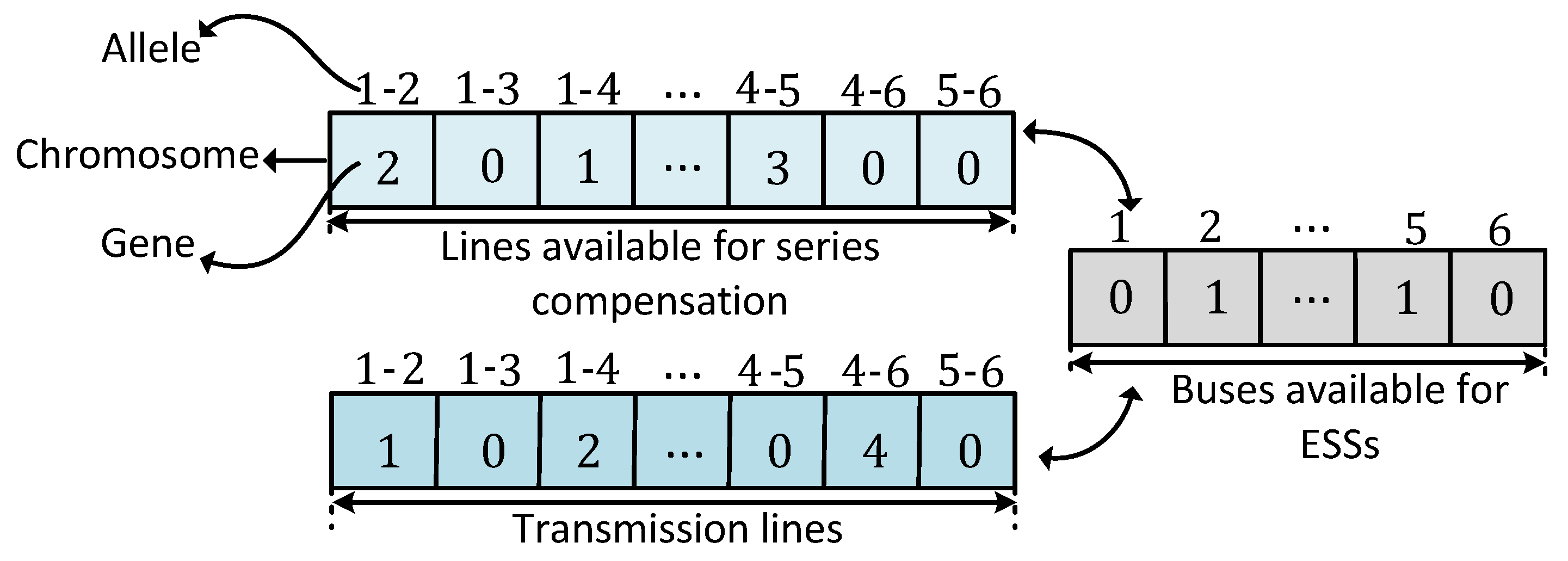
The coding proposal is based on the representation of a candidate solution integrating lines, SCC devices, and ESSs simultaneously. This representation is the most important aspect in structuring the GAs. Coding and integrating equipment may either simplify or complicate the implementation of genetic algorithm mechanisms. Two types of encoding are used in this paper. The first uses decimal coding to represent a proposed solution for lines and SCC devices, and the second uses binary coding to represent a proposed solution of the ESS. The individual is a proposed solution to the problem; that is, it constitutes the topology comprising all the lines, lines with SCC devices, and buses with ESSs added to the corresponding system with an investment proposal. In this work, the CBGA individual is represented by three vectors. The first vector corresponds to transmission lines, the second corresponds to lines with SCC devices, and the third corresponds to buses with ESSs. Each element of this vector is related to a branch of the system under analysis. Figure 2 depicts the coding scheme adopted in this work that is applied to the Garver system, where the complete topology vector, branches , and decision variables are represented as chromosome, allele, and gene, respectively. In Figure 2, branches 1–2, 1–4, and 4–6 have one, two, and four new lines (see line vector) with SCC devices of types 2, 1, and 0 (see line vector available for SCC devices) and with two storage systems, one in bus 2 and another in bus 5 (see vector of storage systems). Note that in each vector, the zero indicates that no element (lines, ESS and/or SCC devices) has been placed. The approach proposed in this work does not require that the coding for buses with ESSs be binary, since it can be represented by a vector that indicates the types of ESSs (similar to the coding of SCC devices) according to their power and energy storage capacity.
4.2. Initial Population
According to the specialized literature, there are two methods to initialize the population of CBGA lines. The first is random and the second uses a constructive heuristic algorithm. For the initial population of the CBGA of this work, the Villasana Garver constructive heuristic algorithm is employed. The initial population for optimal placement of SCC devices is decimal random with serial compensation device types, while for storage systems, it was chosen by a binary random population.
4.3. Selection
There are different selection methods for genetic algorithms, such as roulette selection, tournament, ranking, steady-state, elitism, and Boltzmann selection. In this paper, tournament selection is used. This step consists of randomly selecting individuals from the current population to generate two groups. Once the two groups are generated, they are sent to a competition between individuals. This is performed with the objective of selecting the two best individuals from each group, who will be named parent 1 and parent 2.
4.4. Recombination
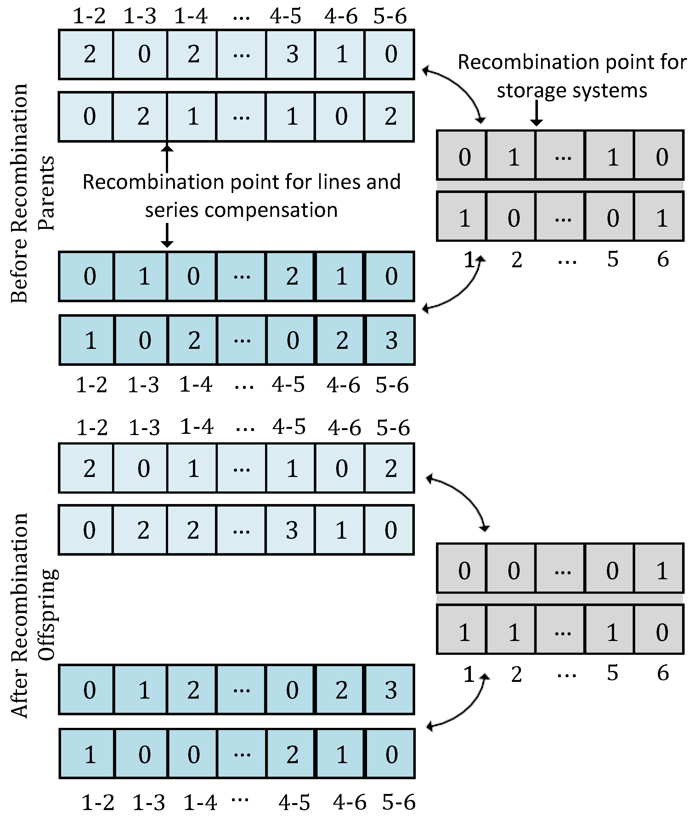
This genetic operator allows the exchange of genes or information between individuals. In this solution, single-point recombination is utilized, wherein a single recombination point is randomly selected, and two offspring are generated for each element. In traditional genetic algorithms, the offspring from all three elements may be incorporated into the population of the succeeding generation. However, in the CBGA, only one individual from each of the elements can be part of the population. Figure 3 shows the recombination for the Garver system. The random point is chosen in corridors 1–3 for lines and SCC devices, whereas for ESSs, the random point is chosen in bus 2. Note that the randomly chosen points for lines and lines with SCC devices are the same. Once the information for the two individuals (parents) has been exchanged, two offspring are generated.
4.5. Mutation
This mechanism of the genetic algorithm allows the current population to have greater diversity and prevents the algorithm from remaining in local minima. Furthermore, the mutation allows the creation of new qualities in the individuals of the current population. Figure 4 shows the mutation process, where branches 1–4 for SCC devices decide to change from type 1 to type 3, while branches 4–5 decide to add a line in the configuration of lines, and for the configuration of ESSs, bus 5 decides to install a storage system. This procedure is contingent upon a mutation rate denoted by , typically falling within the range of 5% to 10% [38].
4.6. Local Improvement of an Individual
A new individual emerges after the processes of selection, recombination, and mutation. This individual may be either feasible or infeasible (non-zero load shedding). Therefore, since the objective function of the CBGA is divided into the unfitness function and a fitness function, local improvement is achieved for both functions, and they are described as follows.
4.6.1. Improving the Unfitness Function
To improve the unfitness function and transform the infeasible individual into feasible (load shedding equal to zero), the constructive heuristic algorithm (CHA) in [39] is used. In this CHA, the capacity limits of the power flows of the circuits are ignored and the DC model presented in [40] is executed to obtain the power flows in each branch. Once the power flows are determined, transmission lines are added to the branch with the highest power flow (overload circuits). This procedure is repeated until there are no more overloaded branches. Completing this process, the individual becomes feasible.
4.6.2. Objective Function Improvement
After using the constructive heuristic making the individual feasible and performing the selection, recombination, and mutation mechanisms, the individual may contain excess elements (lines or storage systems) causing a higher investment cost. Therefore, at this stage, excess elements are eliminated based on the costs of the lines and ESSs without altering the feasibility of the individual.
4.7. Population Substitution
To carry out this process, the procedure introduced in [31] is employed, where the individual that aspires to be part of the current population and replace another individual of the population must follow the acceptance criteria, such as (1) ensuring that the individual differs in features from each member of the current population, where represents the diversity factor. This value is computed using a diversity rate defined in the reference [38], and (2), if the fitness function of the offspring demonstrates superior quality compared to the fitness function of the worst individual in the current population, then the offspring replaces that individual.
4.8. Stop Criteria
In the specialized literature, there are various stopping criteria, such as the number of iterations, when the incumbent does not improve for several generations when the configurations are very similar and when there is practically no diversity of individuals in the populations. Therefore, this paper opts for the number of iterations criterion.
Figure 5 shows the CBGA procedure with SCC and ESS devices. In this flowchart, it is initialized specifying control parameters, such as , , , , , . It is worth mentioning that several studies were carried out on the selection of the levels of each CBGA parameter; thus, it is suggested to start with the following parameters: , , , and ; USD 10, 100, and/or 1000/MW. Here, smaller values represent solving small-sized systems, while larger values represent solving large-sized systems, which are also mentioned in the References [31,38].
5. Test and Critical Analysis of the Results
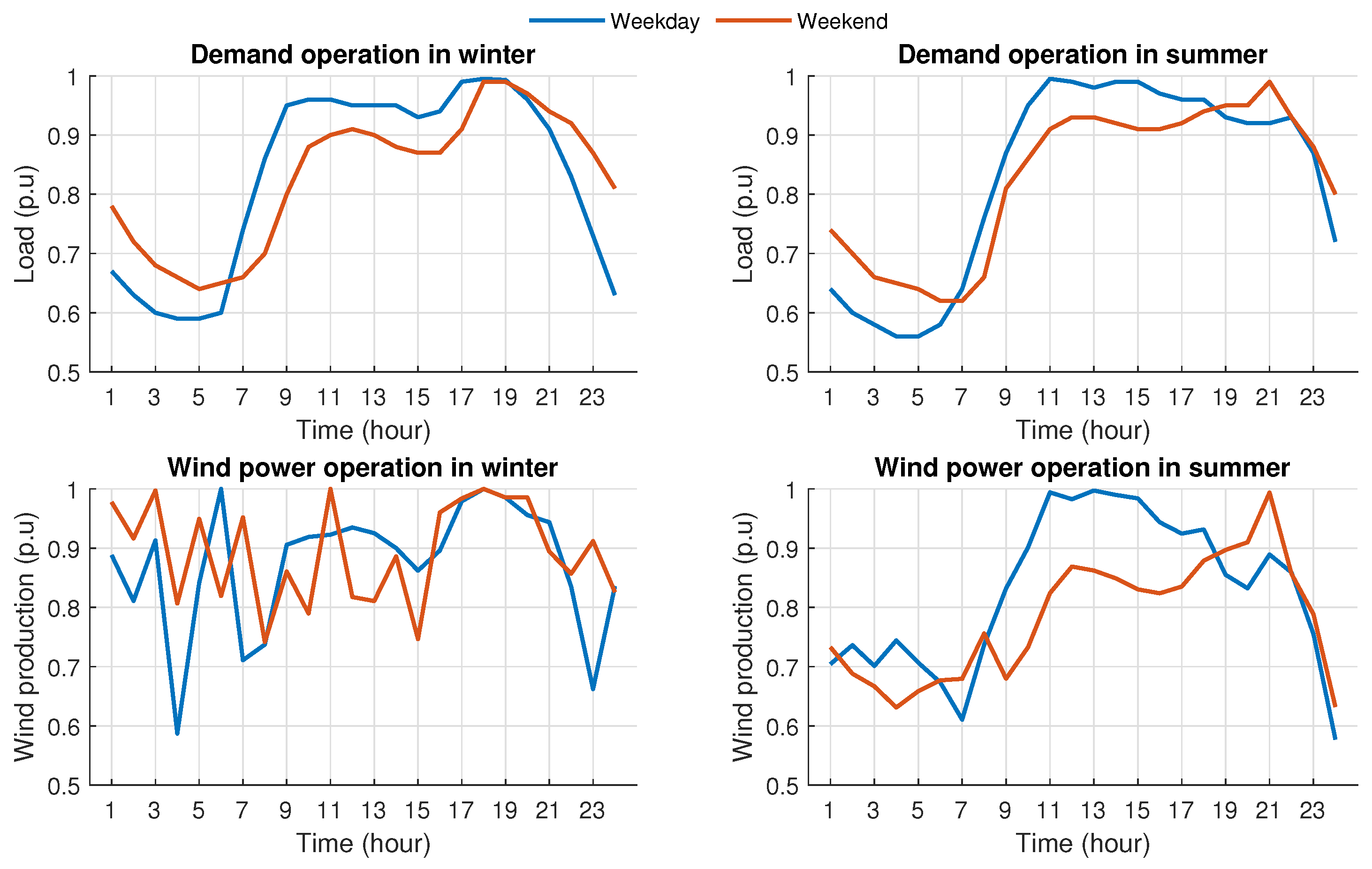
The mathematical formulation presented in Section 3 was developed and successfully applied in Matlab programming language using a personal computer with an Intel processor with 16GB RAM. Garver’s 6-bus test system, the IEEE 24-bus test system, and the modified Colombian system were tested. The electrical data for these systems can be found in [13,15]. All N-1 line-outage contingencies are taken into consideration. The load and wind profiles for winter and summer are shown in Figure 6.
It is assumed that the daily demand is variable according to Figure 6, which establishes 12 demand intervals called scenarios. Table 1 provides the demand coefficients for each scenario. The first six rows correspond to the winter scenario, and the second six rows correspond to the summer scenario. Furthermore, within these scenarios, there are Wd and We classified into LL, HL, and ML. Some nodes with generators installed in the base system will be assumed as wind farms, which will vary according to the following scheme: winter weekdays and weekends (LL-50%, HL-100%, and ML-85%) and summer weekdays and weekends (LL-55%, HL-100%, and ML-80%). It is important to note that this scheme is replicated twice to work with the twelve scenarios in Table 1. Then, using the Weibull distribution, the wind production curve shown in Figure 6 is generated since wind power depends on wind speed.
Table 2 and Table 3 show the data for the installation of ESS and SCC devices, respectively, which are taken from [13,32].
A candidate storage system is taken into account at each node. The fixed cost of each of them is USD 6/kWh to avoid the decisions of ESSs that are too small. In converting the capital costs into annual equivalents, a discount rate of 10% is assumed, and the lifespans of the transmission lines and ESSs are defined as 30 and 15 years, respectively. The variable investment cost parameters, such as the unit cost of power capacity, unit cost of energy capacity, and cycle efficiency, are assumed as follows: 500/KW, 3000/MWh, and [36].
The six cases listed in Table 4 are compared.
5.1. Garver Electrical Test System
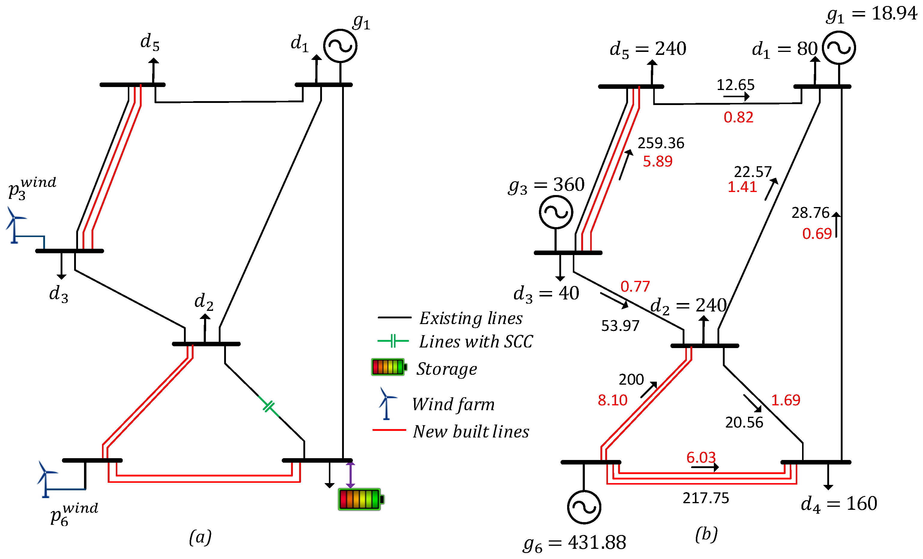
The initial test is conducted on the Garver system, featuring six buses, 15 branches, a load demand of 760 MW, a generating capacity of 1110 MW, and a maximum allowable number of additional circuits per branch set at four. Initially, it has five nodes and six lines connecting them, with the sixth node remaining disconnected from the rest of the system. The base topology and parameters of the existing and candidate lines are referenced in [41]. Two wind farms are placed, one in bus 3 and the other in bus 6, as shown in Figure 7a; each of them varies according to the scheme presented above.
The control parameters of the CBGA for this system in the six cases are: , , , , and .
The planning outcomes for case VI are depicted in Figure 7a. Six new lines are planned, with an installation cost of USD 160.0 million. A storage system is built in bus 4 with fixed and variable installation costs of USD 2.4 and USD 3.66 million, respectively, and a compensated line is added in branches 2–4 type 2, with an installation cost of USD 6.0 million, whereas Figure 7b shows the planning outcomes in case II with seven new lines planned and an installation cost of USD 190.0 million. Values in red indicate power losses.
Figure 8 shows the power flow comparison of three cases for the Garver system. Furthermore, a comparison of the number of lines and power losses for each case is illustrated. It can be observed that when SCC devices are installed, the power losses decrease, but if both the SCC and ESS devices are installed simultaneously, the power losses tend to decrease even more.
The results of all cases are presented in Table 5 with load shedding equal to 0.00 MW. Furthermore, this table shows the construction of new lines to the base topology and investment costs for lines, storage and SCC devices; power losses; the resolved linear programming (LP) numbers; the number of blocks of the piecewise linearization of power losses; and the computational time. Column 8 represents the subtotal cost of transmission lines plus the cost of SCC devices and the fixed cost of storage systems. The cost for case I is equal to the optimal solution reported in [15]. It can be seen that when power losses are considered, the investment cost increases. However, the investment cost tends to decrease when SCC devices and storage are added, even considering losses. For example, comparing case II and case VI, case VI is 9.44% cheaper than case II. Thus, when only SCC devices are added, the investment cost is slightly reduced (see cases III and IV). However, when ESS and SCC devices are installed together in the expansion planning, the investment cost is cheaper (see cases V and VI).
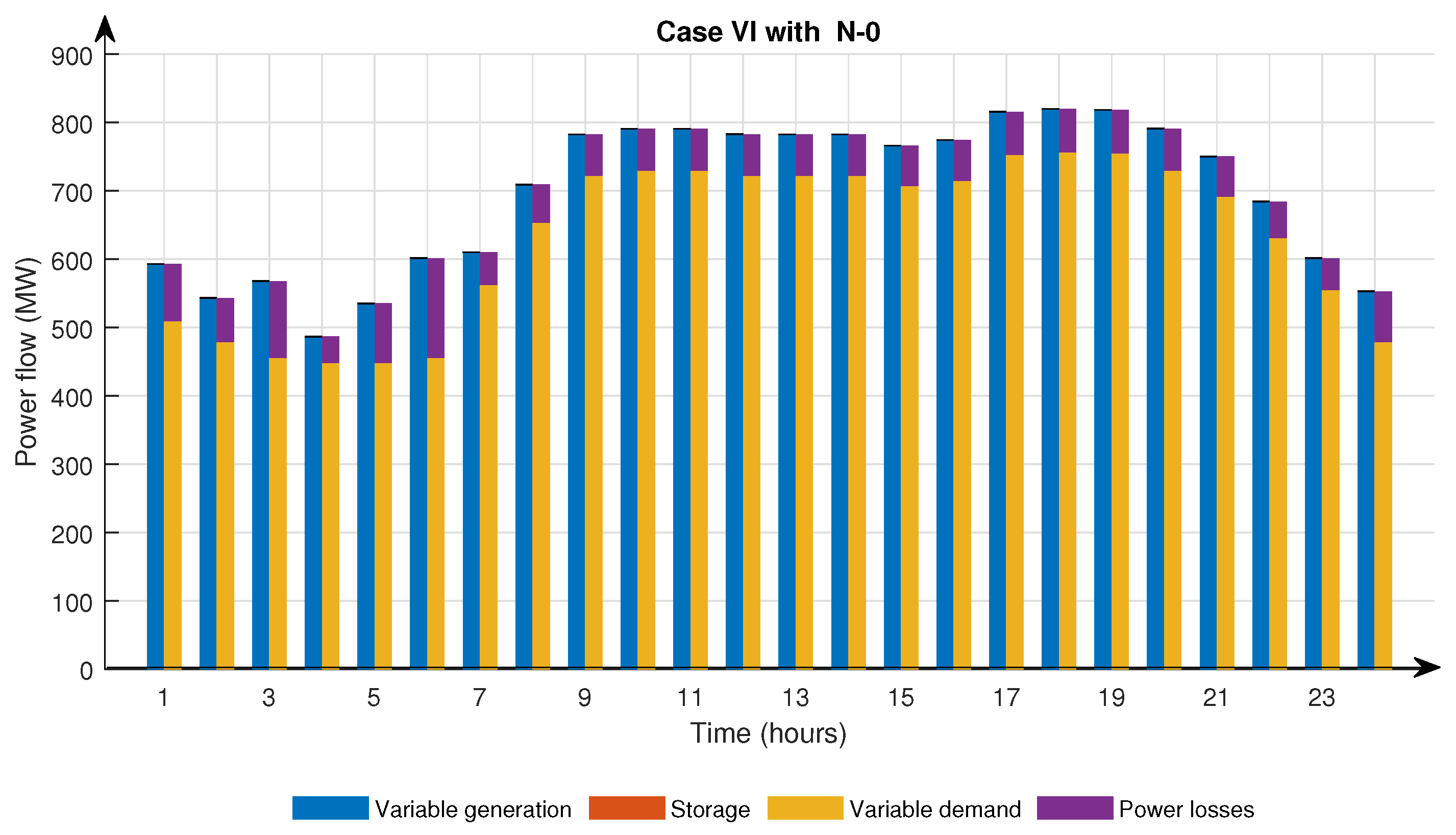
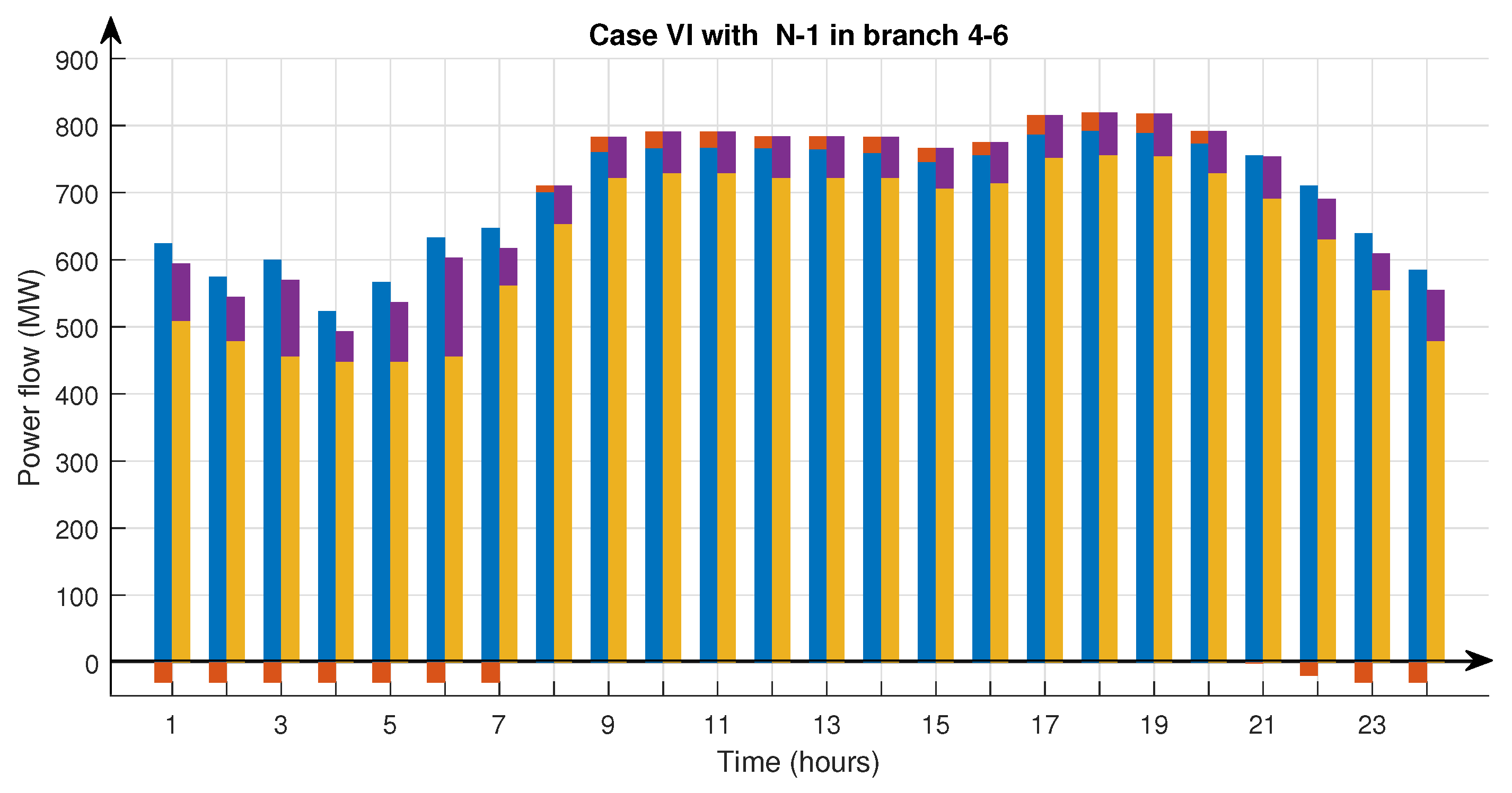
Using the representative daily profile curves shown in Figure 6, Figure 9 illustrates a comparison of case VI with and without storage on a weekday in winter. For case VI, when there is no line outage, that is, N-0, the operation of the system is balanced between generation and variable demand, while when a line is disconnected in branches 4–6, storage is necessary. The findings indicate that the storage system effectively mitigates fluctuations in wind power at nodes 3 and 6. It charges during periods of high wind power output under light load conditions and discharges when wind power output is low during heavy load conditions. It is worth noting in Figure 9 that the power at each hour of the day is the equivalent power of the entire system.
5.2. IEEE 24-Bus Test System
This system has 24 buses and 41 branches and a limit of five circuits that can be added in each branch. The generation capacity is 10,215 MW and the demand is 8550 MW. Two wind farms are placed, one in bus 13 and the other in bus 18. The optimal solutions of the planning problem for cases I, II, V, and VI, using the CBGA control parameters, namely , , , , , and , are listed below, with each test with load shedding equal to 0.00 MW.
Test 1: The optimal solution to the TEP problem in case I is USD 441 million, which is equal to the optimal solution presented in [15]. This optimal solution is found after running 441 LPs with the following topology: , , , , , , , , , and , and with a computational time of 3.67 min.
Test 2: The optimal solution in case II is USD 485 million, with the following base topology , , , , , , , , , , and . This optimal solution is found after running 3556 LPs with a computational time of 36.58 min. The power losses is 177.23 MW with the number of blocks of the piecewise linearization .
Test 3: Taking into account the optimal placement of both ESS and SCC devices in case V, the best solution found has a total investment cost of USD 438.7 million. The investment cost of the lines is USD 419 million with the following topology: , , , , , , , , and and a cost of USD 7.5 million for an SCC device of type 2 installed in and a storage installed in bus 5 with fixed and variable installation cost of USD 5.4 and USD 7.16 million, respectively. This optimal solution is found after running 29,451 LPs with a computational time equal to 83.2 min.
Test 4: Considering power losses for case VI and the optimal placement of the ESS and SCC devices to solve the TEP problem, the best solution found has a total cost of USD 480.72 million. The investment cost of the lines is USD 447 million with the following base topology: , , , , , , , , , and , and investment cost of type 1 and 3 of the SCC devices installed in branches and is equal to USD 16.6 million, and two storage systems are in placement in buses 1 and 2 with fixed and variable installation costs of USD 10.8 and USD 6.32 million, respectively. This optimal solution is found after executing 133,300 LPs with a computational time equal to 21.83 h. The power loss is 209.23 MW with the number of blocks of the piecewise linearization . The solution diagram for this system is illustrated in Figure 10.
Comparing the results only for cases II and VI, the solution obtained in case VI is 0.88% cheaper than case II.
5.3. Practical Application on the Colombian System
The findings detailed in this section are based on a modified Colombian system, consisting of 45 hydroelectric units, four wind farms, 192 transmission lines, and 93 buses. The 14.559 GW loads and 14.559 generation units in the Colombian system are included, together with 12.173 GW from hydro units and 2.386 from wind farms.
The electrical data of this system are found in [13]. In this test system, cases I and V are simulated. To demonstrate the potential benefits of the ESS and SCC devices in transmission expansion planning in the future and to prevent computational burden, power losses were intentionally not considered. The optimal solution of the planning problem for cases I and V and using the CBGA control parameters, namely , , , , and , are listed below, where each system has a load shedding of 0.00 MW.
Test 1: The investment cost necessary to solve the TEP problem considering case I is equal to USD 1185.65 million, with the addition of the following lines to the base topology: , , , , , , , , , , , , , , , , , , , , , , , , , , , , , , , , , , , , , , , , , , , , , , , , , , , , , and ; that is, 65 transmission lines are needed to satisfy the demand. This optimal solution was found after executing 6,662 LPs with a computational time of 24.80 min.
Test 2: Considering case V, the best solution identified by the CBGA considering the optimal placement of the ESS and SCC devices and N-1 contingency has a total investment cost of USD 1063.95 million. The investment cost of the lines is USD 878.79 million with the following topology: , , , , , , , , , , , , , , , , , , , , , , , and and a cost of USD 84.64 million for SCC devices with the following topology: (type 1), (type 3), (type 2), (type 3), (type 2), (type 2), (type 1), (type 2), (type 1), (type 3), (type 3), (type 2), (type 3), (type 3), (type 3), (type 1), (type 2), (type 1), and (type 3) and two storage systems are in placement in buses 45 and 60 with fixed and variable installation costs of USD 72.0 and USD 29.16 million, respectively. This solution was found after solving 494,631 LPs with a computational time of 11.70 h.
The scheme of case V is shown in Figure 11. The generators at nodes , and 81 are wind farms. According to the optimization results, ESSs have been deployed at nodes 45 and 60.
Comparing the results of cases I and V obtained for the Colombian system, in case V it is only necessary to add 31 lines to satisfy the demand. Therefore, it presents an investment cost 10.27% cheaper than case I.
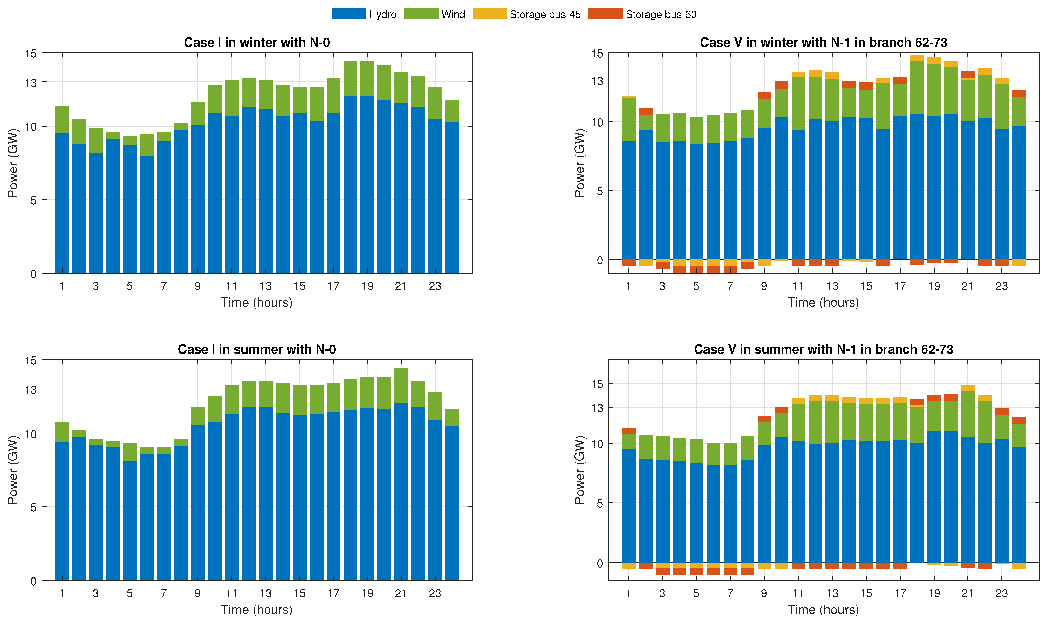
The representative daily curves of wind variation and load demand on the weekend in different seasons are depicted in Figure 6. The power output of different units in cases I and V are contrasted in Figure 12 on a typical winter weekend day. It is obvious that the output of wind energy increases due to charging of ESSs during wind blowing times at light load, and if a line on branches 62–73 is disconnected, the output of hydro units decreases due to the discharging of the ESS during wind weakling time.
Table 6 shows the comparison of annual costs for the three test systems. It can be seen that the annual cost gradually tends to decrease when adding storage and SCC devices simultaneously. In some cases, the construction of new lines decreases. When comparing case I and case V for the Colombian system, the number of built lines decreases from 65 to 31.
Table 7 shows a comparison of the time and cost of installation in new transmission lines for the traditional TEP problem without contingency. The TEP problem can be converted into a mixed-integer linear programming (MILP) problem and can be efficiently solved using a commercial solver. However, according to Table 7, the TEP problem formulated as an MINLP problem and solved using the CBGA is more efficient than the TEP problem formulated as an MILP problem.
On the other hand, to perform a sensitivity analysis, Table 8 shows different solutions for the IEEE 24-bus system for case VI under different discount rates and lifespans of the technologies. Thus, the proportional increase in total annual cost is observed; that is, if the lifespan of the technologies increases, the discount rate will also increase.
According to the results presented in this work, it is suggested that, in practice, batteries be used as energy storage systems with investment costs closer to reality. Likewise, batteries currently present problems related to high maintenance requirements and high investment costs. However, it is expected that future technological advances will allow batteries to be integrated more frequently into transmission networks.
6. Conclusions
This work presents a methodology for TEP that integrates the optimal positioning of transmission lines, storage facilities, and SCC devices in power systems with a portion of wind power. Several scenarios are employed to depict the long-term uncertainty, and the daily charging and discharging cycles of storage systems and their interactions with wind farms are shown under intraday time constraints. The mathematical model of expansion planning is solved using a specialized genetic algorithm that considers both storage and serial compensation.
In addition, transmission expansion planning considering losses and contingencies is a more complex problem because when withdrawing a line in the configuration proposed by the CBGA, the load shedding for each type of operation must be evaluated. Therefore, it presents not only a higher investment cost but also a high computational time. However, it should be noted that expansion planning with losses and contingencies constitutes a more accurate, robust, and real representation of the network functioning, resulting in different expansion plans than those obtained when losses and contingencies are neglected. Although the investment cost of planning with power losses and contingencies is higher, the results show that the installation of SCC and storage in all cases allows for delaying the building of some lines and consequently reduce the investment cost by saving of 15.78%, 7.84%, and 25.88% for the newly built transmission lines to the Garver system, the IEEE-24 system, and the Colombian system, respectively. This is an important aspect since the building of new lines takes a long time. Furthermore, considering the energy scenarios of winter and summer in light, heavy, and medium loads, the injection of the charging and discharging power of the storage could be observed when the TEP problem considers SCC devices, power losses, and contingencies.
Author Contributions
Conceptualization of this study, methodology, software, data curation, investigation, and writing—original draft preparation were contributed by D.H.H.; supervision, visualization, project administration, writing (editing) were contributed by D.M.F.; funding acquisition, resources, writing—review and editing were contributed by M.E.C.B. All authors have read and agreed to the published version of the manuscript.
Funding
This research was supported in part by Coordenação de Aperfeiçoamento de Pessoal de Nível Superior (CAPES) under Grant 001, Conselho Nacional de Desenvolvimento Científico (CNPq) under the grants 04068/2020-0, Fundação de Amparo à Pesquisa do Estado de Minas Gerais (FAPEMIG) under the grant APG-03609-17, and Instituto Nacional de Energia Elétrica (INERGE).
Data Availability Statement
The original contributions presented in the study are included in the article, further inquiries can be directed to the corresponding author.
Conflicts of Interest
The authors declare no conflicts of interest.
Nomenclature
| Indices are as follows: | |
| ℓ | Piecewise linear functions |
| b | Nodes |
| i | Thermal generators |
| Transmission lines from i to j | |
| Obtained annual equivalent cost of lines and storage systems | |
| Contingencies | |
| q | Storage systems |
| s | Scenarios |
| t | Time periods |
| w | Wind farms |
| Sets of | |
| Candidate lines | |
| All lines with SCC devices | |
| Scenarios | |
| Storage systems | |
| Storage systems placed at node b | |
| Thermal plants placed at node b | |
| Wind farms placed at node b | |
| Artificial generators | |
| Candidate and initial network circuits | |
| Constants | |
| Cost of transmission lines (USD) | |
| Fixed cost of storage system q | |
| Charge and discharge variable cost incurred only at the time of ESS (USD/MW) | |
| Investment cost of unit energy capacity | |
| Conductance of line | |
| Cycle efficiency of the ESSs | |
| Penalty parameter linked to load shedding (USD/MW) | |
| Transmission lines susceptance (p.u.) | |
| Number of existing transmission lines | |
| Maximum capacity of lines in branch | |
| Power output capacity of thermal plant i | |
| Predicted power output of wind plant w during time t of scenario s | |
| Upper and lower power for discharging of | |
| storage system q | |
| Upper and lower power for charging of | |
| storage system q | |
| Capacity of line | |
| Upper and lower bounds of the energy level | |
| of system q | |
| Demand at node b during time t of scenario s | |
| T | Count of time intervals |
| L | Count of blocks in the piecewise linear approximation of power losses |
| Maximum angle difference across a line equal to during time t of scenario s | |
| Maximum number of ESSs in the entire electrical system | |
| Charge and discharge efficiency of storage system q | |
| Diversification rate (%) | |
| Mutation rate (%) | |
| Maximum number of individuals (population size) | |
| Selection rate, defined as the size of the tournament utilized in the selection process | |
| Maximum capacity of iterations | |
| Variables | |
| S | Transposed incidence matrix representing branches/nodes within the power system |
| Power flow output of thermal plant i during time t of scenario s | |
| Power flow output of wind farms w during time t of scenario s | |
| Starting energy level of storage system q | |
| Storage system q power output during time t of scenario s | |
| Charging power flow of storage system q during time of scenario s | |
| Discharging power flow of storage system q during time of scenario s | |
| Power flow with and without contingency p of | |
| line during time t of scenario s | |
| Number of circuits added in the branch | |
| Artificial generator in node i with contingency k during time t of scenario s (MW) | |
| Artificial generators vector with elements corresponding to the artificial generation during time t of scenario s (MW) | |
| Non-negative slack variables used to replace | |
| during time t of scenario s | |
| Voltage angle variable associated with the ℓth number of piecewise linear functions during time t of scenario s | |
| Slope of the ℓth piecewise linear block during time t of scenario s | |
| Counter of iterations | |
| Binary decision variable for storage system q at node i | |
| Phase angle in node i during time t of scenario s with | |
| and without contingency p | |
| Percentage (between 0 and 1) of the cost of installing SCC devices in branch | |
| Percentage (between 0 and 1) of the reactive compensation in branch | |
References
- D Andrade, B. The Power Grid: Smart, Secure, Green and Reliable; Elsevier: Amsterdam, The Netherlands, 2017; pp. 1–327. [Google Scholar]
- Luburic, Z.; Pandžić, H.; Carrión, M. Transmission Expansion Planning Model Considering Battery Energy Storage, TCSC and Lines Using AC OPF. IEEE Access 2020, 8, 203429–203439. [Google Scholar] [CrossRef]
- Sidhu, A.S.; Pollitt, M.G.; Anaya, K.L. A social cost benefit analysis of grid-scale electrical energy storage projects: A case study. Appl. Energy 2018, 212, 881–894. [Google Scholar] [CrossRef]
- Ai, X.; Li, J.; Fang, J.; Yao, W.; Xie, H.; Cai, R.; Wen, J. Multi-time-scale coordinated ramp-rate control for photovoltaic plants and battery energy storage. IET Renew. Power Gener. 2018, 12, 1390–1397. [Google Scholar] [CrossRef]
- Han, X.; Liao, S.; Ai, X.; Yao, W.; Wen, J. Determining the Minimal Power Capacity of Energy Storage to Accommodate Renewable Generation. Energies 2017, 10, 468. [Google Scholar] [CrossRef]
- Das, C.K.; Bass, O.; Kothapalli, G.; Mahmoud, T.S.; Habibi, D. Optimal placement of distributed energy storage systems in distribution networks using artificial bee colony algorithm. Appl. Energy 2018, 232, 212–228. [Google Scholar] [CrossRef]
- Liu, J.; Wen, J.; Yao, W.; Long, Y. Solution to short-term frequency response of wind farms by using energy storage systems. IET Renew. Power Gener. 2016, 10, 669–678. [Google Scholar] [CrossRef]
- Li, J.; Ma, Y.; Mu, G.; Feng, X.; Yan, G.; Guo, G.; Zhang, T. Optimal Configuration of Energy Storage System Coordinating Wind Turbine to Participate Power System Primary Frequency Regulation. Energies 2018, 11, 1396. [Google Scholar] [CrossRef]
- Milano, F. Power System Modelling and Scripting; Springer Science & Business Media: Berlin, Germany, 2010. [Google Scholar]
- Shafik, M.B.; Chen, H.; Rashed, G.I.; El-Sehiemy, R.A. Adaptive multi objective parallel seeker optimization algorithm for incorporating TCSC devices into optimal power flow framework. IEEE Access 2019, 7, 36934–36947. [Google Scholar] [CrossRef]
- Zamora-Cárdenas, A.; Fuerte-Esquivel, C.R. Multi-parameter trajectory sensitivity approach for location of series-connected controllers to enhance power system transient stability. Electr. Power Syst. Res. 2010, 80, 1096–1103. [Google Scholar] [CrossRef]
- Leonidaki, E.; Manos, G.; Hatziargyriou, N. An effective method to locate series compensation for voltage stability enhancement. Electr. Power Syst. Res. 2005, 74, 73–81. [Google Scholar] [CrossRef]
- Gallego, L.A.; Garcés, L.P.; Contreras, J. Optimal Placement of Series Capacitive Compensation in Transmission Network Expansion Planning. J. Control Autom. Electr. Syst. 2020, 31, 165–176. [Google Scholar] [CrossRef]
- Rahmani, M.; Vinasco, G.; Rider, M.J.; Romero, R.; Pardalos, P.M. Multistage Transmission Expansion Planning Considering Fixed Series Compensation Allocation. IEEE Trans. Power Syst. 2013, 28, 3795–3805. [Google Scholar] [CrossRef]
- Silva, I.d.J.; Rider, M.; Romero, R.; Garcia, A.; Murari, C. Transmission network expansion planning with security constraints. IEE Proc. Gener. Transm. Distrib. 2005, 152, 828–836. [Google Scholar] [CrossRef]
- Sum-Im, T.; Taylor, G.; Irving, M.; Song, Y. Differential evolution algorithm for static and multistage transmission expansion planning. IET Gener. Transm. Distrib. 2009, 3, 365–384. [Google Scholar] [CrossRef]
- Mahdavi, M.; Sabillon Antunez, C.; Ajalli, M.; Romero, R. Transmission Expansion Planning: Literature Review and Classification. IEEE Syst. J. 2019, 13, 3129–3140. [Google Scholar] [CrossRef]
- Naderi, E.; Pourakbari-Kasmaei, M.; Lehtonen, M. Transmission expansion planning integrated with wind farms: A review, comparative study, and a novel profound search approach. Int. J. Electr. Power Energy Syst. 2020, 115, 105460. [Google Scholar] [CrossRef]
- Neumann, F.; Hagenmeyer, V.; Brown, T. Assessments of linear power flow and transmission loss approximations in coordinated capacity expansion problems. Appl. Energy 2022, 314, 118859. [Google Scholar] [CrossRef]
- Ploussard, Q.; Olmos, L.; Ramos, A. A search space reduction method for transmission expansion planning using an iterative refinement of the DC load flow model. IEEE Trans. Power Syst. 2019, 35, 152–162. [Google Scholar] [CrossRef]
- Abdi, H.; Moradi, M.; Lumbreras, S. Metaheuristics and transmission expansion planning: A comparative case study. Energies 2021, 14, 3618. [Google Scholar] [CrossRef]
- Mahdavi, M.; Kheirkhah, A.R.; Macedo, L.H.; Romero, R. A Genetic Algorithm for Transmission Network Expansion Planning Considering Line Maintenance. In Proceedings of the 2020 IEEE Congress on Evolutionary Computation (CEC), Virtual, 19–24 July 2020; pp. 1–6. [Google Scholar]
- Leeprechanon, N.; Limsakul, P.; Pothiya, S. Optimal transmission expansion planning using ant colony optimization. J. Sustain. Energy Environ. 2010, 1, 71–76. [Google Scholar]
- Romero, R.; Rider, M.J.; Silva, I.d.J. A Metaheuristic to Solve the Transmission Expansion Planning. IEEE Trans. Power Syst. 2007, 22, 2289–2291. [Google Scholar] [CrossRef]
- Keokhoungning, T.; Premrudeepreechacharn, S.; Wongsinlatam, W.; Namvong, A.; Remsungnen, T.; Mueanrit, N.; Sorn-in, K.; Kravenkit, S.; Siritaratiwat, A.; Srichan, C.; et al. Transmission Network Expansion Planning with High-Penetration Solar Energy Using Particle Swarm Optimization in Lao PDR toward 2030. Energies 2022, 15, 8359. [Google Scholar] [CrossRef]
- Gan, W.; Ai, X.; Fang, J.; Yan, M.; Yao, W.; Zuo, W.; Wen, J. Security constrained co-planning of transmission expansion and energy storage. Appl. Energy 2019, 239, 383–394. [Google Scholar] [CrossRef]
- Conejo, A.J.; Cheng, Y.; Zhang, N.; Kang, C. Long-term coordination of transmission and storage to integrate wind power. CSEE J. Power Energy Syst. 2017, 3, 36–43. [Google Scholar] [CrossRef]
- Xie, Y.; Xu, Y. Transmission Expansion Planning Considering Wind Power and Load Uncertainties. Energies 2022, 15, 7140. [Google Scholar] [CrossRef]
- de Paula, A.N.; de Oliveira, E.J.; de Oliveira, L.W.; Honório, L.M. Robust static transmission expansion planning considering contingency and wind power generation. J. Control Autom. Electr. Syst. 2020, 31, 461–470. [Google Scholar] [CrossRef]
- Gbadamosi, S.L.; Nwulu, N.I. A comparative analysis of generation and transmission expansion planning models for power loss minimization. Sustain. Energy Grids Netw. 2021, 26, 100456. [Google Scholar] [CrossRef]
- Huanca, D.H.; Gallego, L.A.; López-Lezama, J.M. Transmission Network Expansion Planning Considering Optimal Allocation of Series Capacitive Compensation and Active Power Losses. Appl. Sci. 2022, 12, 388. [Google Scholar] [CrossRef]
- Aguado, J.; de la Torre, S.; Triviño, A. Battery energy storage systems in transmission network expansion planning. Electr. Power Syst. Res. 2017, 145, 63–72. [Google Scholar] [CrossRef]
- Hu, Z.; Zhang, F.; Li, B. Transmission expansion planning considering the deployment of energy storage systems. In Proceedings of the 2012 IEEE Power and Energy Society General Meeting, San Diego, CA, USA, 22–26 July 2012; pp. 1–6. [Google Scholar]
- Torres, S.P.; Castro, C.A.; Rider, M.J. Transmission expansion planning by using DC and AC models and particle swarm optimization. In Swarm Intelligence for Electric and Electronic Engineering; IGI Global: Hershey, PA, USA, 2013; pp. 260–284. [Google Scholar]
- Alguacil, N.; Motto, A.L.; Conejo, A.J. Transmission expansion planning: A mixed-integer LP approach. IEEE Trans. Power Syst. 2003, 18, 1070–1077. [Google Scholar] [CrossRef]
- Zhang, F.; Hu, Z.; Song, Y. Mixed-integer linear model for transmission expansion planning with line losses and energy storage systems. IET Gener. Transm. Distrib. 2013, 7, 919–928. [Google Scholar] [CrossRef]
- Garces, L.; Romero, R. Specialized Genetic Algorithm for Transmission Network Expansion Planning Considering Reliability. In Proceedings of the 2009 15th International Conference on Intelligent System Applications to Power Systems, Curitiba, Brazil, 8–12 November 2009; pp. 1–6. [Google Scholar]
- Gallego, L.; Garcés, L.; Rahmani, M.; Romero, R. High-Performance Hybrid Algorithm to Solve Transmission Network Expansion Planning. IET Gener. Transm. Distrib. 2016, 11, 1111–1118. [Google Scholar] [CrossRef]
- Villasana, R.; Garver, L.; Salon, S. Transmission network planning using linear programming. IEEE Trans. Power Appar. Syst. 1985, 2, 349–356. [Google Scholar] [CrossRef]
- Ruben, R.; Monticelli, A.; Garcia, V.; Haffner, S. Test systems and mathematical models for transmission network expansion planning. IEE Proc. Gener. Transm. Distrib. 2002, 149, 27–36. [Google Scholar]
- De La Torre, S.; Conejo, A.J.; Contreras, J. Transmission expansion planning in electricity markets. IEEE Trans. Power Syst. 2008, 23, 238–248. [Google Scholar] [CrossRef]
- Conejo, A.; Baringo, L.; Kazempour, J.; Siddiqui, A. Investment in Electricity Generation and Transmission; Springer: Berlin, Germany, 2016. [Google Scholar]
Figure 1.
Structure of the planning formulation.

Figure 2.
Proposed codification.

Figure 3.
Single-point recombination.

Figure 4.
Mutation process.

Figure 5.
Flowchart of the CBGA with storage and SCC devices.
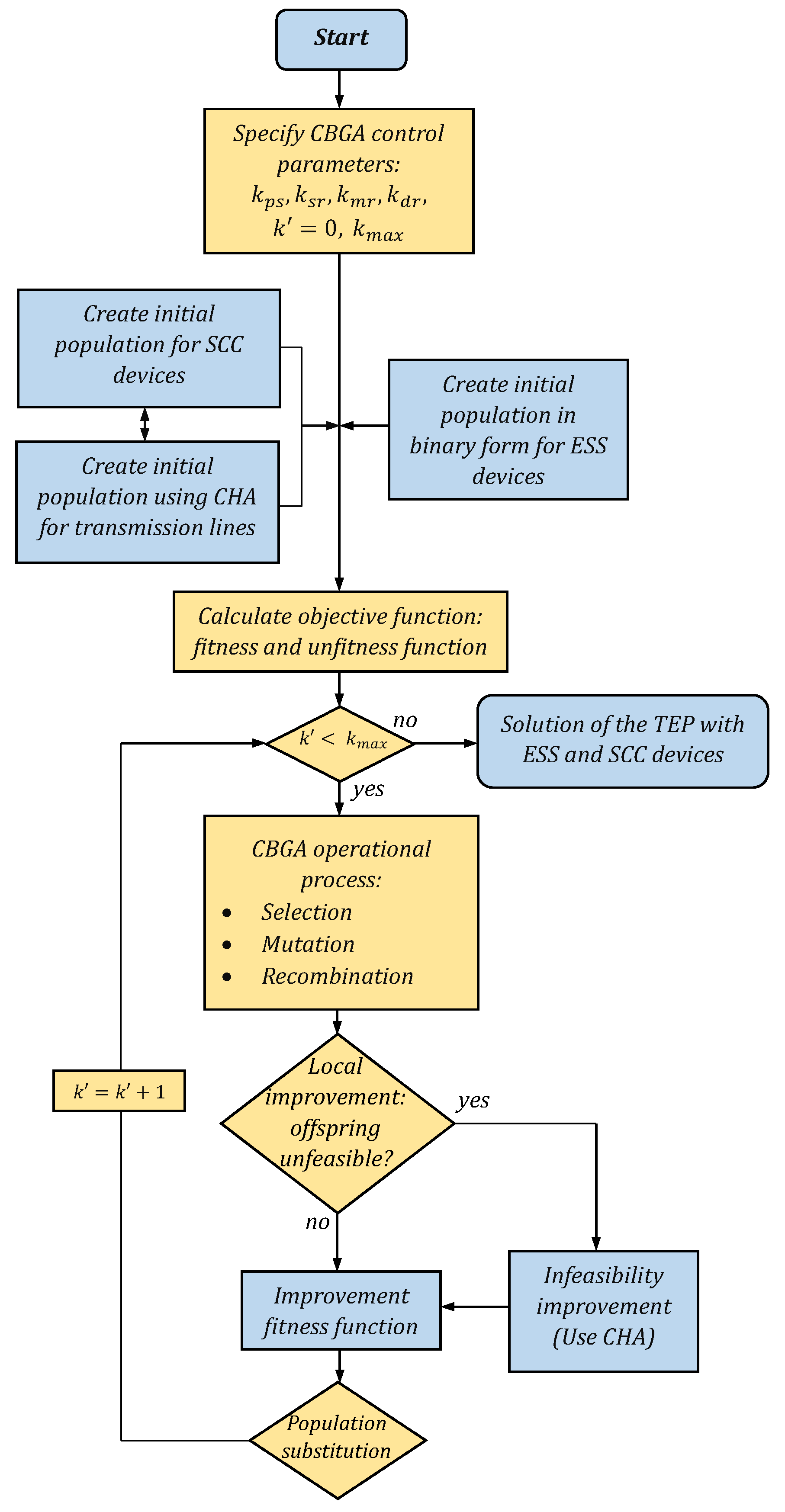
Figure 6.
Representative daily demand profiles.

Figure 7.
Result comparison for two cases: (a) planning outcomes for case VI, (b) planning outcomes for case II.
Figure 7.
Result comparison for two cases: (a) planning outcomes for case VI, (b) planning outcomes for case II.

Figure 8.
Results for three cases.
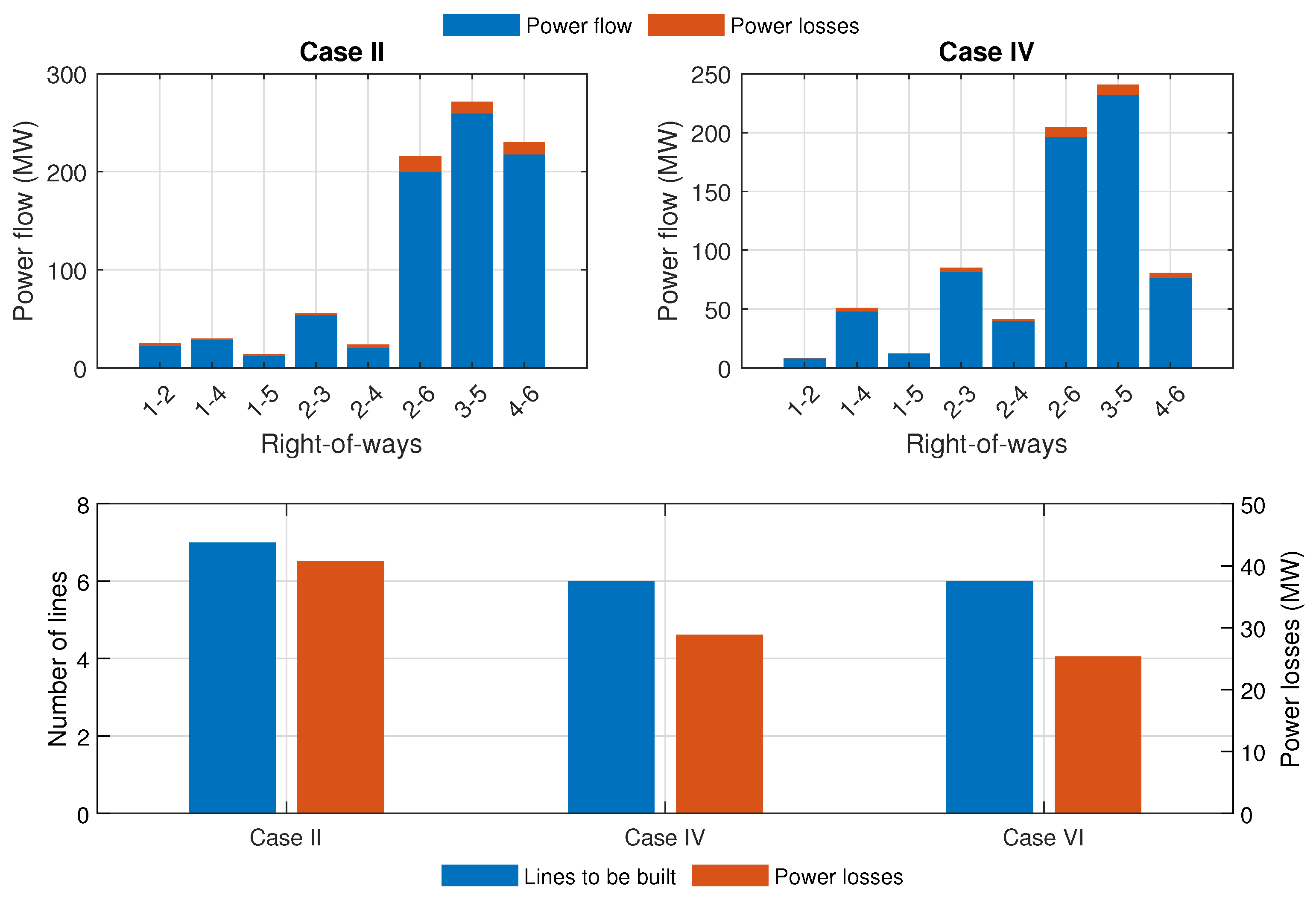
Figure 9.
Energy balance between variable generation and variable demand in the Garver system.


Figure 10.
Optimal TEP solution considering case VI for the IEEE-24 system.

Figure 11.
The case V scheme in Colombian system.
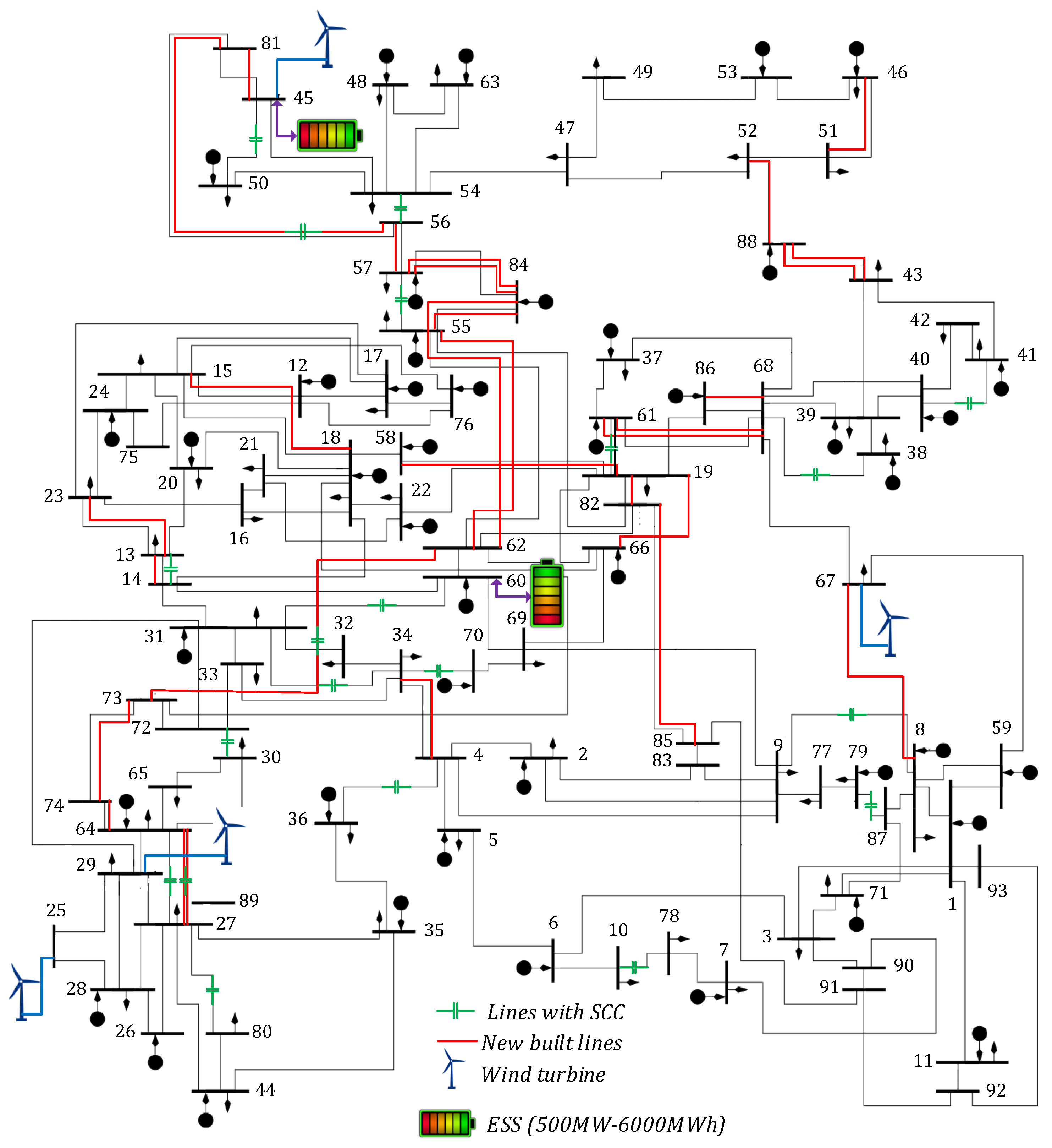
Figure 12.
Power output of units in Colombian system.

Table 1.
Characteristics of each scenario.
| Seasons | Day | Scenario | Demand Coefficient (%) | Load Description |
|---|---|---|---|---|
| Winter | Wd | 1 | 66 | LL |
| 2 | 97 | HL | ||
| 3 | 83 | ML | ||
| We | 4 | 67 | LL | |
| 5 | 97 | HL | ||
| 6 | 82 | ML | ||
| Summer | Wd | 7 | 61 | LL |
| 8 | 98 | HL | ||
| 9 | 80 | ML | ||
| We | 10 | 69 | LL | |
| 11 | 96 | HL | ||
| 12 | 85 | ML |
Table 2.
Storage device characteristics.
| System | (MW) | (MW) | (MWh) | (MWh) |
|---|---|---|---|---|
| Garver | 30 | 0 | 10 | 400 |
| IEEE-24 | 60 | 0 | 20 | 900 |
| Colombian | 500 | 0 | 70 | 6000 |
Table 3.
SCC device types.
| Type | Compensation Rate (Line Reactance) | Compensation Cost (Lines Cost) |
|---|---|---|
| 1 | 0.30 | 0.10 |
| 2 | 0.40 | 0.15 |
| 3 | 0.50 | 0.20 |
Table 4.
Cases to compare the results.
| Case No. | Description |
|---|---|
| Case I | TEP with contingency |
| Case II | TEP considering contingency and power losses |
| Case III | TEP with contingency and SCC devices |
| Case IV | TEP with contingency, SCC devices, and power losses |
| Case V | TEP considering contingency, SCC devices, and storage |
| Case VI | TEP with contingency, SCC devices, storage, and power losses |
Table 5.
Results for the solution of different cases of the Garver system.
| Cases | New Lines | Line SCC (Type) | ESS Node (MW) | Million USD | Losses (MW) | LPs | L | Time (min) | ||||
|---|---|---|---|---|---|---|---|---|---|---|---|---|
| Lines | SCC | ESS | Subtotal | Total | ||||||||
| I | , , , | - | - | 180 | - | - | 180 | - | - | 152 | - | 0.065 |
| II | , , | - | - | 190 | - | - | 190 | - | 40.8 | 715 | 10 | 0.559 |
| III | , , | - | 160 | 8 | - | 168 | 168 | - | 1617 | - | 0.726 | |
| IV | , , | , , | - | 160 | 29.50 | - | 189.5 | 189.5 | 28.87 | 2867 | 20 | 2.830 |
| V | , , , | , | 1(30), 5(30) | 130 | 11 | 10.12 | 145.8 | 151.12 | - | 1625 | - | 0.862 |
| VI | , , | 4(30) | 160 | 6 | 6.06 | 168.4 | 172.06 | 25.32 | 2100 | 10 | 1.731 | |
Table 6.
Annual cost results for the three test systems.
| Description | Cases | |||||
|---|---|---|---|---|---|---|
| Garver | IEEE-24 | Colombian | ||||
| II | VI | II | VI | I | V | |
| Number of new lines | 7 | 6 | 13 | 13 | 65 | 31 |
| Number of added ESS | - | 1 | - | 2 | - | 2 |
| Annual line and lines with SCC devices M USD | 20.15 | 17.60 | 51.46 | 49.18 | 125.77 | 102.19 |
| Annual ESS cost M USD | - | 0.79 | - | 2.25 | - | 13.29 |
| Total annual investment, M USD | 20.15 | 18.39 | 51.44 | 51.43 | 125.77 | 115.48 |
Table 7.
Comparison of cost and time to solve traditional TEP problem without contingency.
| System | Using CBGA This Paper | Using Commercial [42] Solvers (Cplex-GAMS) | ||
|---|---|---|---|---|
| Cost (M USD) | Time (min) | Cost (M USD) | Time (min) | |
| Garver | 110.0 | 0.016 | 110.0 | 0.001 |
| IEEE-24 | 152.0 | 0.020 | 190.0 | 0.073 |
| Colombian | 560.42 | 1.55 | 996.63 | 30.56 |
Table 8.
Solutions for IEEE 24-bus system under different x and y in case VI.
| Discount Rate (%) | Lifespan (Years) | Annual Cost | |
|---|---|---|---|
| Lines with SCC | Storage | ||
| 10 | 30 | 15 | 51.43 |
| 15 | 30 | 15 | 73.53 |
| 20 | 40 | 20 | 96.28 |
| 25 | 40 | 20 | 120.23 |
Disclaimer/Publisher’s Note: The statements, opinions and data contained in all publications are solely those of the individual author(s) and contributor(s) and not of MDPI and/or the editor(s). MDPI and/or the editor(s) disclaim responsibility for any injury to people or property resulting from any ideas, methods, instructions or products referred to in the content. |
© 2024 by the authors. Licensee MDPI, Basel, Switzerland. This article is an open access article distributed under the terms and conditions of the Creative Commons Attribution (CC BY) license (https://creativecommons.org/licenses/by/4.0/).
Share and Cite
MDPI and ACS Style
Huanca, D.H.; Falcão, D.M.; Bento, M.E.C. Transmission Expansion Planning Considering Storage, Flexible AC Transmission System, Losses, and Contingencies to Integrate Wind Power. Energies 2024, 17, 1777. https://doi.org/10.3390/en17071777
AMA Style
Huanca DH, Falcão DM, Bento MEC. Transmission Expansion Planning Considering Storage, Flexible AC Transmission System, Losses, and Contingencies to Integrate Wind Power. Energies. 2024; 17(7):1777. https://doi.org/10.3390/en17071777
Chicago/Turabian StyleHuanca, Dany H., Djalma M. Falcão, and Murilo E. C. Bento. 2024. "Transmission Expansion Planning Considering Storage, Flexible AC Transmission System, Losses, and Contingencies to Integrate Wind Power" Energies 17, no. 7: 1777. https://doi.org/10.3390/en17071777
Note that from the first issue of 2016, this journal uses article numbers instead of page numbers. See further details here.